1. Introduction
Digital transformation and the internet of things (IoT) have led to an increase in interconnected devices used in a variety of different industrial fields. These devices, typically individual sensors acquiring time-encoded data, provide vast potential for automated and data-driven analysis methods from the field of machine learning and deep learning [
1]. The temporal component of the data is essential to identify different patterns and to draw conclusions from the data by finding anomalies, classifying different behavior, or predicting the future temporal course of the time series, and, thus, categorizing the field of time series analytics into three primary tasks: classification, anomaly detection, and forecasting.
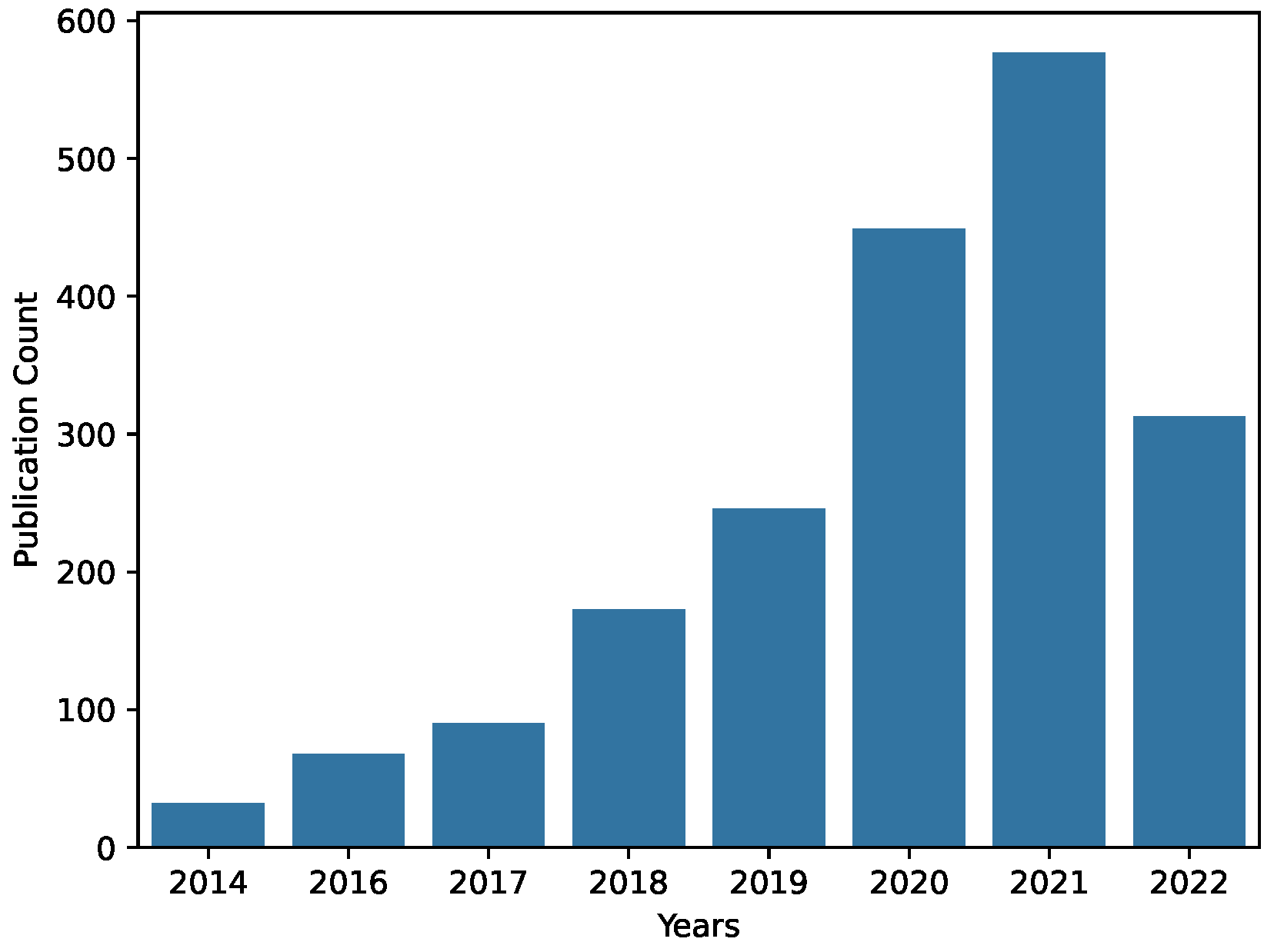
In this paper, we exclusively focused on one of the three main tasks, the forecasting task, which is an increasingly prominent task to be tackled with deep learning models, as shown in
Figure 1. Forecasting is an exciting and relevant problem that combines the need to understand the information in a time series with predicting the most likely future given that information. Moreover, forecasting plays an essential role in supporting the process of decision-making or managing resources [
2].
Despite the high relevance of research on deep learning applications for time series data, the field has not seen a revolution similar to those of computer vision (CV) and natural language processing (NLP). While deep learning has shown remarkable results in learning complex tasks in CV and NLP, traditional machine learning and specialized stochastic models are still perfectly viable and even outperform deep learning models in time series tasks in some cases [
3]. However, such models have disadvantages, including the fact that their creation requires in-depth domain knowledge and their usage often results in high computational costs [
3].
Figure 1.
Illustration of the number of publications per year in the context of time series forecasting and deep learning, extracted on 22 June, 2022, on “Web of Science” [
4] using the query described in
Section 3.
Figure 1.
Illustration of the number of publications per year in the context of time series forecasting and deep learning, extracted on 22 June, 2022, on “Web of Science” [
4] using the query described in
Section 3.
Unlike in the field of time series analysis, the fields of CV and NLP have a number of different benchmark datasets that are frequently used to develop new models and compare cutting-edge developments with prior state-of-the-art models. Therefore, it is common practice for these advancements to be evaluated against these benchmark datasets. Two of the most prominent and widely-used datasets in CV are the MNIST [
5] and ImageNet [
6] datasets for training small and large models, respectively. Specifically, the ImageNet dataset has been frequently used to pre-train large state-of-the-art models that are used for transfer learning, utilizing the pre-trained features for new tasks and individual datasets. Exploiting the pre-trained features allows researchers to achieve state-of-the-art performances even on small datasets after fine-tuning the pre-trained networks. Consequentially, benchmark datasets played an essential role in the advancements of these fields.
Unfortunately, such commonly used benchmark datasets do not exist for all time series tasks, while the frequently used ones are challenged with respect to their data quality. For example, for the common task of time series classification, the UCR/UEA [
7] archive provides a number of datasets, but they contain anomalies and discrepancies that can bias classification results [
8]. Similarly, in the case of the common task of anomaly detection, commonly used datasets exist [
9,
10]. However, Wu and Keogh [
11] showed that these datasets suffer from fundamental flaws. Finally, the task of time series forecasting does not benefit whatsoever from frequently used datasets, let alone benchmark datasets.
The lack of such benchmark datasets for time series analysis is likely due to the unbound character of this particular data type. Images, for example, are naturally bound by the RGB space and the size of the image, i.e., a finite amount of pixels, whereby each one is defined by three values in the closed interval of . Time series are not as well characterized, and values can be, in principal, unbound in the range of . However, practical applications and the laws of physics somewhat limit the range in which time series data is typically acquired. In turn, the vast variety of domains and sensor sources for time series data makes the ranges highly variable. Additionally, the temporal character of the data adds another layer of complexity as time series data are acquired across a large range of temporal resolutions, ranging from nanoseconds to days, months, and years. These circumstances make the development of a cross-domain and cross-task benchmark dataset for time series data highly challenging and the development has yet to emerge until this day.
As a consequence of this lack of a widely recognized benchmark dataset, existing work mainly focuses on comparing different models or within a specific domain on individual domain datasets, as we show in
Section 2. Consequently, this paper aimed to provide a comprehensive overview of the current state of the art regarding openly available datasets for time series forecasting tasks and to address their effect on the research field of deep learning for time series forecasting. The contributions of this work are fourfold:
- 1.
We provide a cross-domain overview of existing publicly available time series forecasting datasets that have been used in research.
- 2.
Furthermore, we analyze these datasets regarding their domain and provide file and data structure, as well as general statistical characteristics, and compare them quantitatively with each other by computing their similarity.
- 3.
We provide an overview of all public time series forecasting datasets identified in this publication and facilitate easy access with a list of links to all these datasets.
- 4.
Finally, we facilitate comparability in the time series forecasting research area by calculating a grouping of datasets using the aforementioned similarity measures.
2. Related Survey Publications
Before we present the results of our own comprehensive survey, we briefly review related work and surveys connected to the task of time series forecasting. For this purpose, we selected publications that reviewed several papers and analyzed how these publications describe and compare the used datasets.
In order to compare these surveys in more than just qualitative terms, we examined each for the characteristics described below, which are summarized in
Table 1. First, we verified the accessibility by reviewing if a dataset was cited (Column 1,
Table 1) and if any effort had been made to allow easy access through a direct link to the data (Column 2,
Table 1). Furthermore, we investigated if multiple datasets were utilized (Column 3,
Table 1), if these datasets were from different domains (Column 4,
Table 1), and if they were compared to each other in text form or in a table (Column 5,
Table 1). Next, we checked if at least two statistical values from each dataset were presented, including size, the number of dimensions, forecasting window, or time interval, shown in the columns “dataset statistics”. Finally, we checked if the datasets were further analyzed in the last column. This could include a comparison by some distance metrics or identifying some characteristics.
The existing work mainly focuses on deep learning architectures, which were compared by all of the publications in
Table 1. This table shows that only three out of 16 publications used datasets from multiple domains, which shows the highly domain-specific view of these publications. Furthermore, no survey satisfied all points. Especially, the analysis of datasets was not conducted by any publication, and the point of providing easy access to the cited datasets was only met by Mosavi et al. [
20]. To conclude, the surveys from
Table 1 show a deficit of publications investigating and analyzing datasets. Especially, a combination of a cross-domain overview, an analysis of the datasets, and easy accessibility was missing. If some statistical values were presented, they were mostly restricted to the length, a forecast horizon, or a time interval. Notwithstanding, more information is needed to make profound decisions about what datasets to use.
Lara-Benitez et al. [
18] stands out by comparing multiple datasets from different domains. In addition, they list the used datasets, give a short description, and show some sample plots. This is the only publication in
Table 1 that met six out of eight points. However, this publication primarily focused on comparing the model architectures. Their research did not focus on the datasets used. In contrast, this work focuses on the datasets used in time series forecasting research.
3. Methodology
3.1. Paper Screening
The primary objective was to identify all relevant datasets with their domains used in papers published in the context of time series forecasting with deep learning. Focusing on recent research in the field of deep learning ensured that the datasets used were still valid and well-known in the community, as deep learning is relatively new to the field of time series foresting.
This combination resulted in a large number of relevant papers. However, two domains could be excluded because of their specific peculiarities meaning they could be considered fields of their own. One of these domains is COVID-19, which has large amounts of publicly available data. However, world data on COVID-19 is already collected and merged by the COVID-19 Data Repository by the Center for Systems Science and Engineering (CSSE) at Johns Hopkins University. The other domain is the field of finance and stock market data which is widely recognized as a field of its own due to its global economic meaning. We excluded this domain due to its extensive amount of publicly available data given by the permanently active stock market and corresponding survey literature [
28].
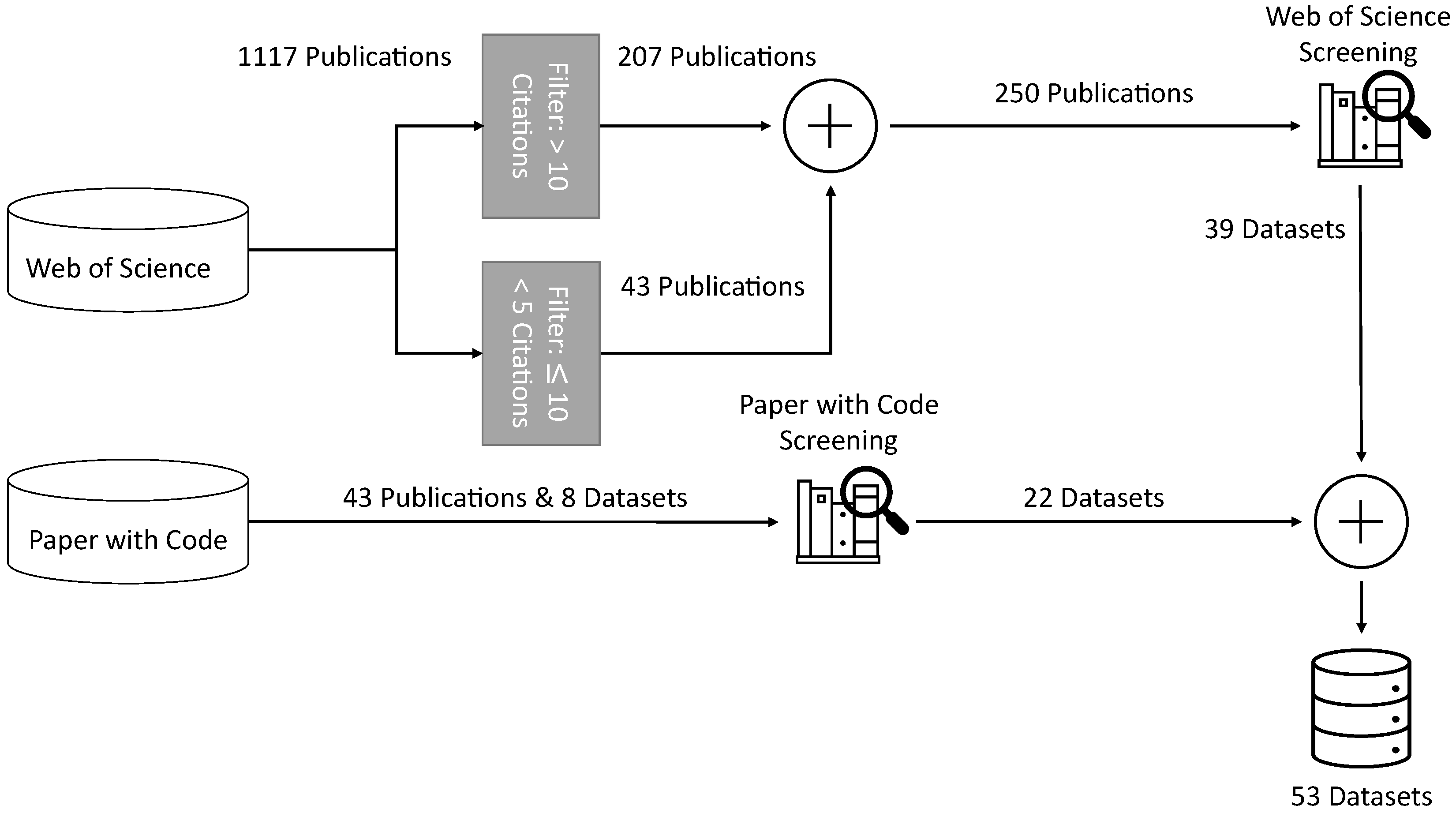
The methodology used in this work consists of three steps and is depicted in
Figure 2:
- 1.
As a first step, we performed a screening of papers found in the “Web of Science” [
4] to identify publicly available time series forecasting datasets which are used in research. To ensure the impact of the datasets in research, we limited our choice to papers that had been cited at least ten times. This reduced the number of papers from over 1000 to 207 and ensured that relevant papers with common datasets were not excluded. Another goal was to identify datasets already used for deep learning. We achieved this by adding the constraint of “deep learning” to the search query. As a result, the following Web of Science query was used:
We focused on examining publicly available datasets and identifying the domains of the selected papers.
- 2.
To address the fact that newly published papers had not had the chance yo acquire ten citations to date, papers from the last year, 2021, had a restriction of having at least five citations and a maximum of ten citations as other papers were already included by step one. Therefore, we used the same Web of Science query as before and extracted 43 new publications on 17 December 2021.
- 3.
To widen the search for datasets used in academic publications, we further utilized the website “papers with code” [
29]. Then, “papers with code” was used to ensure the inclusion of recent publications from conferences that were not listed on “Web of Science”. The “papers with code” website has a collection of publicly available datasets with the associated papers that have published their code and results on a dataset. Furthermore, the website ranks publications per dataset by the number of stars of their corresponding Github repositories. We filtered the datasets by the categories of “time series” and “forecasting” to collect the datasets with their corresponding publications. We selected the top 10 ranked publications if a dataset had more than ten publications, resulting in 43 additional publications with eight datasets. Then, we used these publications for additional screening of datasets to find public datasets not identified by the website “papers with code”.
After combining the before-mentioned steps, we utilized 293 publications. Based on these publications, we identified 53 different public datasets. Moreover, we identified 39 datasets while screening the papers from “Web of Science” and 22 datasets with the website “papers with code”. Eight of the 22 datasets overlap with the datasets from the website “papers with code”.
3.2. Fundamentals of Statistical Time Series Characteristics
In this section, we briefly introduce three statistical measurements that we utilized to identify stationarity, seasonality, and whether a time series dataset consists of repeating values.
Identifying if a time series is stationary shows if the statistical properties change over time and that there is no trend or shift in the time series. This impacts the methods used to analyze the datasets or forecast values from the dataset. Moreover, it shows that the mean, variance, and covariance are constant and independent of time. Consequently, we decided to use the augmented Dickey–Filler (ADF) test [
30].
The ADF test is a widely used unit–root test, which is an extended version of the Dickey–Fuller test. It is derived from an autoregressive (AR(
k)) model and shows if a time series is stationary [
31]. The ADF test removes the structural effects from the Dickey–Fuller test and involves the following regression:
with
,
as the difference operator,
being white noise, and
representing the null hypothesis of the unit root test [
32]. A
p-value lower than 0.05 confirms the null hypothesis and indicates that a time series is stationary [
33].
Most tests for seasonality need domain knowledge, a graphical analysis, or certain assumptions [
34]. Therefore, we decided to use auto-correlation (AC) to identify to what degree a time series correlated with itself or a lagged version of itself. The resulting value indicated if a time series had many repeating patterns, which indicates seasonality. Moreover, the resulting value
with
is the aggregated mean with a maximum lag
of 40 and the sequence length
n [
35].
Furthermore, we computed the percentage of reoccurring values (PRV) to show to what percentage a dataset consisted of repeating values. The PRV values show the percentage of how many values are not unique in a time series. This metric has the disadvantage that it depends on the dataset size because the probability of repeating values grows with the size.
4. Time Series Domains
The high variability in research and application domains of time series analysis makes analyzing domains challenging. For example, suppose two groups of authors of two different papers came out related to a different field of research. In that case, two papers might refer to the same domain but use different wording because of specializations and domain expertise. For example, one can refer to the domain wind speed forecasting as “power load forecasting for renewable energy sources”. In this case, the goal is to forecast the energy output. First, however, the wind speed or other energy-generating factors are forecast to achieve that goal.
To ensure a wide cross-domain overview, we used the publications identified in “Web of Science”to analyze domains according to the following rules. If a paper referred to multiple datasets, the domain of every dataset was counted. On the condition that a domain occurred less than three times, we checked whether the domain could be subsumed in a different domain. If not, the domain was not visualized in
Figure 3 but listed in
Table 2. On the contrary, if one domain occurred more than 30 times and the domain could clearly be separated into different sub-domains, they were divided into these sub-domains. For example, the weather domain could have included the domain wind speed. However, even without the publications of the wind speed domain, the weather domain had more than 30 publications. As a result, the wind speed domain was excluded and treated as a separate domain.
Figure 3 presents the different domains and their frequency in the reviewed literature. The largest domain is the electricity domain. This domain includes publications that forecast the energy output of renewable energy sources, other energy sources, and the consumption of small groups or single households. The second-largest domain is the weather domain. This domain includes multiple weather forecasting publications that highly overlap with publications of the electricity domain’s renewable energy sources. Furthermore, the wind domain could be seen as a sub-domain of the weather domain. Nevertheless, many papers forecast wind speed without considering other weather-related measurements. Correspondingly, we separated the wind speed domain, the third most often screened domain. Next, the air quality domain includes publications that mostly forecast the air quality of cities. Some work published in this context used weather-related features to improve their forecasts. Therefore, the publications show a slight overlap with the weather domain.
Despite the proposed web of science query, which should have ignored the finance domain, the domain was identified as the third most common domain. Nevertheless, as previously set, we ignored publications within this domain entirely. The occurrence of finance publications was caused by publications using more specific keywords than finance.
The high variability in domains indicates that the time series field is mostly domain-driven and time series occur in many different domains, which is shown in
Table 2. Contrary to expectations, some domains did not appear frequently. For example, we expected a high relevance of the machine sensor domain driven through industry 4.0. Nevertheless, machine sensor publications were only seen less than three times. Then again, this phenomenon was likely due to the general aversion of companies to publish their proprietary data in order to protect their intellectual property. Another reason could be that time-encoded machine sensor data is mostly used to classify different states or errors and not directly to forecast.
Furthermore, environmentally-related domains, including weather, wind speed, air quality, and geospatial data, accounted for 35% of all domains. Moreover, the top five domains accounted for around two-thirds of all papers.
5. Screening of Public Datasets
Table 3 and
Table 4 shows a non-domain-specific overview of public time series forecasting datasets collected by the before-described methods. Moreover, the datasets in the tables were selected with the following conditions:
- 1.
Our first condition was that the data must be publicly accessible and not hidden behind a particular sign-in, or only available on request, to give an overview of general publicly available datasets.
- 2.
The dataset must be directly downloadable as files to ensure reproducibility. Datasets that can only be accessed through a web view or dashboard, where multiple parameters need to be selected, were not included.
- 3.
Datasets would not be considered if the data was only available in a specific country or the website was not in English, to ensure consistent access to the datasets.
Datasets with IDs 0 to 38 were found during the paper screening of the 250 identified papers, and all datasets with IDs higher than 38 were found using the website papers with code. The datasets with the IDs 3, 6, 23, 24, 25, 26, 29, and 38 were identified through the “Web of Science” and “papers with code” screening. These datasets are presented in combination with their relevant information on domain, structure, and how the dataset is provided. A direct link to each dataset can be found in
Table 3 by using the ID of the dataset. The missing values in
Table 4 were caused by the different formats in which the datasets were published. If a dataset had multiple files with different formats and dimensions, it was impossible to obtain these values. Furthermore, if an equation or algorithm generated the dataset synthetically, the attributes of the table depended on the generation and were, therefore, not relevant in this context.
We analyzed the data extracted from
Table 4 by investigating the number of citations per dataset to determine if a commonly used benchmark dataset existed. A benchmark dataset is one that should have been cited by a high percentage of the publications found in
Table 4, have a size that can be used for deep learning, and include multiple domains. In addition, we looked for datasets already accepted by the research community.
However, only four datasets were cited multiple times if we only considered the datasets and papers from the “Web of Science” paper screening. Moreover, the maximum number of citations from the “Web of Science” paper screening held the dataset with ID 2 with four citations. In contrast, we observed that the “papers with code” screening resulted in a maximum of 16 citations in one dataset. All datasets from
Table 4 were cited on average
times.
Furthermore, the electricity dataset with ID 16 was the most cited dataset in
Table 4 with 16 citations resulting from the “papers with code” screening, where one paper was already identified through the “Web of Science” screening. The dataset is primarily used for multivariate forecasting. This indicates that the dataset with ID 16 is a common dataset for multivariate forecasting. However, the dataset only covers the electricity domain, and other datasets in the same publications are not as frequently used and vary. Consequently, it was not a benchmark dataset as defined in our work.
On the other hand, the dataset with ID 38 (M4 dataset) was used in a competition and was the second most cited dataset compared to other datasets in this work. Furthermore, the dataset combined multiple domains and consisted of 100,000 randomly sampled time series from the ForeDeCk database [
88]. As a result, we found that the dataset with ID 38 was the closest dataset to a benchmark dataset. Moreover, there already exists a follow-up competition with the M5 dataset [
89], which included the forecasting of 42,840 unit sales of the retail company Walmart. The M4 dataset is not a commonly used dataset, as we identified the M4 dataset only once during our “Web of Science” paper screening, although there were more than ten citations on the “papers with code” website.
Next, we analyzed the number of public datasets in different domains to identify the essential domains for time series forecasting with publicly available data. We found no dominating domain, as no domain appeared more than eight times in the table. Moreover, “weather” was the most common domain, occurring eight times, followed closely by the electricity domain with seven occurrences and the air quality domain with five occurrences. Additionally,
Table 4 shows that domains with public datasets varied and were not restricted to a few domains. Even domains identified less than three times, seen in
Table 2, have public datasets.
Furthermore, we investigated the number of dimensions , data points n with where , and time intervals to investigate if a typical pattern existed. Moreover, the number of dimensions shows that time series data is naturally multivariate. All of the datasets had at least three dimensions, where at least one dimension was temporal. Moreover, the other dimension could include locations, categorical variables, a forecasted value, and variables that present additional information. The number of data points from the datasets varied from to , had an approximate average of , and an approximate median of . Moreover, the size or number of data points of the dataset depended on the time interval. If the time interval was daily or yearly, the dataset was most likely smaller because the data had to be recorded over a much larger time period. The two datasets with an annual time interval had an average number of 10,886 data points, while the average number of data points from the datasets with a one-minute time interval was 1,441,804.
Table 4 shows that the column “Data Structure” varies, as only 57% of the values from the data structure column exclusively had “+” values. Furthermore, the timestamp was missing in 28% of the datasets. This can be problematic if some time features, like holidays or other seasonal effects, are relevant to a forecasting task. Finally, considering the different file formats in which the datasets were published, the CSV format was the most used format with 62%, and the second most used format was the text format, which included data in a table structure similar to the CSV format. As a result, we could conclude that there is currently no established standard way of publishing a time series dataset.
Furthermore, we identified multiple challenges while screening the selected papers for datasets, like non-unique names of datasets from different domains, different parts of a publication where the datasets were described and cited, a false web link, or no link to the dataset. Consequently, it would be helpful for reproducibility to refer directly to the dataset used. Furthermore, the data’s availability could increase the subject’s visibility and the work done. The missing publicly available data could be caused by restrictions made by the data owner if the data came from a company because the company may not want to give their competitors insights. Another reason could be privacy concerns if user data is involved. If an author only wanted to show that deep learning has the potential to improve forecasting in his research field, it would not be his first concern to make the data publicly available. On the other hand, authors who wanted to introduce a new deep learning model should have comparability in mind and use a publicly available dataset or make their datasets publicly available.
Nevertheless, sometimes, publications only describe what the data is and which features are present in the data. Some other papers, for example [
90,
91], describe where they extracted the data and which parameter they used to select their training and testing data. These papers would be reproducible in principle if the data sources were still available. However, in some cases, the linked data source can be unavailable in a particular country or not available anymore in general. Hence, it is impossible to access the data with the original URL. An example is a company or institute with a changed web domain or website structure. Another option to cite a dataset is to cite a publication that introduced the dataset. However, this could also be problematic if the cited paper does not have a direct link to the referred to dataset.
To summarize,
Table 4 shows that there are some large datasets publicly available that are already used in the context of deep learning. Nevertheless, these datasets are widely spread between the different domains. Due to the high percentage of public datasets that come out of domains with less than three publications and many publications only using one dataset from one domain, we concluded that the time series forecasting research field is primarily domain-driven. Additionally, we identified that publishing datasets are not common in time series forecasting and that there are multiple reasons why authors are not publishing their datasets. Finally, we determined that even though some datasets are more frequently used, a commonly used benchmark dataset does not exist.
6. Comparison of Selected Datasets
In this section, we aimed to extract general patterns or statistics of the dataset to identify commonalities and differences between the datasets. We chose to rely exclusively on statistics and distances that could be computed automatically without any manual effort. To give a better overview of the available datasets and the underlying structure of the data, we analyzed datasets by multiple statistical methods. Only a subset from
Table 4 was used because the datasets and their description had to meet the following requirements:
- 1.
The forecast value must be clearly defined in a paper or a dataset description.
- 2.
The defined forecasting value should not be aggregated over a period of time or locations.
- 3.
For comparability, the target must be a univariate time series.
For all further analysis, the determined dimension of the forecasting value was used for comparison with other datasets, which can be found in the “Forecasting Value” column of
Table 6. Even though one dimension does not represent the full datasets and their characteristics, the target dimension is the most important dimension in a forecasting task, and restriction is needed to ensure comparability.
6.1. Comparison of Selected Datasets with MPdist
We decided to use the MPdist measurement to compute the distance from all datasets to each other. The MPdist measurement can be used for different time series lengths and is robust against spikes, dropouts, and wandering baseline [
92]. MPdist shows if two time series share similar subsequences under the euclidean distance [
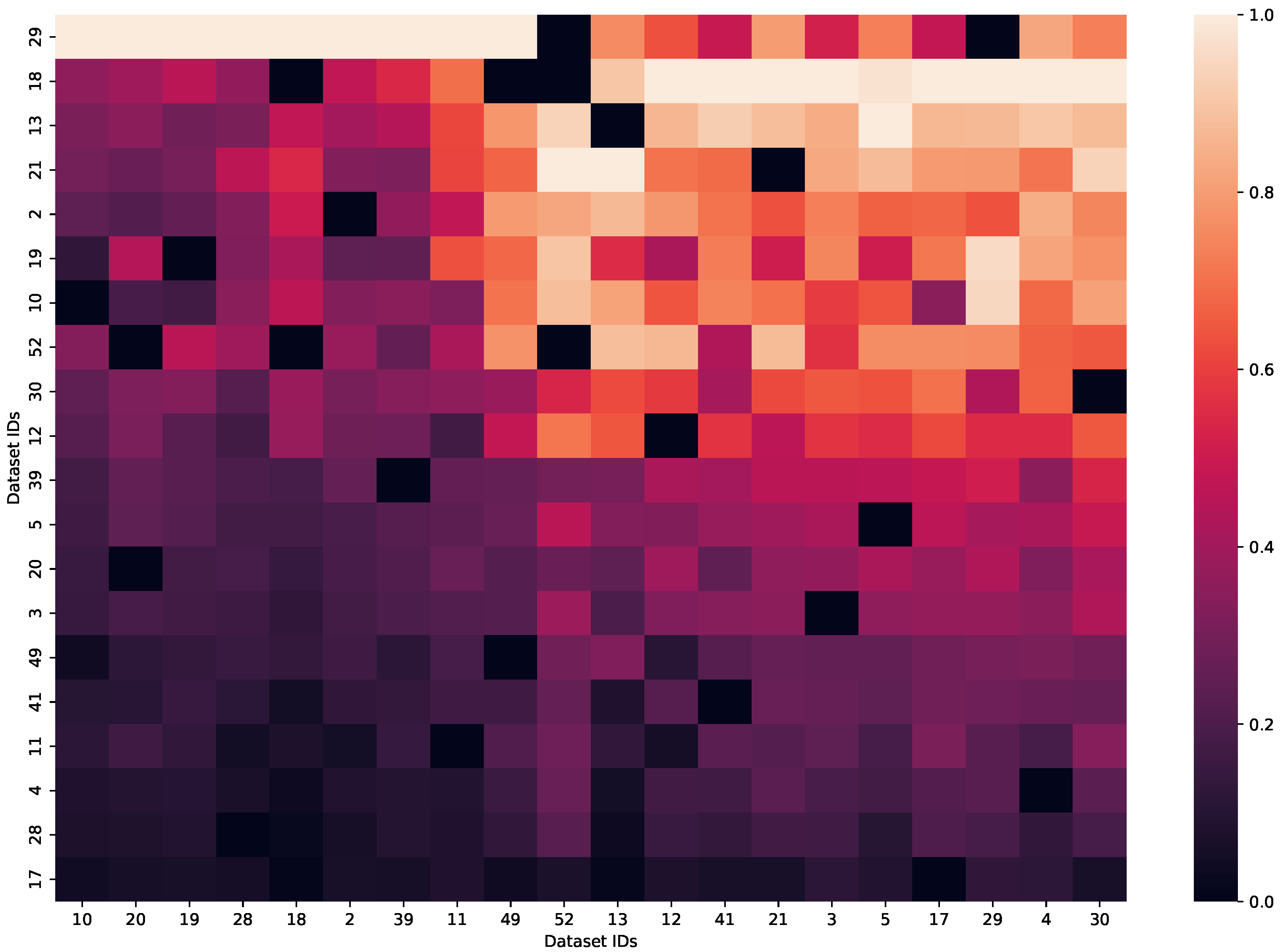
92]. We utilized MPdist to visualize the normalized distance between all datasets in
Figure 4. The distances resulted from first computing the maximum subsequent window using Matrix Profile [
93] and then using the window to compute the MPdist normalized by the window size.
Figure 4 illustrates the sorted distances of the datasets. We sorted the heatmap in both dimensions so that the datasets with the lowest distances were in the bottom left corner, and the highest distances were on the top right side. MPdist is not a symmetrical distance measurement, so it results in different distances depending on the direction of the distance computations. Moreover, if we computed the distances between two datasets
and
, we computed
and
.
Furthermore, the black colors of
Figure 4 show that the datasets were similar under the MPdist, and the light orange colors show that the datasets did not share many subsequences.
Figure 4 shows that datasets 17, 28, and 4 were the datasets with the lowest distance to all other datasets, which is presumably correlated to common patterns in these datasets that can be found in multiple of the other datasets with their corresponding window size. Nevertheless, these datasets were not the ones to which most other datasets were the closest, meaning that despite their common patterns, the other datasets did not have patterns with their corresponding window size that could fit into these datasets.
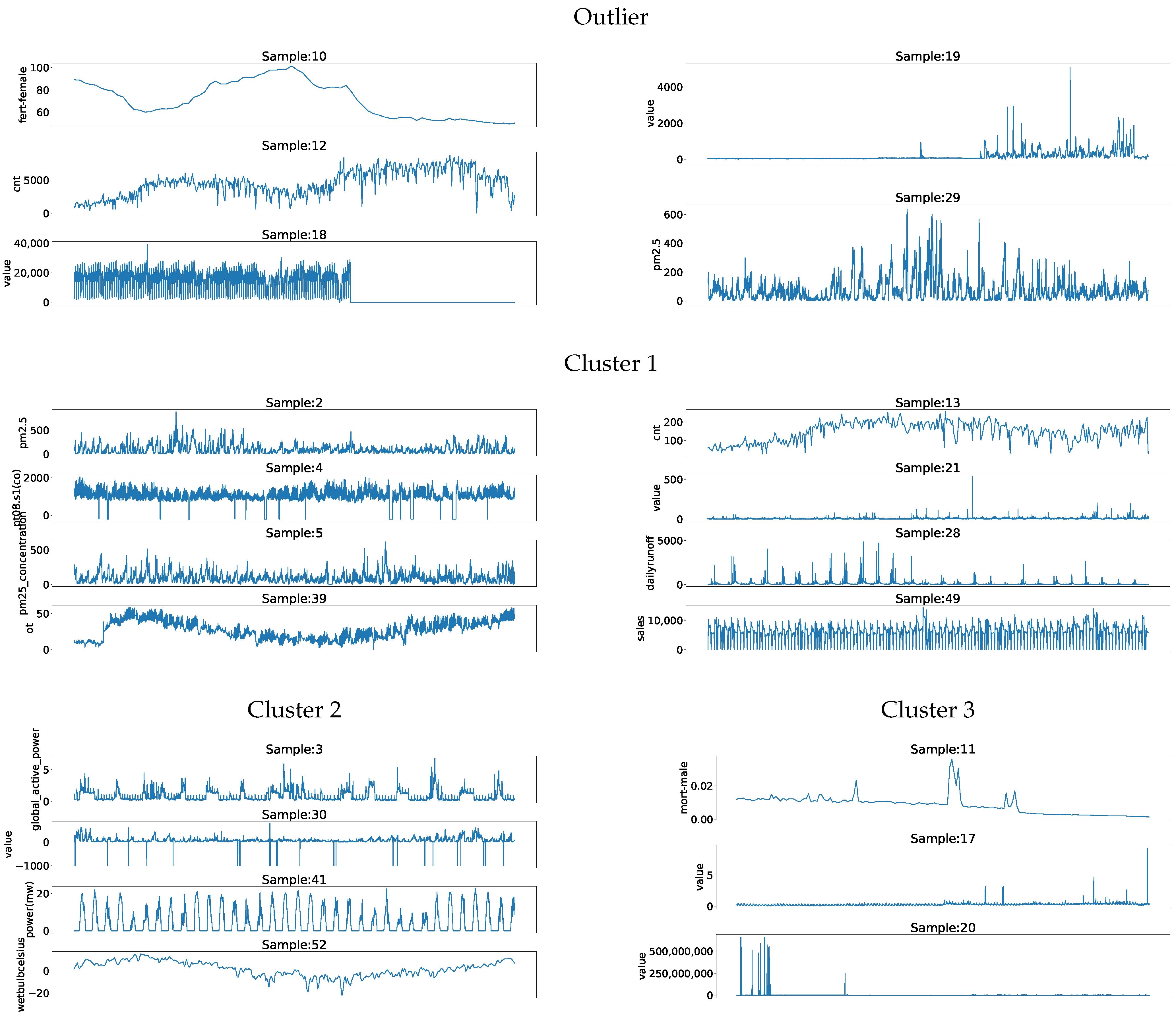
Figure 5 presents samples from all datasets. These samples show that datasets 4, 17, and 28 had frequent short peaks, which could be fitted well into the other datasets.
Datasets 10, 20, and 19 were the datasets to which most other datasets were the closest. This could be caused by patterns of these datasets that are common in other datasets regardless of a certain window size. The dataset with ID 10 was an outlier due to its small size. Moreover, combining the small dataset size with large window sizes of other datasets could lead to some bias in the results and should be carefully considered.
Furthermore, datasets with IDs 18 and 29 had high distances to most other datasets. The dataset with ID 18 contained data from multiple domains, and combined with the one computed window size could lead to high distances. The dataset with the ID 29 had longer irregular peaks, which might not be fitted into different datasets well. Moreover, this dataset was the dataset to which the other datasets had the third highest distance. This indicated that these irregular peaks did not match with the other datasets in both directions.
The MPdist measurement enabled us to compare datasets directly to one another. Nevertheless, we needed more than the distances to draw general insights or to group the datasets. Therefore, we utilized the MPdist distance matrix for clustering in
Section 7 to draw more general insights.
6.2. Comparison of Selected Datasets with Statistical Characteristics
The before-shown MPdist measurements only compare the datasets directly against each other, and, when adding a new dataset, all distances to and from the new dataset must be computed. This makes a fast comparison to new datasets impossible. Therefore, we decided to use additional statistical values to enable other researchers to compare their datasets and find similar datasets without having to rely on extensive computation. Unfortunately, there are no commonly used advanced statistics that are applicable and could describe a complete time series dataset. As a result, we focused on three different statistics representing characteristics like trend, seasonality, and repeating values, which are described in
Section 3.2.
To compute the statistical values ADF, AC, and PRV, the dataset column with the forecasting values was used to calculate the metrics with the ts-fresh library [
94]. If a dataset exceeded the number of 1M data points, a representative contiguous sample of the size with 1M data points was used for the computation.
Table 6 shows that around 90% of the datasets were stationary. Only the datasets with IDs 10, 12, and 18 were not stationary. Furthermore, the datasets with the IDs 10 and 12 were the smallest datasets with less than 1000 data points. Datasets with a low number of data points could include more likely trends if the datasets were not recorded for an extended period. Then again, the dataset with ID 18 was larger and had nearly 70k data points. Next, the auto-correlation values showed a high variance in the datasets. The AC values started at
and went up to
with a mean of
and a standard deviation of
. The AC values were mostly equally distributed, except for a small focus of values near zero. Finally, the PRV showed two distributions with one outlier. One distribution included high PV values over
, and the other included low values under
. Furthermore, the outlier with ID 19 did not lie in these two distributions, with a PRV value of
. This indicated characteristic differences in the studied datasets, which could be grouped or categorized.
7. Categorize the Datasets
As we have discussed, time series forecasting of datasets out of different domains exists. However, there are multiple domains in which only one or no public time series forecasting dataset exists. This makes it difficult to compare model performance as the similarity of the used datasets to train and evaluate these models cannot be investigated. Therefore, we introduced a method to find datasets with similar characteristics to enable researchers to publish comparable results if a used dataset cannot be published due to, for example, privacy concerns or company restrictions. Then, these found datasets can be used in addition to the original dataset to publish results that are reproducible for other researchers.
We identified clusters from the already computed ADF, AC, PRV, and MPdist values. We utilized the density-based DB-scan [
95] clustering algorithm with the hyperparameters
and
, determined by an initial visual-assisted hyperparameter search. Moreover, we used AC, ADF, PRV, and MPdist, weighed equally, as input for the DB-scan algorithm. Using MPdist as an additional distance for the clustering algorithm had the advantage of enforcing similar patterns under the euclidian distance in the later-derived categories.
Table 7 presents an overview of the values from
Table 6, which are divided into four different clusters with corresponding outliers.
The clustering resulted in five outliers which can be seen in the first part of
Table 7. Furthermore, the first cluster was the largest cluster, including eight datasets. Moreover, the second cluster included four datasets, and the third cluster had three datasets. Interestingly, three out of four datasets from the air quality domain could be found in cluster one, suggesting some degree of similarity between these datasets given their domain. However, it was also the largest cluster, and only the combination of weather and bike-sharing and electricity appeared in addition to the air quality domain more than once. Furthermore, the second cluster included the electricity domain twice, and the third cluster consisted only of different domains.
Furthermore, the second cluster’s mean number of data points was the largest, with 1,705,981, followed by the first cluster, with a mean of 528,922 data points. Cluster three had the lowest average data points of 32,850. Both non-stationary datasets could be found in the outliers.
The first cluster had AC values lower than 0.56 and PRV values higher than 0.76. Then, the second cluster had AC values higher than 0.59 and PRV values higher than 0.88. Next, the third cluster had PRV and AC values below 0.1. Based on these clustering results, we defined the ranges of categories. First, we defined high PRV values as higher than 0.75, low values as lower than 0.25, and medium values as within the range of low and high. AC values were high if the value was higher than 0.59 and low to medium if the values were lower than 0.59. We combined low and medium for AC because the clustering suggested that a clear border between the groups did not exist.
Thus, we derived the following categories, which include a grouping of similar characteristics.
- 1.
stationary/high PRV/low to medium AC: This category is a time series that is stationary and has many repeating values which are not distributed in regular patterns or distributed in some regular patterns. Similar datasets could be found in cluster one.
- 2.
stationary/high PRV/high AC: This category is a time series that is stationary and has many repeating values which are distributed in regular patterns. Similar datasets could be found in cluster two.
- 3.
stationary/low PRV/low AC: This category is a time series that is stationary and has many unique values which are distributed in irregular patterns. Similar datasets could be found in cluster three.
- 4.
stationary/low PRV/high AC: This category is a time series that is stationary and has many unique values which are distributed in regular patterns. We only identified the dataset with ID 18 in the outlier cluster. This indicates that this category does not naturally appear in datasets used in research. This could be caused by the multiple domains which are combined in that dataset.
- 5.
non stationary: Due to the small number of datasets we identified which were not stationary, this category could not be used for comparison. It is possible that there were multiple additional clusters that we did not identify. Nevertheless, the work done in this paper could be an indicator that there are not many stationary time series datasets for forecasting used in publications.
8. Conclusions
In this paper, we reviewed publicly available datasets used in publications in the field of time series forecasting using deep learning. We provided a cross-domain overview of the different time series forecasting datasets published in the context of deep learning. Furthermore, we analyzed these datasets regarding their domain, file, and data structure, as well as statistical characteristics and similarity measures, to enable other researchers to choose a dataset on a profound base of knowledge. Additionally, we provided links to all of these datasets to facilitate easy access. Finally, we categorized datasets and provided a method to find similar datasets within a group of similar characteristics, which can be utilized to publish comparable results if the researcher cannot publish their datasets.
The reviewed studies showed that many different time series domains have available public datasets. We did not find a single domain from which most of the public datasets originated. However, a big part of the research is still domain-driven. As a result, publications dealing with time series forecasting use different datasets, leading to a lack of comparability. This may be part of the slowdown in deep learning progress in this area. Even if publications used multiple datasets to test their models, they differed so that there were no commonly used datasets.
To summarize, we identified the research gap of a strongly needed general time series forecasting benchmark dataset, which would improve the progress made in the field of time series forecasting. Furthermore, this analysis shows five categories of datasets. Thus, to construct a representative benchmark dataset, one should consider covering a combination of these categories in a conglomerate of datasets so that all possibilities are included. Likewise, this work can be seen as a first step towards creating a representative cross-domain benchmark dataset for forecasting, focusing on providing an overview of the current state of research. This current state has shown a lack of non-stationary and weakly patterned datasets, which should be included in a benchmark dataset. Therefore, the next steps of creating a benchmark dataset include researching which datasets are used outside scientific publishing and combining multiple datasets from different domains with different characteristics to incorporate a representative cross-domain benchmark dataset. More statistical measurements could extend the method of finding datasets with similar characteristics to cover additional characteristics of time series in future work.


