
Intervention Time Series Analysis and Forecasting of Organ Donor Transplants in the US during the COVID-19 Era

Department of Statistical Sciences and Operations Research, Virginia Commonwealth University, Richmond, VA 23220, USA
*
Author to whom correspondence should be addressed.
Forecasting 2023, 5(1), 229-255; https://doi.org/10.3390/forecast5010013
Submission received: 4 January 2023
/
Revised: 11 February 2023
/
Accepted: 14 February 2023
/
Published: 18 February 2023
Abstract
:The COVID-19 pandemic has had a catastrophic effect on the healthcare system including organ transplants worldwide. The number of living donor transplants performed in the US was affected more significantly by the pandemic with a 22.6% decrease in counts from 2019 to 2020 due to concerns of unnecessarily exposing potential living donors and living donor recipients to possible COVID-19 infection. This paper examines donor transplant counts obtained from the United Network for Organ Sharing from January 2002 to August 2021 using an intervention time series model with March 2020 as the intervention event. Specifically, donor transplant counts are analyzed across the different organs, donor types, and some major individual sociocultural factors, which are potential conditions contributing to disparities in achieving donor transplant equity such as age, ethnicity, and gender. In addition, the kidney allocation policy implemented in March 2021 is introduced as a second intervention event for kidney donor transplants. Overall, forecasts generated by our methods are more accurate than those using seasonal autoregressive integrated moving average models without interventions and seasonal naive methods. The intervention time series model provides a forecast accuracy comparable to the exponential smoothing method.
1. Introduction
More than 107,000 patients in the United States are awaiting organ transplants. Every day, an estimated 33 people in the United States die while waiting for their transplant. For the past four years, on average, only 37,500 organs were transplanted annually, including around 31,000 organs from deceased donors and 6500 organs from living donors [1]. The severe acute respiratory syndrome coronavirus 2 (SARS-CoV-2) that caused the coronavirus disease (COVID-19) pandemic has, among many other things, devastatingly impacted solid organ transplantation (SOT) worldwide, in turn affecting potential donors, candidates, and recipients. While the number of deceased donor transplants remained unaffected, there was an overall decrease of 22.6% from 2019 to 2020 in the number of living donor transplants performed in the US [2]. Ref. [3] noted a strong temporal association between the increase in COVID-19 infections and a striking reduction in overall SOT procedures. Although deceased donation showed an increase of 10.1% and living donor transplants showed a 14.2% increase in 2021 over 2020, their totals were still lower compared to previous years [4]. Due to limited resources and preparedness for the pandemic, the healthcare system, including the organ transplant system, was disrupted. There were some predictive tools and platforms developed as a response to the pandemic. Ref. [5] introduced tools that used a machine learning method to predict the need for hospitalization using a large set of different COVID-19 patient types in southeastern Spain. The CIoTVID IoT platform was presented in [6] to help fight the propagation of the COVID-19 pandemic. To better understand the COVID-19 pandemic’s effect on SOT, it is important to statistically analyze, model, and forecast the profound impact of COVID-19 across various social factors that lead to inequities in donor transplants. The evaluation of the impact of any organ allocation policy that was introduced as an emergency response to the pandemic is also very essential. For example, on 15 March 2021, the organ procurement and transplantation network (OPTN) launched a new policy to match kidney transplant candidates with organs from deceased donors [7]. This kidney allocation policy replaced the 11 OPTN organ allocation regions with a more consistent measure of distance between the donor hospital and the transplant hospital for each candidate and aimed to increase equity in access to transplants. This policy was intended to reduce geographical disparity, pretransplant deaths, and maximize pediatric transplantation. Although the organ allocation system has been subjected to multiple changes with the introduction of new policies over time, our interest lay here in testing the effect of the most recent kidney allocation policy since it brought big changes to the organ allocation system.
Literature on the medical or clinical outcomes of solid organ transplantation is by now vast. However, there are limited studies available specific to analyzing donor transplant counts and forecasting them using a time series analysis in the COVID-era. Ref. [8] examined deceased donor and living donor kidney transplant trends using density mapping and linear regression with an interrupted time series analysis, which is also called intervention time series analysis (ITSA). They found that kidney transplants were affected significantly in recent months due to COVID-19. In [9], adult transplantation data from 1990 to 2019 were analyzed using an autoregressive integrated moving average model (ARIMA) in order to forecast the 2020 expected rates of organ transplants and waitlist registrations. A significant association between the pandemic and the deficit in kidney transplantation and waitlist registration existed. The ARIMA model with interventions could be an efficient method for policymakers to generate forecasts and to evaluate policy interventions or the effect of any major incident affecting donation rates, waitlist registrations, and transplant rates [10]. It is very flexible and easily accounts for seasonality, autocorrelation, underlying trends, and the different types of intervention effects [11,12]. Ref. [13] employed a quarterly interrupted time series regression analysis for estimating the impact of EU regulatory label changes for diclofenac in 2013 among people with cardiovascular disease in Denmark, the Netherlands, England, and Scotland. A review of the interrupted time series analysis in drug utilization research can be found in [14].
In this study, we model the effect of the COVID-19 pandemic as an intervention event on donor transplant time series in the US across different donor types, organs, and select major individual sociocultural factors such as age, ethnicity, and gender, contributing to disparities in achieving donor transplant equity [15]. Research in the past and data over the years have demonstrated that disparities occur at every stage of the transplant process and waitlist registrations with different factors contributing to each [16,17]. Accurate forecasting methods could help public health response with better preparedness and mitigation strategies in events such as the pandemic and any seasonal episodes. Additionally, the kidney allocation policy introduced in March 2021 is modeled as a second intervention event for kidney donor transplants. The forecasts of organ transplant counts from the intervention time series analysis model are then compared with those from the seasonal ARIMA (SARIMA) model without intervention, the exponential smoothing (ETS) method, and the seasonal naive (SNAIVE) method. Studies like ours could help improve the quality and response for maximizing donors in the organ transplant system.
The rest of this paper proceeds as follows. Section 2 introduces the intervention time series analysis model that underlies our work and briefly reviews the ETS and SNAIVE forecasting methods. The forecast accuracy measures used in the study as well as the Diebold–Mariano tests for equality of forecast accuracy are also presented in Section 2. Section 3 summarizes the model estimates and forecasts for various donor transplant time series. Concluding remarks and future works close the article in Section 4.
2. Materials and Methods
2.1. Data Sources
Monthly donor transplant data in the US across donor type, organs, age group were collected from the United Network for Organ Sharing (UNOS) [2,18] for the period from January 2002 to August 2021. For ethnicity and gender, monthly donor transplant data were collected from January 2002 to May 2021. Since the COVID-19 pandemic was declared a national emergency on 13 March 2020, the OPTN approved emergency policy action on 17 March 2020. Thus, all the data prior to March 2020 were considered preintervention with March 2020 being the intervention event for the study. For kidney transplants, the kidney allocation policy was considered as the second intervention event in March 2021.
2.2. Intervention Time Series Analysis
Intervention time series analysis is commonly used to measure the effect of an intervention event on the time series of interest [19]. The time of occurrence of the intervention event is assumed to be known and the intervention can be natural or man-made [20]. In general, the intervention event affects the time series by changing the mean function of the process. In this study, we investigated the effect of the COVID-19 pandemic on organ donor transplantation time series.
The time series model we consider in this section with a single intervention event that occurred at a known time T has the form:
where denotes the intervention effect on time series , and represents the underlying time series without the effect of the intervention event. Here, the effect of the COVID-19 pandemic is described by the model
where B is a backward shift operator, which is defined by . is a pulse function at time T that is used to model an intervention with temporary effect, given by
The model in Equation (2) can be rewritten as
Note that when , it reduces to an MA(1) type filter:
In the case when , it is called an AR(1) type filter:
with a delay of one time-unit before the intervention takes effect. Here, T denotes March 2020 and we assume that the initial condition . Thus, , , and for , , which would represent the transient effect of the COVID-19 pandemic. Specifically, the COVID-19 pandemic caused an immediate change in the organ transplant counts with a magnitude in March 2020 and a strong decreasing effect with a magnitude in April 2020, followed by a gradual decay at the rate back to the original pre-COVID level with no permanent effect. Here, , , and are unknown parameters to be estimated.
With the intervention effect specified in Equation (2), only the mean level of the time series in Equation (1) is affected by the intervention event. Phrased another way, the time series model for is the same before and after the intervention event. Therefore, the series , which is referred to as the preintervention data, can be used to identify the time series model for . Here, is typically referred to as an unperturbed process. It is assumed to follow a multiplicative SARIMA for the monthly organ transplant count time series in this study. The seasonal period is for monthly data. The SARIMA model is denoted by SARIMA() × () and defined as
where is white noise with mean zero and variance , and d and D are nonnegative integers. In this study, and/or are used to make stationary through differencing. The regular (nonseasonal) and seasonal operators in Equation (4) are specified as
where is the regular AR operator with p parameters of ; is the regular MA operator with q parameters of ; is the seasonal AR operator with P parameters of ; and is the seasonal MA operator with Q parameters of . In total, there are nonzero parameters in Equation (4). These parameters were estimated by the maximum likelihood method.
Besides the COVID-19 pandemic’s effect on the organ donor transplantation time series, the kidney donor series was modeled with an additional intervention event for the kidney allocation policy in March 2021. The two intervention events were modeled by
where denotes March 2021. As above, T denotes March 2020. The COVID-19 pandemic effect here is specified by an MA(2)-type filter in the first term of Equation (5). represents the instantaneous pandemic effect in March 2020. and give the effect of the pandemic in April 2020 and May 2020, respectively. Next, the permanent intervention effect of the kidney allocation policy was modeled using a step function , which was given by
That is, during the preintervention period and throughout the postintervention period. in Equation (5) is the effect of the kidney allocation policy since March 2021. Notice that can be also expressed in terms of :
2.3. Model Selection
The intervention time series analysis worked as follows. First, the SARIMA model in Equation (4) was fitted to the preintervention data. The best model was selected using a bias-corrected Akaike information criterion (AICc), which could be obtained as
where is the number of estimated parameters in the model and is the maximum likelihood function value for the model. The smaller the AICc value, the better the model fit. Next, the selected best model for was applied to the whole series with the COVID-19 intervention effect in Equation (2).
2.4. Forecast Accuracy
In order to evaluate the forecast performance, we divided the organ transplant time series into two datasets: the training dataset ranging from January 2002 to August 2020, and the test dataset ranging from September 2020 to August 2021 for donor type, age group, and organ type, whereas for ethnicity and gender, the test dataset ranged from September 2020 to May 2021. Forecasts were then calculated at the selected forecast horizons (h) on a rolling forecasting origin.
The accuracy of the forecasts was measured by the mean absolute percentage error (MAPE) and root mean square error (RMSE). They were computed by averaging over the test sets:
and
where is the forecast value for , and is the total number of forecasts. The lower values of MAPE and RMSE indicate better forecasts.
In this study, we compared our ITSA model with three forecasting methods for the monthly donor transplant time series: SARIMA without intervention, ETS, and SNAIVE.
2.5. Exponential Smoothing
An exponential smoothing method is an algorithm that generates point forecasts. The forecasts are weighted averages of past observations, with the weights decaying exponentially as the observations get older. Ref. [21] developed a fully automatic forecasting procedure based on exponential smoothing methods in a state-space framework.
For each exponential smoothing method, the underlying state-space model has either additive (A) errors or multiplicative (M) errors. These two models produce equivalent point forecasts but different prediction intervals. In addition, each method has a trend component and a seasonal component. The possibilities for the two components described in [22] are {none (N), additive (A), additive damped (), multiplicative (M), and multiplicative damped ()} for the trend component and {none (N), additive (A), and multiplicative (M) } for the seasonal component.
The triplet () refers to the error, trend, and seasonality. For example, the model ETS(A, N, N) has additive errors, no trend, and no seasonality, which describes the simple exponential smoothing method with additive errors. Similarly, the model ETS(A, A, N) has additive errors, additive trend, and no seasonality, which describes Holt’s linear method with additive errors. The Holt–Winters’ multiplicative method [23,24], denoted by ETS(M,A,M), has multiplicative errors, additive trend, and multiplicative seasonality. In total, there are 30 potential ETS models, each corresponding to a combination of different types of errors, trends, and seasonality. Note that six additive ETS models { (A,N,N), (A,A,N), (A,,N), (A,N,A), (A,A,A), (A,,A)} are equivalent to ARIMA models.
For seasonal time series forecasting in the study, we illustrated the ETS methods with seasonality using ETS(M,A,M). Details for other ETS models with seasonality are available in [21,22].
The point forecasts using ETS(M,A,M) are given by
where denotes the h-step-ahead forecast based on all the observations up to time t. represents the level of the series at time t, is the trend at time t, and denotes the seasonal component of the series at time t. Here, is the seasonal period, and k is the integer part of . , , and are modeled as follows:
The smoothing parameters , , and need to be estimated from the data. The equivalent state-space model for ETS(M,A,M) has the form:
The errors are independent and identically distributed Gaussian random variables with mean zero and constant variance . This state-space model generates point forecasts identical to those from Equation (9) but also generates prediction intervals and allows for a model selection.
In general, the automatic ETS forecasting procedure fits each of the 30 state-space models and then selects the one that fits the data best. In this study, the best ETS model is selected by the AICc.
2.6. Seasonal Naive
A seasonal naive model is a seasonal benchmark model for time series forecasting with seasonality. It works well for highly seasonal data. The h-step-ahead point forecast using data up to time t can be obtained by
2.7. Diebold–Mariano tests
The forecast accuracy measures mentioned in Section 2.4 are commonly used to compare forecast performance among two or more forecast methods. However, the difference in the MAPE or RMSE between the two forecast methods might just be due to random chance. Ref. [25] proposed the Diebold–Mariano (DM) test for assessing the equality of forecast accuracy.
Let be the h-step-ahead forecast error at time t. The loss associated with forecast error is denoted by . Now, define the loss differential at time t between forecasts one and two as . Thus, the null hypothesis of equal forecast accuracy for two forecasts is . That is, the expected value of the loss differential series is 0. Note that the forecast errors are typically autocorrelated. The DM test assumes that the loss differentials are weakly stationary and have short memory. The DM test statistic is then given by
where is the sample average over the loss differentials,
and the variance of can be calculated using
Here, is the autocovariance of at lag k. It can be estimated by
Under the null hypothesis, S is asymptotically normally distributed with mean zero and unit variance. Thus, the DM test can be easily performed in practice.
For the finite sample, if is small, [25] reported that the DM test had a large type I error rate. That is, the DM test was more likely to incorrectly reject the null hypothesis of equal forecast accuracy when it is true for small . With some modifications, [26] developed a modified DM test statistic
which improved the problem of over-size for the original DM test. The statistic here is compared with critical values from the Student’s t distribution with degrees of freedom. In this study, the modified DM test was used in Section 3 with a mean squared error loss function.
3. Results
Disclaimer: The data reported here were supplied by the United Network for Organ Sharing as the contractor for the Organ Procurement and Transplantation Network. The interpretation and reporting of these data are the responsibility of the author(s) and in no way should be seen as an official policy of or interpretation by the OPTN or the U.S. Government.
3.1. Donor Type
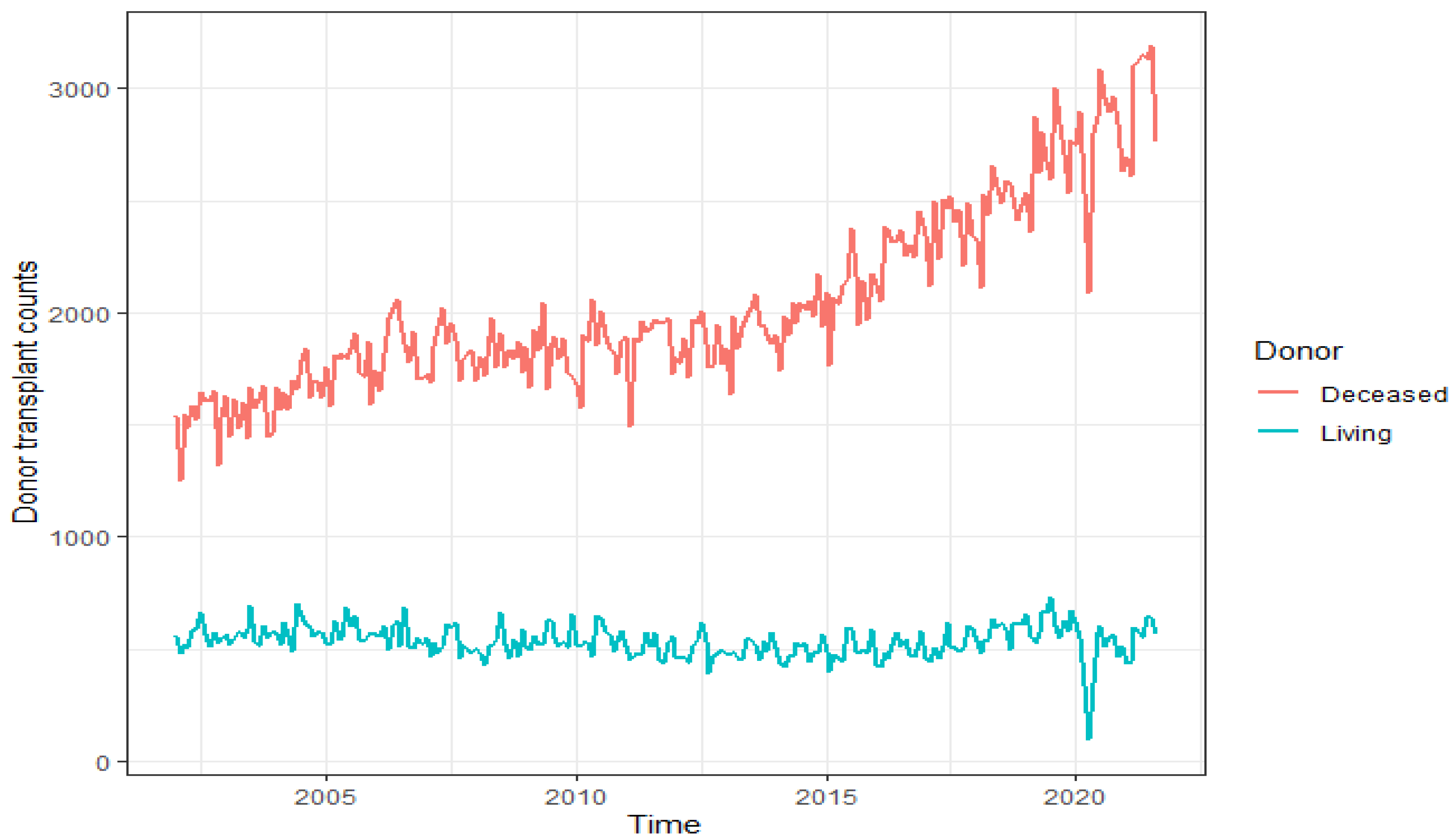
Donor transplant data consist of living and deceased donor type transplants. It is essential to maximize the number of living donors since it significantly decreases the wait time for patients in need of a transplant. It also helps people waiting for deceased donor organs by lowering the number of people on the waiting list. Living organ transplantation has many advantages over transplantation from a deceased donor [27]. Particularly for kidneys, the national wait time for a deceased donor kidney transplant can be as long as six years, and living donations significantly decrease the wait time for patients in need of a kidney transplant since the living kidney donor is often a close relative of the person getting the transplant, and there is a better chance of a good genetic match and less chance of rejection. As a result, living donor kidneys tend to last twice as long as deceased donor kidneys. Moreover, lower doses of immunosuppressive drugs may be used with fewer side effects. Figure 1 plots monthly counts of all donor transplants from 2002 to 2021 by donor type. The sudden fall in donor counts in March and subsequently in April 2020 was caused by the COVID-19 pandemic. It seems that the counts still did not go back completely to their prepandemic levels until August 2021.
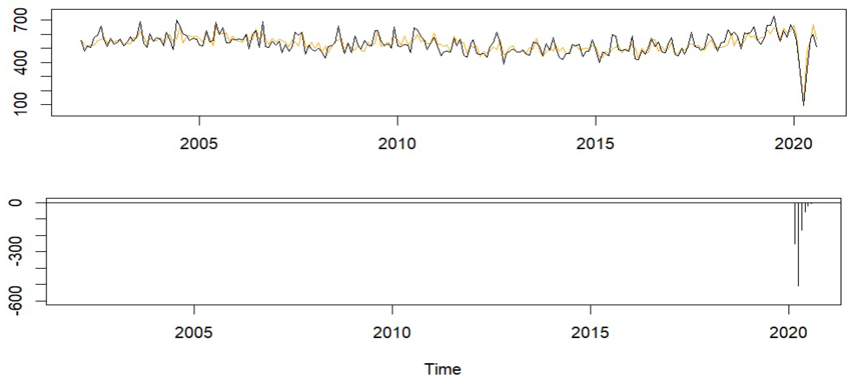
A SARIMA model with a period of 12 and the intervention effect in Equation (2) was fit to the living donor series up until August 2020. The monthly living donor transplant counts along with a model fit can be viewed in the top panel of Figure 2. The fitted model captured key features of the donor transplant counts fairly well, especially the effects of COVID-19, which are shown in the bottom panel of Figure 2. Notice that the COVID-19 pandemic caused a significant sudden change in the living donor transplant counts with a magnitude of −252.74 in March 2020. This further dropped to 509.71 in April 2020 followed by a gradual rebound at the rate of 33% to its pre-COVID level.
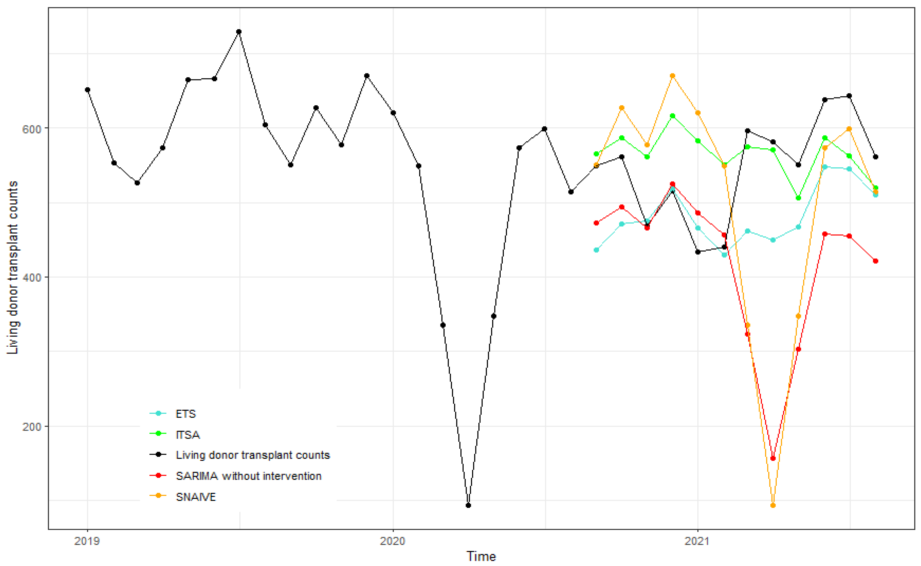
Figure 3 displays the living donor transplant counts from January 2019 to August 2021 and the forecasts from September 2020 to August 2021 using the ITSA model, SARIMA without intervention, ETS(M,N,A), and SNAIVE. Forecasts from ITSA and ETS performed similarly and were more accurate compared to those of SARIMA without intervention and SNAIVE. Living donor counts for the first six months were better forecasted using ETS and the latter ones using ITSA.
The accuracy measures are summarized in Table 1 for both living and deceased donor transplant time series at various forecast horizons. For example, the RMSE values of one-step-ahead forecasts were 72.78 and 68.39 for ITSA and ETS, respectively, which were much lower than the corresponding RMSE value of 192.28 from SNAIVE and a value of 113.19 from the SARIMA model forecasts without intervention. The estimated ITSA model parameters for both donor types are provided in Table A1 in the Appendix A.
Table 2 provides the results of the modified Diebold–Mariano test for equality of forecast accuracy comparing ITSA to ETS, SARIMA without intervention, and SNAIVE across forecast horizons one and four. A bold value indicates that the two forecasting methods were significantly different at the 10% level of significance. If the test statistic value is negative, then it shows that ITSA outperformed its competing method. For example, the DM test statistic was for the four-step-ahead forecasts of living donor counts comparing ITSA and SNAIVE, suggesting that ITSA performed significantly better compared to SNAIVE. Similarly, ETS outperformed ITSA for this example with .
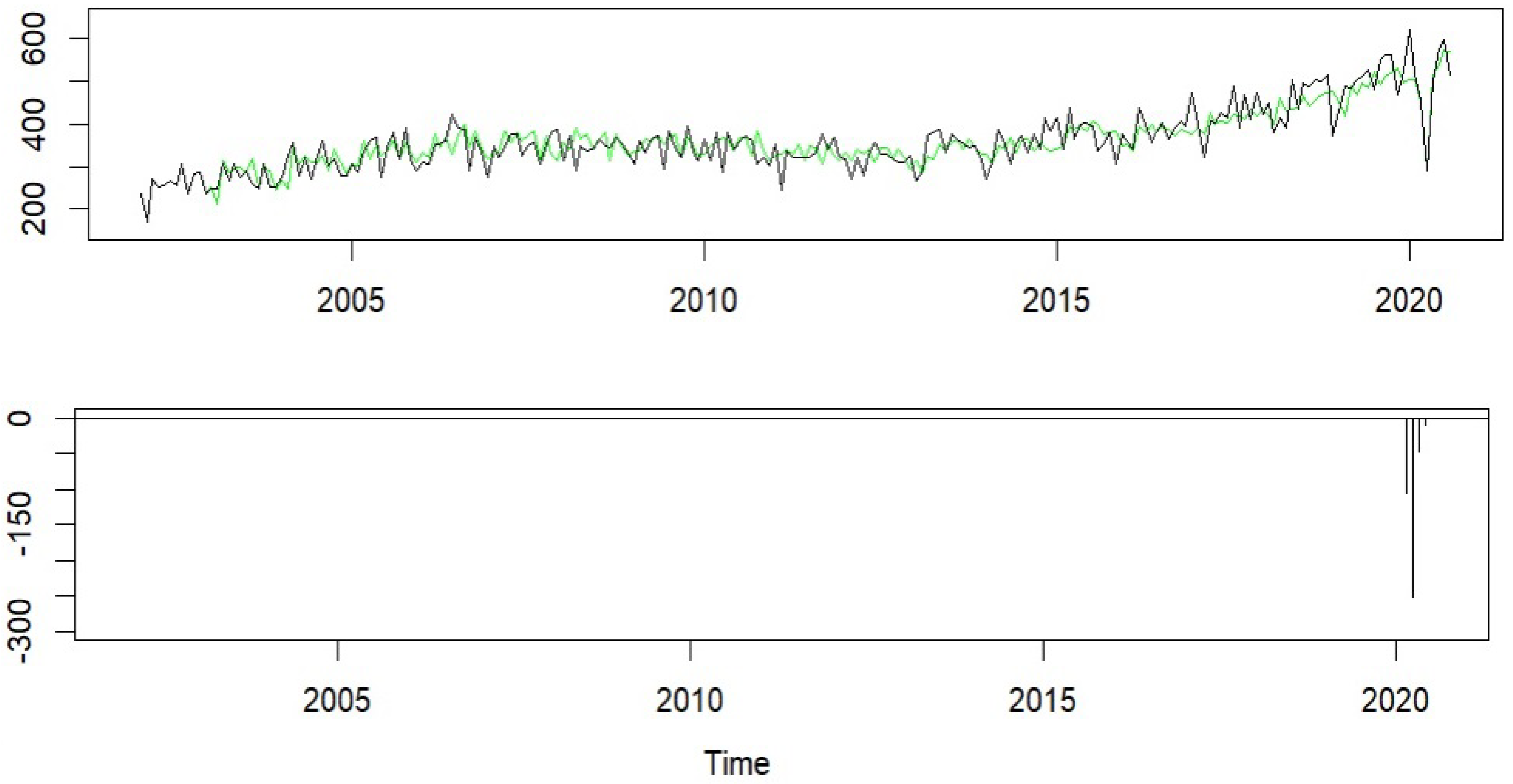
To further evaluate the forecasting performance of our ITSA model, we collected weekly metrics from the OPTN Metrics website [2] ranging from September 2021 to March 2022. Monthly living donor transplant counts were then obtained by summing the weekly donor counts for each month during this period. Here, the new calculated monthly living donor counts from September 2021 to March 2022 were treated as the test dataset and the donor counts from January 2002 to August 2021 as the training dataset.
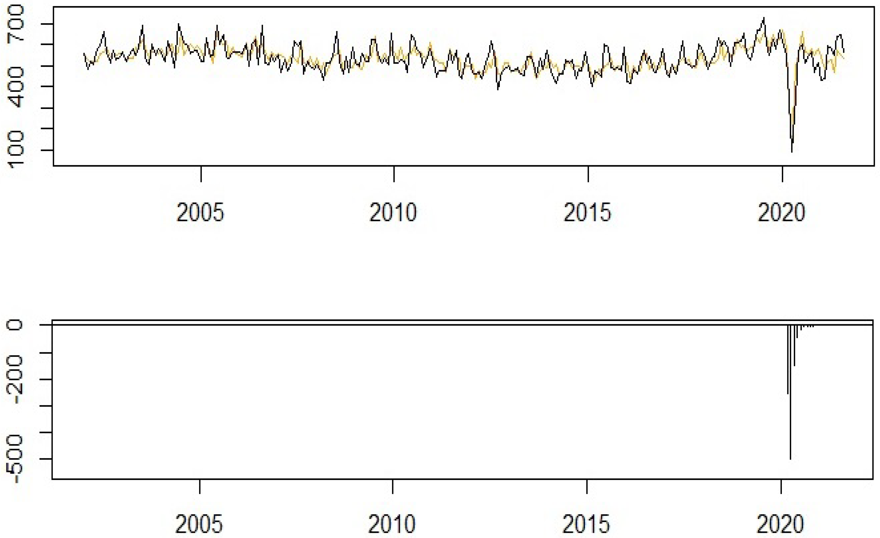
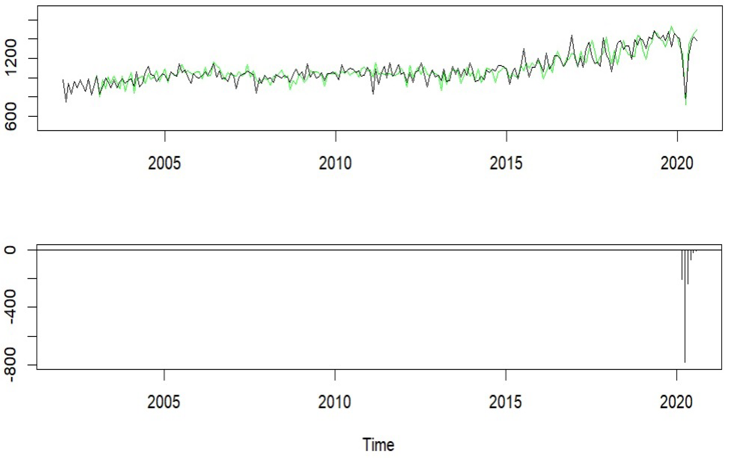
The fitted living donor counts with the training data are plotted in the top panel of Figure 4. Evidently, the ITSA model depicted the effects of the COVID-19 pandemic efficiently. The pandemic effects shown in the bottom panel of Figure 4 indicate that living donor transplants regained their losses after about two years after March 2020.
Forecasts for the test data are displayed in Figure 5 and matched up with the data reasonably well. In addition, the forecasts were not quite as volatile as the actual observations.
3.2. Organ
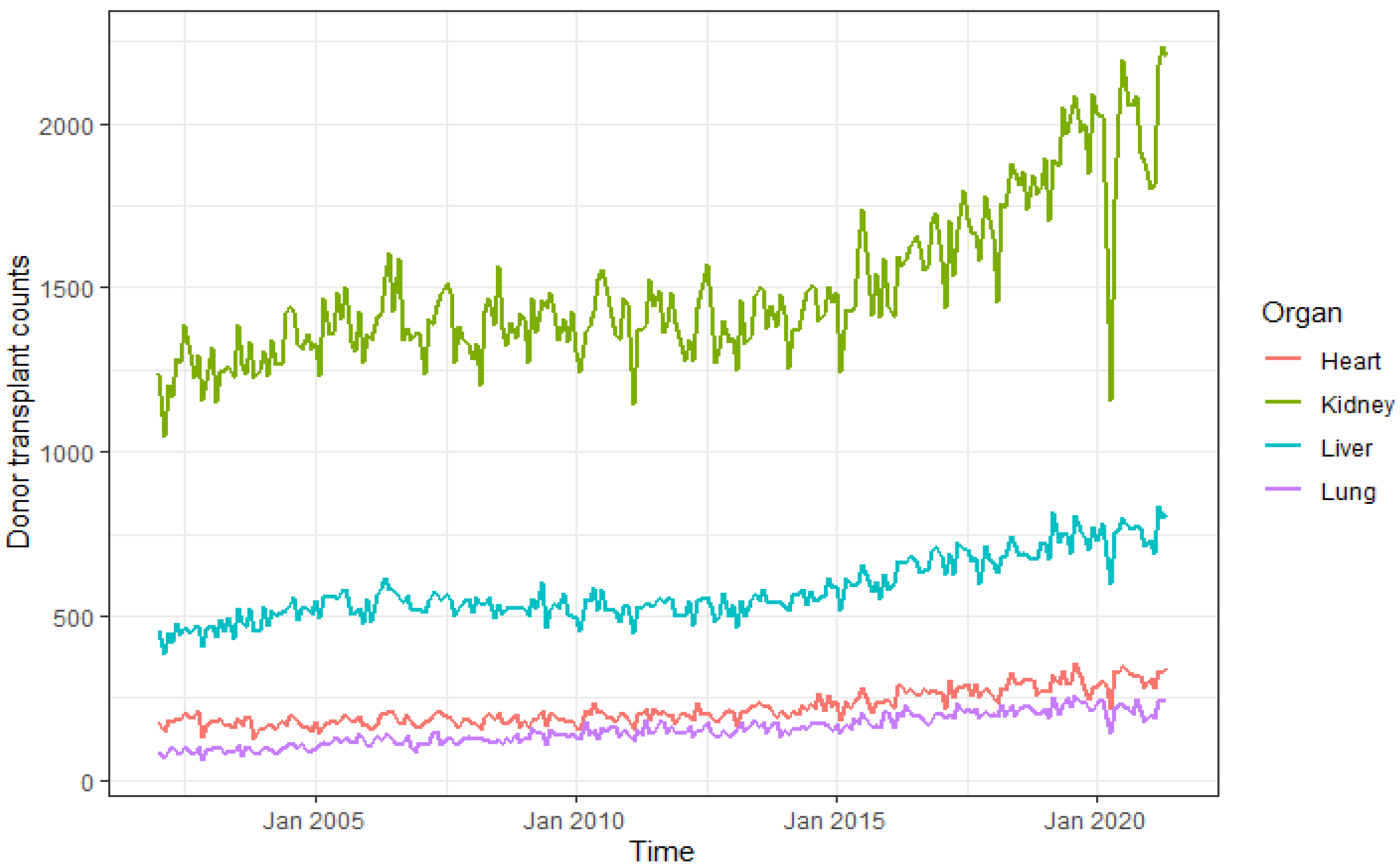
Heart, kidney, liver, and lung donor transplant counts were analyzed in our study. Figure 6 plots the monthly transplant counts of the four organs from both living and deceased donors. Apparently, the number of kidney donor transplants was affected most significantly by the COVID-19 pandemic, which is our focus here.
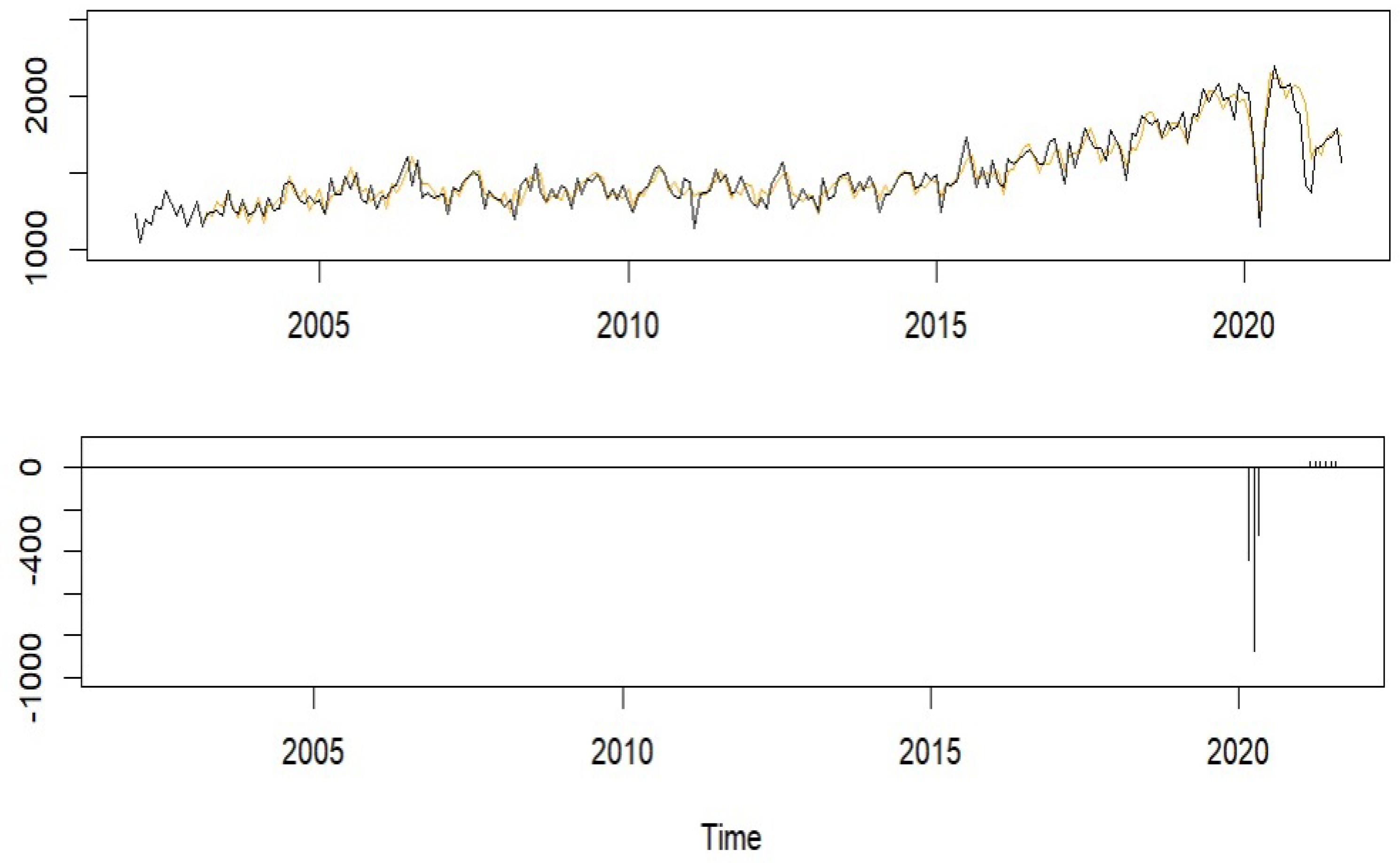
A SARIMA model with two intervention effects, namely, the occurrence of COVID-19 in March 2020 and the introduction of the kidney allocation policy in March 2021 in Equation (5) was fit to the kidney donor series from January 2002 to August 2021. The model fit plotted in the top panel of Figure 7 follows the observed kidney transplant trend very closely. The estimated effects of both COVID-19 and kidney allocation policy change are shown in the bottom panel of Figure 7.
As expected, the COVID-19 pandemic caused a significant sudden change in kidney donor transplant counts. The number of kidney donor transplants dropped by a magnitude of 438.85 in March 2020, 869.88 in April, and 317.91 in May. The effect of the kidney allocation policy appeared positive with a magnitude of 28.74, suggesting an increase in the number of kidney donor transplants due to the new kidney allocation policy. Given that only five months were included in the model fitting after the policy took effect, it was not surprising that its effect was insignificant.
In addition, for heart, liver, and lung donor transplant counts, we fit an ITSA model with only the COVID-19 pandemic as the intervention event. The estimated model parameters for all the organs focused on in this study are provided in Table A2 in the Appendix A.
Next, we compared the forecasts from September 2021 to April 2022 using the ITSA model with intervention events to those from SARIMA without intervention, ETS(M,A,M), and SNAIVE. All forecasts are plotted in Figure 8. Our method performed well, especially for the latter months of 2021.
Table 3 reports the MAPE and RMSE values for kidney, heart, liver, and lung at different forecast horizons. Overall, the model forecasts for heart and liver were better using ITSA, and ETS performed better for lung. For kidney, ITSA, SARIMA without intervention, and ETS performed similarly and were all better than SNAIVE.
The DM test results are summarized in Table 4 for organs. Overall, ITSA, ETS, and SARIMA without intervention generated comparable forecasts across all organs. For liver and kidney, ITSA performed significantly better than SNAIVE.
3.3. Age Group
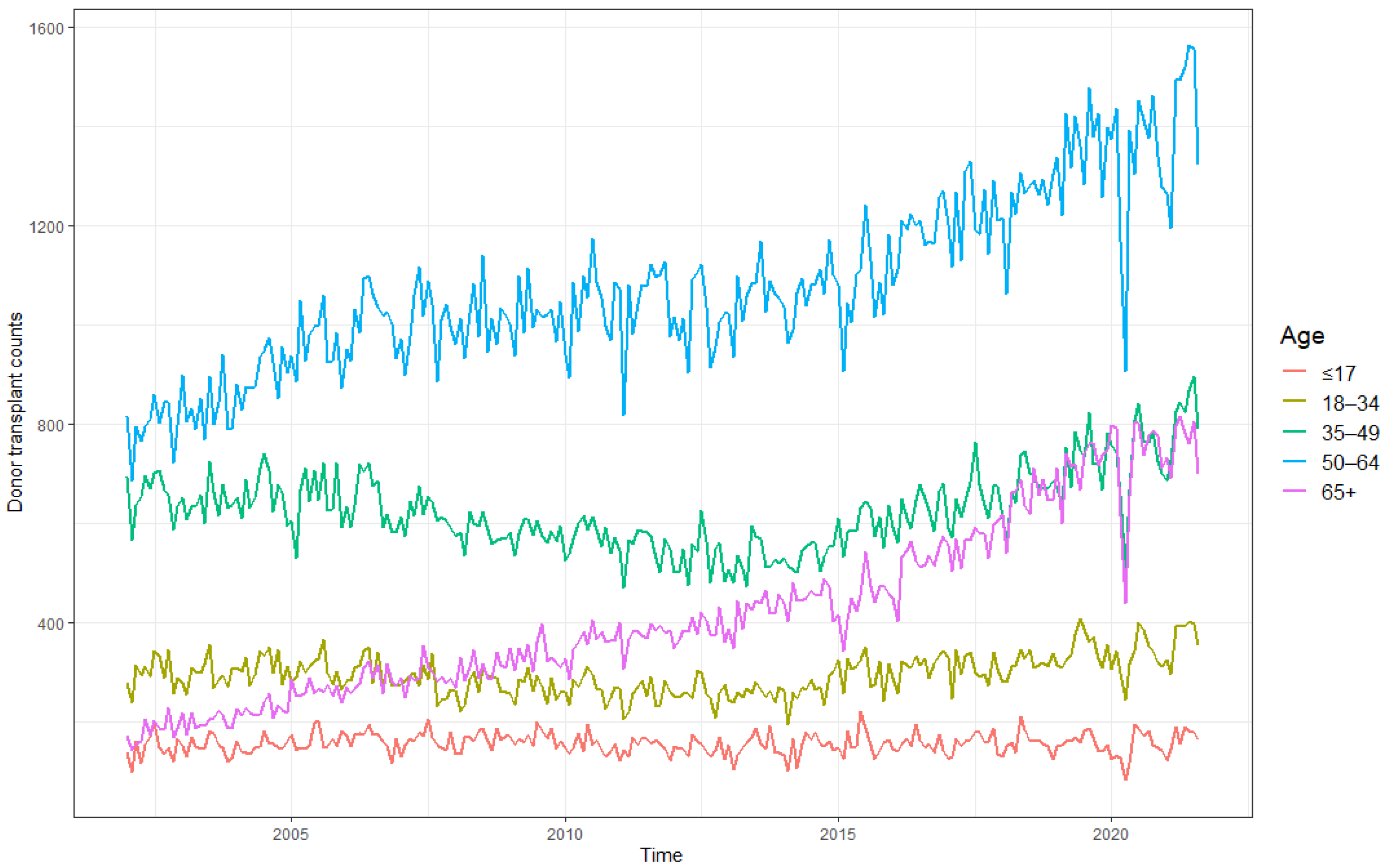
Donor age (including both living and deceased donors) was grouped into five intervals: 65+, 50–64, 35–49, 18–34, and ≤17. Figure 9 displays the monthly counts of all donor transplants performed in the US across the different age groups from January 2002 to August 2021. A significant drop in donor transplant counts around March 2020 was evident in all age groups, especially for ages over 35 years. It became noticeable early in the COVID-19 pandemic that older age was a risk factor for becoming severely ill with COVID-19. However, the virus’s impact on older adults went beyond a higher risk for serious infection. It may have been due to limited access to care for all health conditions, as well as considerable social and economic hardships [28]. Hence, in this subsection, our focus is on the 65+-year-old age group.
With the intervention effect in Equation (2), a SARIMA was fit to the 65+-year-old donor transplant counts. The model fit and the estimated COVID-19 effects are plotted in Figure 10. The COVID-19 pandemic caused a sudden change in the 65+-year-old donor transplant counts with a magnitude of −174.72 in March 2020. This further reduced to −321.13 in April 2020 followed by a faster rebound at a rate of 13% to its pre-COVID level. For all age groups, the estimated ITSA model parameters are provided in Table A3 in the Appendix A.
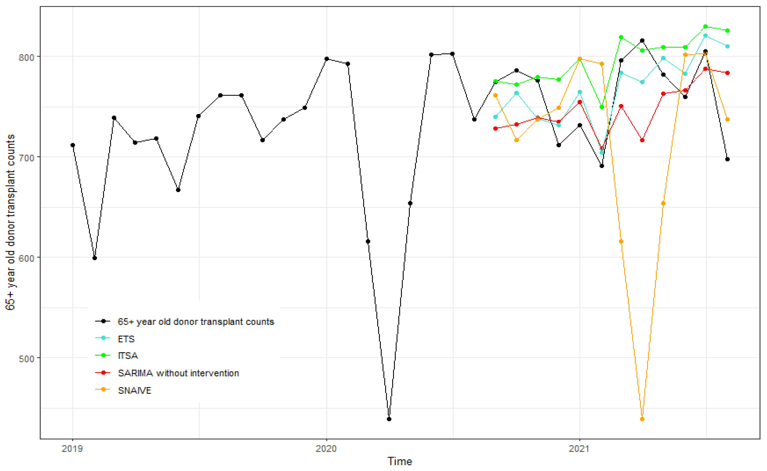
The forecasts generated for the 65+-year-old donor transplants from September 2020 to August 2021 are shown in Figure 11. ETS(M,A,M) was selected and performed better compared to other methods for the 65+-year-old age group. In addition, Table 5 summarizes the forecast accuracy measures for all age groups at various forecast horizons. The MAPE and RMSE values for ITSA were consistently lower than those for SARIMA without intervention, SNAIVE, and ETS for the 50–64-year-old age group.
The DM test results for age groups provided in Table 6 show that forecasts using ITSA were in general more accurate than those using the other three methods for almost all the age groups. However, this difference was not very significant. For the age group of ≤17, the DM statistic () was significant, implying that ITSA outperformed SNAIVE for the four-step-ahead forecasts.
3.4. Ethnicity
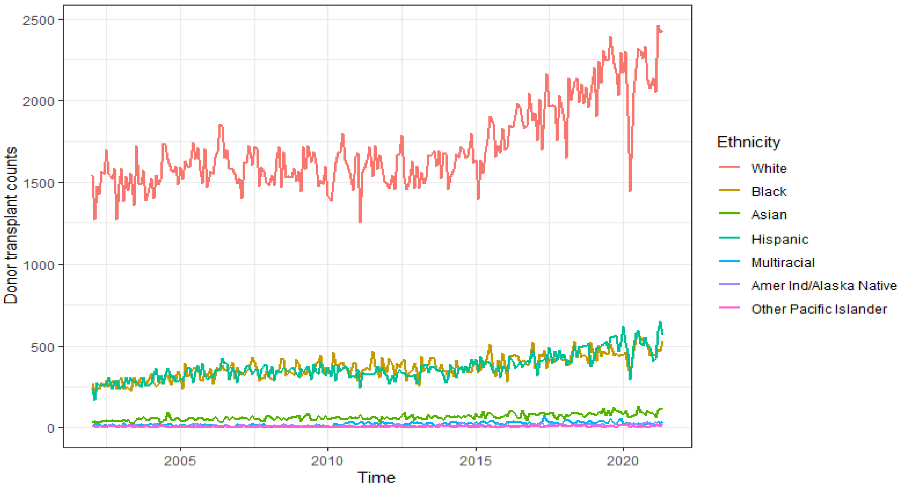
This section analyzes donor transplant counts from different ethnic groups. Figure 12 shows the monthly donor counts from White, Black, Asian, Hispanic, Multiracial, American Ind/Alaska Native, Native Hawaiian/other Pacific Islander. According to the analysis by the Institute for Health Metrics and Evaluation [29], Hispanic and Latino Americans were more likely to die from COVID-19 than non-Hispanic White Americans. The elevated risk in Hispanic, Latino, and non-Hispanic Black Americans meant that their risk of death at age 50 was equal to the risk of death for a 65-year-old non-Hispanic White American. This disparity could be attributed to several potential sources, including Hispanic and Latino populations’ increased work exposure during the pandemic [30]. Ethnic minorities on the transplant waitlist can get a better chance to find a good donor match if there is a more diverse donor registry since rare immune system markers match better for people from a similar ethnicity [31]. In 2019, Hispanics made up 18.4% of the national population. The number of organ transplants performed on Hispanics in 2020 was about 30% of the number of Hispanics currently waiting for a transplant. The number of transplants performed on Whites was 48.8% of the number currently waiting. While 20.5% of the total candidates currently waiting for transplants were Hispanic, they comprised 14.6% of organ donors in 2020. Almost 69% of organs recovered from Hispanic patients in 2020 were from deceased donors [32].
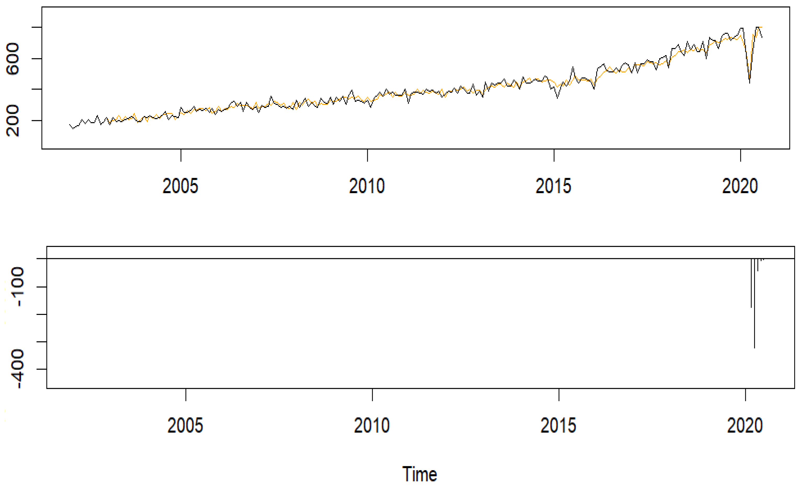
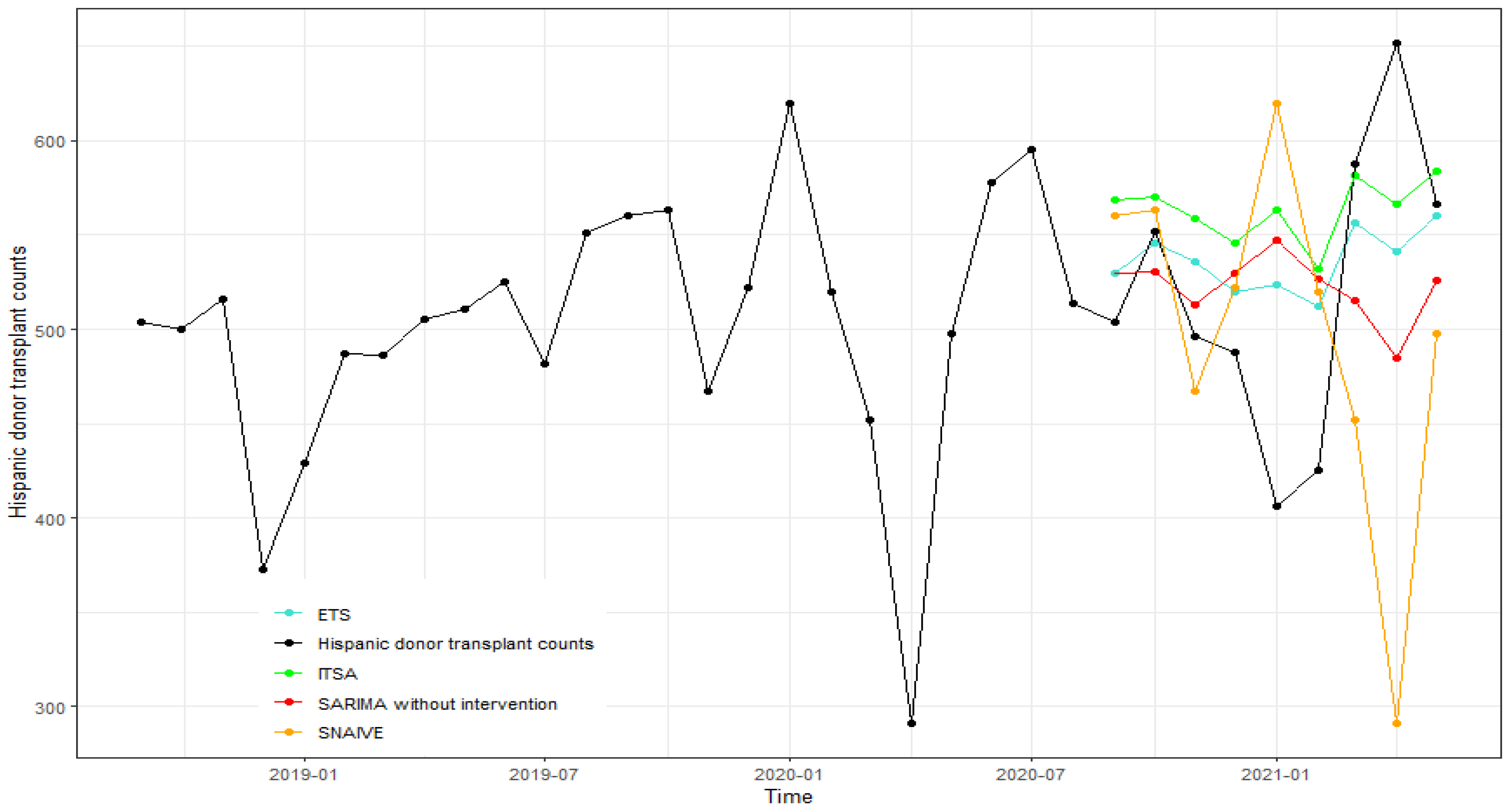
A SARIMA model with the COVID-19 intervention effect in Equation (2) was fit to the Hispanic donor transplant time series from January 2002 to August 2020. Monthly Hispanic donor transplant counts along with the model fit are plotted in the top panel of Figure 13. The bottom panel of Figure 13 shows the COVID-19 effects. The model fit the data quite well and the counts almost rebounded back gradually to their prepandemic levels by the summer of 2020. Specifically, the COVID-19 pandemic caused a sudden drop in Hispanic donor transplant counts by 104.34 in March 2020. This further dropped to −250.93 in April 2020 followed by a fast rebound at the rate of 19% to its pre-COVID level. The estimated ITSA model parameters for all the major ethnic categories focused on in our study are provided in Table A4 in the Appendix A.
The forecasts of Hispanic donor transplants from September 2022 to May 2021 generated using ITSA, SARIMA without intervention, ETS(M,Ad,A), and SNAIVE are shown in Figure 14. The overall forecasting ability of the ITSA model was good. ETS provided more accurate forecasts than the other three methods for the Hispanic donor transplant series. The MAPE and RMSE values of the major ethnic groups are reported in Table 7 for various forecast horizons. These measures were lower for the White population when using ITSA.
Table 8 provides the results of the modified Diebold–Mariano test for equality of forecast accuracy comparing ITSA to ETS, SARIMA without intervention, and SNAIVE across forecast horizons one and four by ethnicity. In general, ITSA generated better forecasts across the White, African American, and Asian population, when compared to the other three methods for the one-step-ahead forecasts as the test statistics were negative. In particular, ITSA forecasts were significantly better compared to SNAIVE for the Asian population. Other than that, there seemed to be no significant difference among all four methods in forecasting donor transplant counts by ethnicity.
3.5. Gender
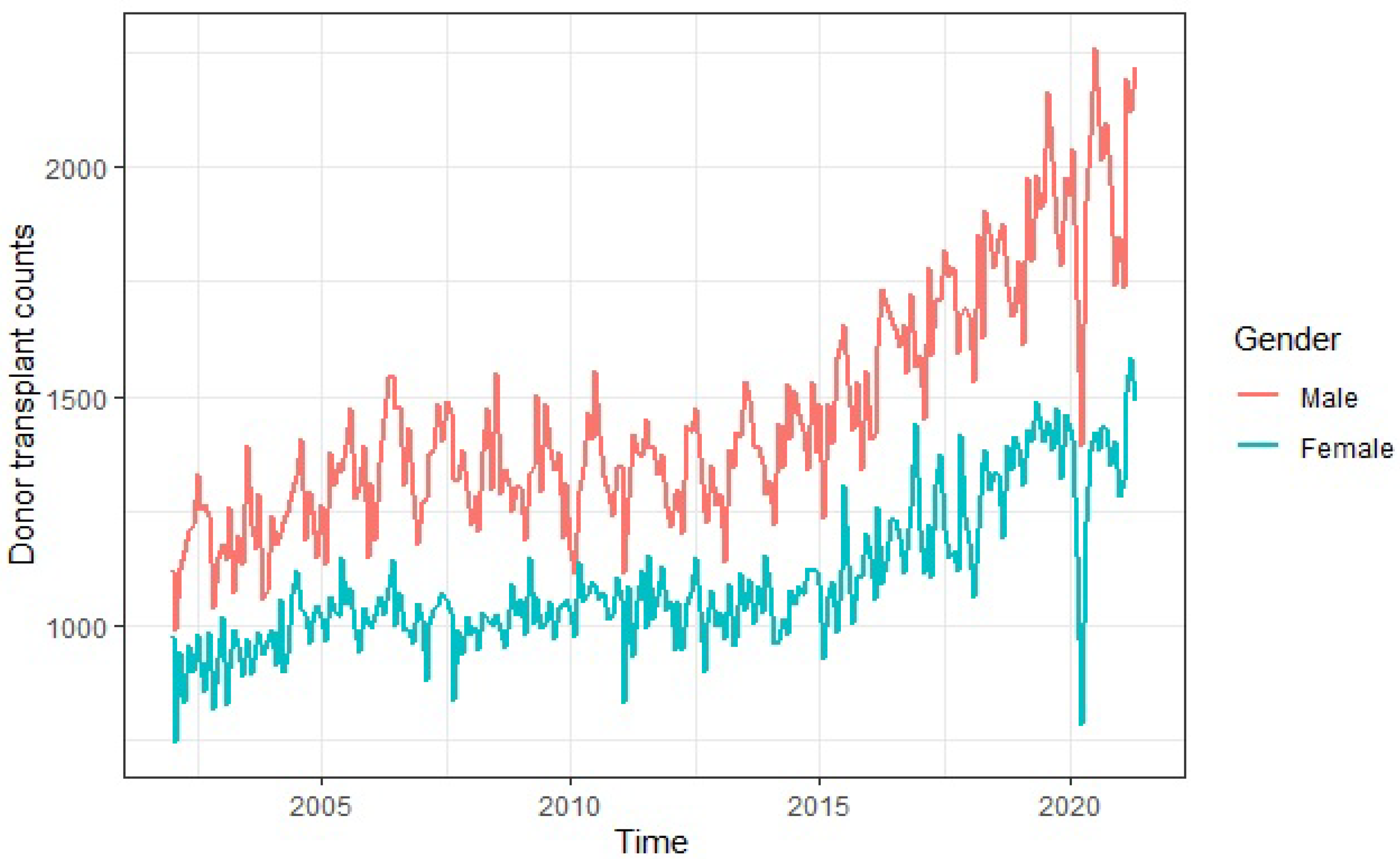
Gender disparities have always been prevalent in healthcare and continue to exist even in organ donation. Although organs in and of themselves are gender neutral and can be exchanged between the sexes, women account for up to two-thirds of all organ donations. Ref. [33] found no clear reasons why women were more willing to risk undergoing surgery than men and that their gender disparity was not mirrored in the demand for donated organs. More men than women are recipients, and women are less likely to complete the necessary steps to receive donated organs. Many research studies into diseases and treatments are skewed with a higher number of male participants, and conducting more research involving women can ensure women are properly represented in medical research. This will help alleviate gender bias [34]. Ref. [35] studied the impact of sex mismatch on transplant outcome and stated that it still remained a matter of debate. Their research found that sex and gender interaction could affect graft success and recommended that they should be taken into account in the management of organ-transplanted patients. In a national survey, both sexes had similar reasons for becoming and not becoming organ donor. However, compared with men, women were more willing to donate their organs to family members and strangers. Systematic changes and strategies to build trust in the medical system were also identified as means to change the stance of non-organ-donors from both sexes [36]. Figure 15 depicts donor transplant counts across male and female genders from January 2002 to May 2021 and the focus here was the female gender.
We fit a SARIMA with COVID-19 intervention in Equation (2) to the female donor transplant series from January 2002 to August 2020. The fitted donor counts and the estimated COVID-19 effects are plotted in Figure 16. As the above, the COVID-19 pandemic caused a sudden change in the female donor transplant counts with a magnitude of −208.36 in March 2020. This further dropped to a magnitude of 784.12 in April 2020 followed by a rebound at the rate of 30% to its pre-COVID level with no permanent effect. In addition, the ITSA model parameter estimates for both males and females are provided in Table A5 in the Appendix A.
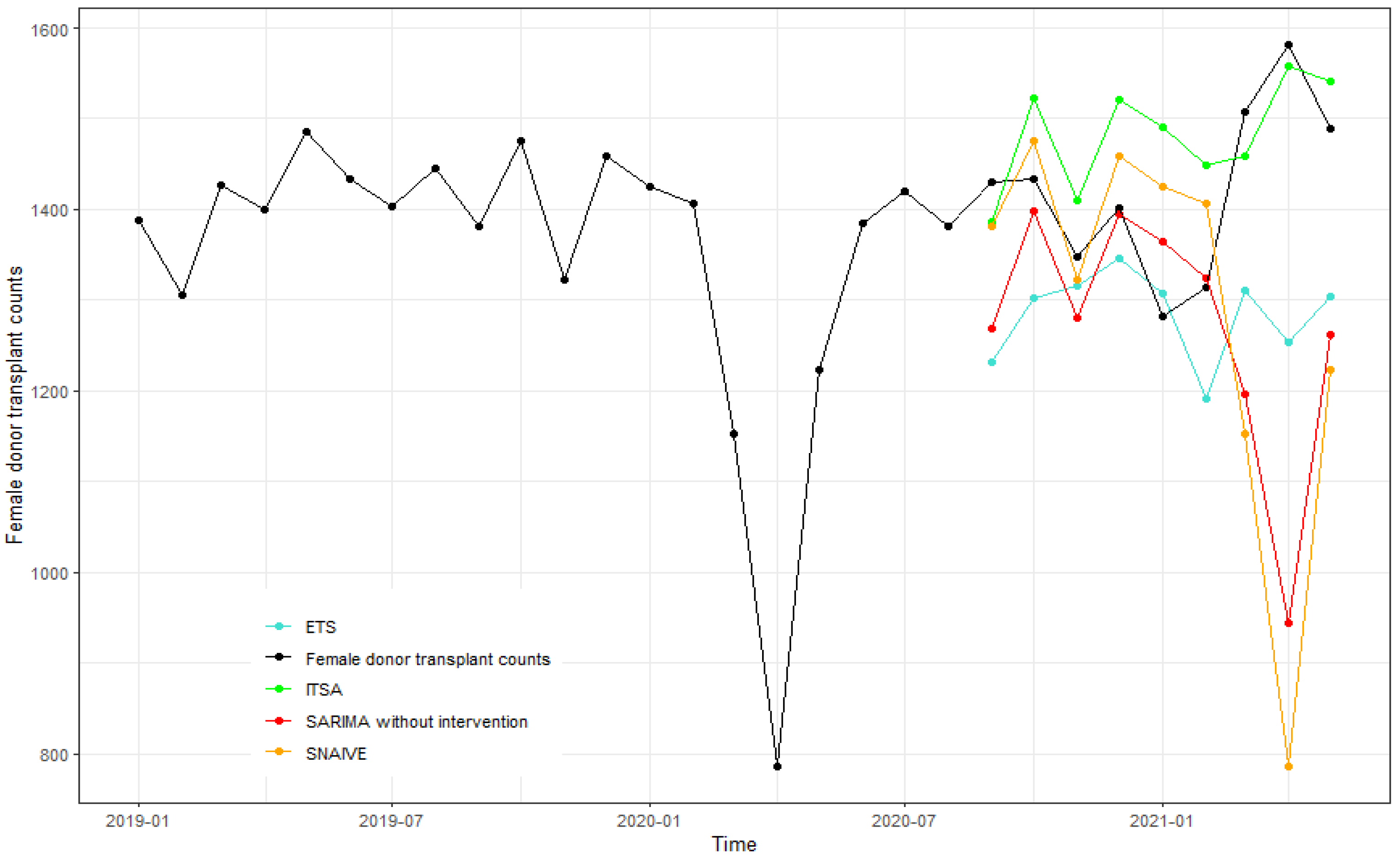
The forecasts of female donor counts from September 2020 to May 2021 are plotted in Figure 17 using ITSA, SARIMA without intervention, ETS(M,N,M), and SNAIVE. The forecasts using SARIMA without intervention were more accurate for the first six months and ITSA gave better forecasts for the latter months in 2021 for female donor counts. The forecast accuracy measures are reported in Table 9 for various forecast horizons. Both MAPE and RMSE values were generally lower for the ITSA model than SARIMA without intervention and SNAIVE. ETS seemed to perform equally to ITSA.
The DM test results for gender provided in Table 10 show that forecasts using ITSA are normally more accurate than those using SARIMA without intervention and SNAIVE for both males and females based on the negative values of the test statistic. However, this difference was not statistically significant.
4. Conclusions and Future Work
The occurrence of the COVID-19 pandemic provided an important research opportunity to investigate its nature and dynamics and our findings could help public health professionals and organizations mitigate risk when unanticipated situations arise in the future. The effects of COVID-19 on donor transplants could be well modeled with an intervention time series analysis. For all donor transplant series in the US, the significant drop caused by the COVID-19 pandemic in March 2020 is less than that in April 2020. This is because the OPTN Executive Committee issued a COVID-19 emergency policy that came into effect starting 17 March 2020 and donor transplant counts were affected thereafter.
The ITSA model forecast better when compared to the general SARIMA model without interventions and SNAIVE and performed similarly to ETS. The Diebold–Mariano tests did not show as many significant differences among the forecast methods compared in the study as we had expected. Since the sample sizes in each of the DM tests were small, the DM tests need to be used with caution.
This study can easily be extended to forecast waitlist registrations and organ transplant counts with different intervention events. It can also be utilized by policymakers to examine the impact of policies and practices to improve equity metrics in the organ transplant system.
Note that there are many other factors across the individual biological/healthcare system/community that contribute to inequities among donor transplant candidates. They were not addressed since the scope of this study spanned only across individual sociocultural factors. In a future study, the combined effects of all factors mentioned above on donor transplant count time series can be evaluated in a mixed multi-way time series analysis of covariance (ANCOVA) with intervention effects. For example, if we want to study the combined effects of gender and ethnicity on the living kidney donor count time series, a two-way time series ANCOVA model with an intervention effect can be developed as follows:
where is the observed donor count at time t for the ith level of gender and jth level of ethnicity. includes trend and/or seasonality components, is the intervention effect, is the gender effect, and is the ethnicity effect. The error term is assumed to be mean zero stationary time series. This model format is similar to the one in [37].
The parameter estimation and forecasts for the proposed time series ANCOVA model are quite challenging. Recently, a hybrid model, which combines both statistical and machine learning components has been gaining popularity in time series forecasting as it outperforms either pure traditional statistical methods or pure machine learning methods [38,39]. The hybrid method of the proposed time series ANCOVA model and deep neural networks seems an appealing approach to time series forecasting.
Author Contributions
S.M. and Q.L. have contributed equally to this work. All authors have read and agreed to the published version of the manuscript.
Funding
This research received no external funding.
Data Availability Statement
Yearly data on transplants are available here: https://optn.transplant.hrsa.gov/data/view-data-reports/ (accessed on 10 March 2021). Monthly data on transplants as presented in this study are available on request from the corresponding author. The data are not publicly available due to a signed data usage agreement with the United Network for Organ Sharing (UNOS).
Acknowledgments
We would like to sincerely thank the UNOS for providing us with the data required for the study.
Conflicts of Interest
The authors declare no conflict of interest.
Appendix A

Table A1.
ITSA model parameter estimates for donor types.
| Donor Type | ||
|---|---|---|
| Coefficients | Living | Deceased |
| −0.66 | ||
| −0.07 | −0.80 | |
| −0.75 | ||
| 0.60 | −1.50 | |
| 0.25 | 0.56 | |
| −252.74 | −559.54 | |
| 0.33 | 0.15 | |
| −509.71 | −787.22 | |
Table A2.
ITSA model parameter estimates for organs.
| Organ | ||||
|---|---|---|---|---|
| Coefficients | Heart | Liver | Lung | Kidney |
| −0.87 | −0.78 | −0.81 | −0.59 | |
| 0.04 | ||||
| −0.74 | −0.81 | 0.27 | −0.87 | |
| −42.21 | −107.91 | −50.18 | −438.85 | |
| 0.04 | 0.1 | 0.21 | ||
| −88.75 | −163.80 | −78.21 | −869.88 | |
| −317.91 | ||||
| 28.74 | ||||
Table A3.
ITSA model parameter estimates for age groups.
| Age Group | |||||
|---|---|---|---|---|---|
| Coefficients | 65+ | 50–64 | 35–49 | 18–34 | |
| −0.16 | |||||
| −0.64 | −0.82 | −0.81 | −0.83 | −0.90 | |
| −0.11 | −0.06 | ||||
| −0.37 | −0.61 | 0.37 | |||
| −0.26 | 0.15 | ||||
| −0.86 | −0.98 | ||||
| −174.72 | −239.65 | −112.85 | −60.55 | −29.93 | |
| 0.13 | 0.06 | 0.23 | 0.45 | 0.30 | |
| −321.13 | −448.44 | −265.88 | −114.28 | −77.29 | |
Table A4.
ITSA model parameter estimates for ethnicity.
| Ethnicity | ||||
|---|---|---|---|---|
| Coefficients | White | Black | Hispanic | Asian |
| −0.83 | −0.99 | −0.82 | −0.89 | |
| −0.06 | ||||
| −0.78 | −0.90 | −0.85 | 0.14 | |
| −386.83 | −149.97 | −104.34 | −27.18 | |
| 0.22 | 0.46 | 0.19 | 0.41 | |
| −768.97 | −196.54 | −250.93 | −31.22 | |
Table A5.
ITSA model parameter estimates for gender.
| Gender | ||
|---|---|---|
| Coefficients | Female | Male |
| −0.16 | ||
| −0.87 | −0.79 | |
| −0.46 | ||
| −0.74 | ||
| −0.02 | ||
| −208.36 | −326.80 | |
| 0.30 | 0.02 | |
| −784.12 | −613.78 | |
References
- The Urgent Need to Reform the Organ Transplantation System to Secure More Organs for Waiting, Ailing, and Dying Patients. Available online: https://oversight.house.gov/legislation/hearings/the-urgent-need-to-reform-the-organ-transplantation-system-to-secure-more (accessed on 4 July 2021).
- OPTN Metrics. Available online: https://insights.unos.org/OPTN-metrics/ (accessed on 2 April 2021).
- Loupy, A.; Aubert, O.; Reese, P.P.; Bastien, O.; Bayer, F.; Jacquelinet, C. Organ procurement and transplantation during the COVID-19 pandemic. Lancet 2020, 395, E95–E96. [Google Scholar] [CrossRef]
- All-Time Records Again Set in 2021 for Organ Transplants, Organ Donation from Deceased Donors. Available online: https://unos.org/news/2021-all-time-records-organ-transplants-deceased-donor-donation/ (accessed on 2 January 2021).
- Cisterna-García, A.; Guillén-Teruel, A.; Caracena, M.; Pérez, E.; Jiménez, F.; Francisco-Verdú, F.J.; Reina, G.; González-Billalabeitia, E.; Palma, J.; Sánchez-Ferrer, Á.; et al. A predictive model for hospitalization and survival to COVID-19 in a retrospective population-based study. Sci. Rep. 2022, 12, 18126. [Google Scholar] [CrossRef]
- Ramallo-González, A.P.; González-Vidal, A.; Skarmeta, A.F. CIoTVID: Towards an Open IoT-Platform for Infective Pandemic Diseases such as COVID-19. Sensors 2021, 21, 484. [Google Scholar] [CrossRef]
- New Kidney, Pancreas Allocation Policies in Effect. OPTN News Room. Available online: https://optn.transplant.hrsa.gov/news/new-kidney-pancreas-allocation-policies-in-effect/#:~:text=Effective%20March%2015%2C%202021%2C%20the,transplant%20access%20for%20candidates%20nationwide (accessed on 21 April 2021).
- Bordes, S.J.; Montorfano, L.; West-Ortiz, W.; Valera, R.; Cracco, A.; Alonso, M.; Pinna, A.D.; Ebaid, S. Trends in US Kidney Transplantation During the COVID-19 Pandemic. Cureus 2020, 12, e12075. [Google Scholar] [CrossRef]
- Suarez-Pierre, A.; Choudhury, R.; Carroll, A.M.; King, R.W.; Iguidbashian, J.; Cotton, J.; Colborn, K.L.; Kennealey, P.T.; Cleveland, J.C.; Pomfret, E.; et al. Measuring the effect of the COVID-19 pandemic on solid organ transplantation. Am. J. Surg. 2021, 224, 437–442. [Google Scholar] [CrossRef]
- Gerlach, A.L. Increasing Organ Donations in Maryland: An Interrupted Time Series Analysis. Ph.D. Thesis, Walden University, Minneapolis, MN, USA, 2018. [Google Scholar]
- Hudson, J.; Fielding, S.; Ramsay, C.R. Methodology and reporting characteristics of studies using interrupted time series design in healthcare. BMC Med. Res. Methodol. 2019, 19, 137. [Google Scholar] [CrossRef] [Green Version]
- Schaffer, A.L.; Dobbins, T.A.; Pearson, S.A. Interrupted time series analysis using autoregressive integrated moving average (ARIMA) models: A guide for evaluating large-scale health interventions. BMC Med. Res. Methodol. 2021, 21, 58. [Google Scholar] [CrossRef]
- Morales, D.R.; Morant, S.V.; MacDonald, T.M.; Hallas, J.; Ernst, M.T.; Pottegard, A.; Herings, R.M.; Smits, E.; Overbeek, J.A.; Mackenzie, I.S.; et al. Impact of EU regulatory label changes for diclofenac in people with Cardiovascular disease in four countries: Interrupted time series regression analysis. Br. J. Clin Pharmacol. 2020, 1–12. [Google Scholar] [CrossRef]
- Jandoc, R.; Burden, A.M.; Mamdani, M.; Lévesque, L.E.; Cadarette, S.M. Interrupted time series analysis in drug utilization research is increasing: Systematic review and recommendations. J. Clin. Epidemiol. 2015, 68, 950–956. [Google Scholar] [CrossRef] [Green Version]
- Data Dashboard Monitors Equity in Access to Transplant. Available online: https://unos.org/news/insights/equity-in-access-to-transplant-dashboard/ (accessed on 5 July 2021).
- Disparity Persists: Racial and Ethnic Minority Patients Still Less Likely than White Patients to Get Live Donor Kidney Transplants. Available online: https://www.hopkinsmedicine.org/news/newsroom/news-releases/disparity-persists-racial-and-ethnic-minority-patients-still-less-likely-than-white-patients-to-get-live-donor-kidney-transplants (accessed on 18 August 2021).
- Park, C.; Jones, M.M.; Kaplan, S.; Koller, F.L.; Wilder, J.M.; Boulware, L.; McElroy, L.M. A scoping review of inequities in access to organ transplant in the United States. Int. J. Equity Health 2022, 21, 22. [Google Scholar] [CrossRef]
- Organ Procurement and Transplantation Network. Available online: http://optn.transplant.hrsa.gov (accessed on 8 March 2021).
- Box, G.E.P.; Tiao, G.C. Intervention Analysis with Applications to Economic and Environmental Problems. J. Am. Stat. Assoc. 1975, 70, 70–90. [Google Scholar] [CrossRef]
- Cryer, J.D.; Chan, K. Time Series Analysis with Applications in R; Springer: Berlin/Heidelberg, Germany, 2008. [Google Scholar]
- Hyndman, R.J.; Koehler, A.B.; Snyder, R.D.; Grose, S. A state space framework for automatic forecasting using exponential smoothing methods. Int. J. Forecast. 2002, 18, 439–454. [Google Scholar] [CrossRef] [Green Version]
- Hyndman, R.J.; Koehler, A.B.; Ord, J.K.; Snyder, R.D. Forecasting with Exponential Smoothing: The State Space Approach; Springer: Berlin/Heidelberg, Germany, 2008. [Google Scholar]
- Holt, C.E. Forecasting Seasonals and Trends by Exponentially Weighted Averages (O.N.R. Memorandum No. 52); Carnegie Institute of Technology: Pittsburgh, PA, USA, 1957. [Google Scholar]
- Winters, P.R. Forecasting sales by exponentially weighted moving averages. Manag. Sci. 1960, 6, 324–342. [Google Scholar] [CrossRef]
- Diebold, F.X.; Mariano, R.S. Comparing predictive accuracy. J. Bus. Econ. Stat. 1995, 13, 253–263. [Google Scholar]
- Harvey, D.; Leybourne, S.; Newbold, P. Testing the equality of prediction mean squared errors. Int. J. Forecast. 1997, 13, 281–291. [Google Scholar] [CrossRef]
- Living kidney Donation. Hume-Lee Transplant Center. Available online: https://www.vcuhealth.org/hume-lee-transplant-center/living-donation/living-kidney-donation (accessed on 6 May 2021).
- Williams, I.R.; Shah, A.; Doty, M.; Fields, K.; FitzGerald, M. The Impact of COVID-19 on Older Adults: Findings from the 2021 International Health Policy Survey of Older Adults. Commonw. Fund 2021. [Google Scholar] [CrossRef]
- Institute for Health Metrics and Evaluation. Available online: https://www.healthdata.org/ (accessed on 25 February 2021).
- Examining the Impact: COVID-19 and the Hispanic Community. Available online: https://www.healthdata.org/acting-data/examining-impact-COVID-19-and-hispanic-community (accessed on 15 October 2021).
- Organ Donation Statistics. Available online: https://www.organdonor.gov/learn/organ-donation-statistics (accessed on 10 April 2022).
- Organ Donation and Hispanic Americans. US Department of Health and Human Services Office of Minority Health. Available online: https://minorityhealth.hhs.gov/omh/browse.aspx?lvl=4&lvlid=72 (accessed on 22 January 2022).
- Steinman, J.L. Gender disparity in organ donation. Gend. Med. 2006, 3, 246–252. [Google Scholar] [CrossRef]
- Exploring Gender Bias in Healthcare. Available online: https://www.fiercehealthcare.com/sponsored/exploring-gender-bias-healthcare (accessed on 16 April 2021).
- Puoti, F.; Ricci, A.; Nanni-Costa, A.; Ricciardi, W.; Malorni, W.; Ortona, E. Organ transplantation and gender differences: A paradigmatic example of intertwining between biological and sociocultural determinants. Biol Sex Differ 2016, 7, 35. [Google Scholar] [CrossRef] [Green Version]
- Yee, E.; Hosseini, S.M.; Duarte, B.; Knapp, S.M.; Carnes, M.; Young, B.; Sweitzer, N.K.; Breathett, K. Sex Disparities in Organ Donation: Finding an Equitable Donor Pool. J. Am. Heart Assoc. 2021, 10, e020820. [Google Scholar] [CrossRef]
- Azimmohseni, M.; Khalafi, M.; Kordkatuli, M. Time series analysis of 5covariance based on linear transfer function models. Stat. Inference Stoch. Process. 2019, 22, 1–16. [Google Scholar] [CrossRef]
- Smyl, S. A hybrid method of exponential smoothing and recurrent neural networks for time series forecasting. Int. J. Forecast. 2020, 36, 75–85. [Google Scholar] [CrossRef]
- Lim, B.; Zohren, S. Time-series forecasting with deep learning: A survey. Philos. Trans. R. Soc. 2021, 379, 20200209. [Google Scholar] [CrossRef]
Figure 1.
Donor transplant counts in the US by donor type, based on OPTN data as of November 2021.

Figure 2.
Living donor transplant counts with the model fit (top) and the estimated COVID-19 effects (bottom).
Figure 2.
Living donor transplant counts with the model fit (top) and the estimated COVID-19 effects (bottom).

Figure 3.
Forecasts of living donor transplant counts from September 2020 to August 2021 using ITSA, SARIMA without intervention, ETS, and SNAIVE.
Figure 3.
Forecasts of living donor transplant counts from September 2020 to August 2021 using ITSA, SARIMA without intervention, ETS, and SNAIVE.

Figure 4.
Living donor transplant counts (January 2002 to August 2021) with the model fit (top) and the estimated COVID-19 effects (bottom).
Figure 4.
Living donor transplant counts (January 2002 to August 2021) with the model fit (top) and the estimated COVID-19 effects (bottom).

Figure 5.
Forecasts of living donors from September 2021 to March 2022.

Figure 6.
Donor transplant counts in the US by organ, based on OPTN data as of November 2021.

Figure 7.
Kidney donor transplant counts with the model fit (top) and the estimated COVID-19 effects (bottom).
Figure 7.
Kidney donor transplant counts with the model fit (top) and the estimated COVID-19 effects (bottom).

Figure 8.
Forecasts of kidney donor transplant counts from September 2021 to April 2022 using ITSA, SARIMA without intervention, ETS, and SNAIVE.
Figure 8.
Forecasts of kidney donor transplant counts from September 2021 to April 2022 using ITSA, SARIMA without intervention, ETS, and SNAIVE.

Figure 9.
All donor transplant counts in the US across different age groups, based on OPTN data as of November 2021.
Figure 9.
All donor transplant counts in the US across different age groups, based on OPTN data as of November 2021.

Figure 10.
Donor transplant counts for the 65+-year-old group with the model fit (top) and the estimated COVID-19 effects (bottom).
Figure 10.
Donor transplant counts for the 65+-year-old group with the model fit (top) and the estimated COVID-19 effects (bottom).

Figure 11.
Forecasts of all donor transplant counts for the 65+-year-old from September 2020 to August 2021 using ITSA, SARIMA without intervention, ETS, and SNAIVE.
Figure 11.
Forecasts of all donor transplant counts for the 65+-year-old from September 2020 to August 2021 using ITSA, SARIMA without intervention, ETS, and SNAIVE.

Figure 12.
Donor transplant counts in the US across ethnicity, based on OPTN data as of November 2021.
Figure 12.
Donor transplant counts in the US across ethnicity, based on OPTN data as of November 2021.

Figure 13.
Hispanic donor transplant counts with the model fit (top) and the estimated COVID-19 effects (bottom).
Figure 13.
Hispanic donor transplant counts with the model fit (top) and the estimated COVID-19 effects (bottom).

Figure 14.
Forecasts of the Hispanic donor transplants from September 2020 to May 2021 using ITSA, SARIMA without intervention, ETS, and SNAIVE.
Figure 14.
Forecasts of the Hispanic donor transplants from September 2020 to May 2021 using ITSA, SARIMA without intervention, ETS, and SNAIVE.

Figure 15.
Donor transplant counts in the US across gender, based on OPTN data as of November 2021.

Figure 16.
Female donor transplant counts with the model fit (top) and the estimated COVID-19 effects (bottom).
Figure 16.
Female donor transplant counts with the model fit (top) and the estimated COVID-19 effects (bottom).

Figure 17.
Forecasts of female donor transplants from September 2020 to May 2021 using ITSA, SARIMA without intervention, ETS, and SNAIVE.
Figure 17.
Forecasts of female donor transplants from September 2020 to May 2021 using ITSA, SARIMA without intervention, ETS, and SNAIVE.

Table 1.
Forecast accuracy measures by donor type at various forecast horizons.
| h | MAPE (%) | RMSE | |||
|---|---|---|---|---|---|
| Living | Deceased | Living | Deceased | ||
| ITSA | 1 | 12.16 | 5.46 | 72.78 | 191.79 |
| 2 | 16.76 | 6.08 | 93.09 | 210.46 | |
| 4 | 18.95 | 7.64 | 104.88 | 232.60 | |
| 8 | 9.58 | 3.97 | 65.78 | 183.95 | |
| SARIMA | 1 | 13.49 | 6.27 | 113.19 | 235.95 |
| 2 | 21.53 | 7.45 | 171.14 | 262.09 | |
| 4 | 26.73 | 8.22 | 195.57 | 274.17 | |
| 8 | 37.20 | 8.08 | 244.44 | 303.53 | |
| ETS | 1 | 10.28 | 4.94 | 68.39 | 178.38 |
| 2 | 10.57 | 6.09 | 69.86 | 204.10 | |
| 4 | 10.48 | 6.60 | 71.19 | 217.95 | |
| 8 | 11.45 | 7.39 | 76.62 | 240.55 | |
| SNAIVE | 1 | 26.94 | 10.06 | 192.28 | 398.95 |
| 2 | 29.35 | 10.81 | 200.83 | 416.41 | |
| 4 | 32.01 | 11.03 | 217.98 | 440.09 | |
| 8 | 29.25 | 12.63 | 240.27 | 513.26 | |
Table 2.
Results of the modified Diebold–Mariano test comparing ITSA to ETS, SARIMA without intervention, and SNAIVE by donor type.
Table 2.
Results of the modified Diebold–Mariano test comparing ITSA to ETS, SARIMA without intervention, and SNAIVE by donor type.
| Donor Type | h | ETS | SARIMA | SNAIVE |
|---|---|---|---|---|
| Living | 1 | 0.32 | −1.11 | −1.66 |
| 4 | 3.52 | −1.47 | −2.25 | |
| Deceased | 1 | 0.46 | −1.12 | 1.40 |
| 4 | 0.14 | −0.86 | −1.19 |
Bold indicates a statistical difference between the two forecasting methods at the 10% level of significance. Negative (positive) values indicate that ITSA performed better (worse) than ETS, SARIMA without intervention, or SNAIVE.
Table 3.
Forecast accuracy measures by organ type at various forecast horizons.
| h | MAPE (%) | RMSE | |||||||
|---|---|---|---|---|---|---|---|---|---|
| Heart | Liver | Lung | Kidney | Heart | Liver | Lung | Kidney | ||
| ITSA | 1 | 3.69 | 5.50 | 11.68 | 9.97 | 13.94 | 55.40 | 27.19 | 181.45 |
| 2 | 3.45 | 6.37 | 12.13 | 9.73 | 13.64 | 64.03 | 28.57 | 178.25 | |
| 4 | 3.63 | 7.67 | 14.16 | 11.23 | 14.23 | 79.37 | 31.07 | 182.16 | |
| 8 | 3.13 | 9.36 | 7.23 | - | 11.27 | 88.98 | 16.97 | - | |
| SARIMA | 1 | 4.64 | 6.11 | 11.73 | 9.46 | 18.06 | 60.76 | 30.39 | 166.30 |
| 2 | 4.92 | 7.28 | 13.03 | 10.28 | 19.03 | 71.05 | 33.79 | 170.12 | |
| 4 | 4.94 | 8.79 | 15.33 | 12.37 | 19.50 | 89.14 | 35.92 | 194.96 | |
| 8 | 5.36 | 11.77 | 11.92 | - | 23.02 | 110.43 | 31.76 | - | |
| ETS | 1 | 4.59 | 5.83 | 8.78 | 9.26 | 16.72 | 57.05 | 24.22 | 165.18 |
| 2 | 5.09 | 6.95 | 10.30 | 9.06 | 18.60 | 67.71 | 26.64 | 164.43 | |
| 4 | 5.58 | 8.84 | 10.78 | 11.35 | 21.00 | 91.24 | 26.25 | 180.73 | |
| 8 | 6.99 | 13.26 | 9.52 | - | 25.47 | 122.95 | 24.38 | - | |
| SNAIVE | 1 | 9.33 | 11.62 | 15.47 | 20.36 | 45.48 | 128.04 | 43.15 | 352.98 |
| 2 | 10.06 | 12.66 | 15.32 | 17.84 | 47.48 | 133.73 | 43.88 | 310.89 | |
| 4 | 0.08 | 13.99 | 18.02 | 15.35 | 45.23 | 145.76 | 48.37 | 269.19 | |
| 8 | 9.26 | 16.63 | 14.66 | - | 52.95 | 162.84 | 49.30 | - | |
Table 4.
Results of the modified Diebold–Mariano test comparing ITSA to ETS, SARIMA without intervention, and SNAIVE by organ type.
Table 4.
Results of the modified Diebold–Mariano test comparing ITSA to ETS, SARIMA without intervention, and SNAIVE by organ type.
| Organ | h | ETS | SARIMA | SNAIVE |
|---|---|---|---|---|
| Heart | 1 | −0.82 | −1.18 | −1.63 |
| 4 | −0.83 | −0.79 | −1.47 | |
| Liver | 1 | −0.36 | −1.61 | −2.21 |
| 4 | −1.08 | -1.27 | −2.21 | |
| Lung | 1 | 1.04 | −0.94 | −1.38 |
| 4 | 0.79 | −0.84 | −1.41 | |
| Kidney | 1 | 0.88 | 0.90 | −2.17 |
| 4 | 0.08 | -0.26 | −1.44 |
Bold indicates a statistical difference between the two forecasting methods at the 10% level of significance. Negative (positive) values indicate that ITSA performed better (worse) than ETS, SARIMA without intervention, or SNAIVE.
Table 5.
Forecast accuracy measures by age group at various forecast horizons.
| h | MAPE (%) | RMSE | |||||||||
|---|---|---|---|---|---|---|---|---|---|---|---|
| 65+ | 50–64 | 35–49 | 18–34 | ≤17 | 65+ | 50–64 | 35–49 | 18–34 | ≤17 | ||
| ITSA | 1 | 4.12 | 6.81 | 5.69 | 6.71 | 6.91 | 41.27 | 104.08 | 56.11 | 29.30 | 16.88 |
| 2 | 4.74 | 8.00 | 6.49 | 7.45 | 7.06 | 46.62 | 116.91 | 60.94 | 31.64 | 16.98 | |
| 4 | 5.69 | 8.77 | 7.42 | 8.41 | 7.91 | 52.99 | 126.29 | 64.49 | 34.03 | 18.11 | |
| 8 | 6.17 | 6.50 | 3.83 | 3.55 | 5.18 | 58.04 | 98.80 | 36.31 | 15.52 | 15.76 | |
| SARIMA | 1 | 4.88 | 7.19 | 7.49 | 7.91 | 8.41 | 45.59 | 112.28 | 59.09 | 36.88 | 20.14 |
| 2 | 5.51 | 8.07 | 9.22 | 8.91 | 9.33 | 50.98 | 125.23 | 96.80 | 41.30 | 22.07 | |
| 4 | 5.11 | 8.77 | 10.71 | 10.42 | 10.99 | 50.88 | 132.05 | 104.98 | 45.86 | 24.30 | |
| 8 | 5.96 | 9.01 | 10.85 | 4.89 | 10.48 | 52.15 | 141.89 | 122.05 | 17.28 | 24.21 | |
| ETS | 1 | 5.22 | 6.88 | 6.52 | 6.33 | 8.14 | 45.92 | 109.60 | 56.17 | 28.95 | 18.66 |
| 2 | 5.55 | 8.17 | 7.02 | 7.05 | 7.50 | 49.15 | 128.15 | 63.40 | 32.14 | 16.59 | |
| 4 | 4.97 | 8.73 | 7.79 | 8.85 | 8.42 | 46.86 | 138.20 | 73.26 | 37.63 | 18.64 | |
| 8 | 5.73 | 9.11 | 9.62 | 8.79 | 6.04 | 54.53 | 146.68 | 89.77 | 39.18 | 14.87 | |
| SNAIVE | 1 | 11.76 | 12.22 | 11.68 | 12.85 | 0.07 | 134.41 | 232.17 | 127.27 | 62.29 | 35.69 |
| 2 | 12.66 | 13.34 | 12.22 | 13.53 | 15.35 | 140.32 | 242.49 | 132.27 | 64.80 | 37.07 | |
| 4 | 13.94 | 15.34 | 13.18 | 15.61 | 0.07 | 152.87 | 266.35 | 143.51 | 71.32 | 11.61 | |
| 8 | 14.78 | 15.58 | 14.85 | 16.29 | 20.42 | 179.89 | 298.91 | 170.29 | 80.71 | 46.56 | |
Table 6.
Results of the modified Diebold–Mariano test comparing ITSA to ETS, SARIMA without intervention, and SNAIVE by age group.
Table 6.
Results of the modified Diebold–Mariano test comparing ITSA to ETS, SARIMA without intervention, and SNAIVE by age group.
| Age Group | h | ETS | SARIMA | SNAIVE |
|---|---|---|---|---|
| 65+ | 1 | −0.67 | −0.78 | −1.40 |
| 4 | −0.37 | −0.31 | −1.87 | |
| 50−64 | 1 | −0.63 | −1.05 | −1.59 |
| 4 | −0.37 | −0.31 | −1.87 | |
| 35−49 | 1 | 0.00 | −1.12 | −1.46 |
| 4 | −0.26 | −1.73 | −1.79 | |
| 18−34 | 1 | 0.07 | −1.04 | −1.70 |
| 4 | −0.20 | −0.90 | −1.58 | |
| ≤17 | 1 | −0.64 | −1.70 | 1.82 |
| 4 | −0.35 | −2.06 | −2.10 |
Bold indicates a statistical difference between the two forecasting methods at the 10% level of significance. Negative (positive) values indicate that ITSA performed better (worse) than ETS, SARIMA without intervention, or SNAIVE.
Table 7.
Forecast accuracy measures by ethnicity at various forecast horizons.
| h | MAPE (%) | RMSE | |||||||
|---|---|---|---|---|---|---|---|---|---|
| Hispanic | White | African American | Asian | Hispanic | White | African American | Asian | ||
| ITSA | 1 | 12.05 | 4.86 | 6.82 | 7.02 | 74.91 | 130.51 | 43.53 | 40.39 |
| 2 | 14.11 | 6.02 | 9.33 | 7.34 | 84.40 | 151.80 | 53.46 | 39.54 | |
| 4 | 16.41 | 6.47 | 15.24 | 8.51 | 89.45 | 151.35 | 76.45 | 41.60 | |
| 8 | 6.96 | 5.19 | 14.05 | 3.07 | 122.36 | 135.65 | 69.42 | 17.23 | |
| SARIMA | 1 | 13.69 | 5.08 | 7.73 | 7.64 | 87.82 | 171.76 | 48.80 | 43.04 |
| 2 | 16.01 | 6.50 | 10.20 | 7.35 | 100.48 | 196.25 | 59.48 | 38.34 | |
| 4 | 19.56 | 6.72 | 16.18 | 5.54 | 109.03 | 203.83 | 80.63 | 31.65 | |
| 8 | 16.69 | 12.21 | 14.87 | 5.37 | 122.36 | 314.61 | 74.62 | 31.27 | |
| ETS | 1 | 9.67 | 5.29 | 7.22 | 7.22 | 70.14 | 158.23 | 46.69 | 46.69 |
| 2 | 12.10 | 5.78 | 6.72 | 6.72 | 80.78 | 179.67 | 40.45 | 40.45 | |
| 4 | 13.66 | 5.66 | 5.46 | 5.46 | 84.57 | 188.96 | 30.03 | 30.03 | |
| 8 | 14.65 | 11.49 | 2.85 | 2.85 | 106.19 | 285.78 | 20.09 | 20.09 | |
| SNAIVE | 1 | 21.27 | 12.74 | 12.92 | 12.92 | 154.02 | 413.60 | 79.90 | 79.90 |
| 2 | 22.54 | 14.19 | 12.02 | 12.02 | 162.16 | 438.60 | 75.12 | 75.12 | |
| 4 | 28.75 | 17.05 | 11.22 | 11.22 | 186.80 | 500.79 | 75.23 | 75.23 | |
| 8 | 33.69 | 27.99 | 20.51 | 20.51 | 259.75 | 738.082 | 106.04 | 106.04 | |
Table 8.
Results of the modified Diebold–Mariano test comparing ITSA to ETS, SARIMA without intervention, and SNAIVE by ethnicity.
Table 8.
Results of the modified Diebold–Mariano test comparing ITSA to ETS, SARIMA without intervention, and SNAIVE by ethnicity.
| Ethnicity | h | ETS | SARIMA | SNAIVE |
|---|---|---|---|---|
| Hispanic | 1 | 0.60 | −1.49 | −1.49 |
| 4 | 0.18 | −0.88 | −1.07 | |
| White | 1 | −1.12 | −1.41 | −1.56 |
| 4 | -0.46 | -0.56 | -1.26 | |
| African American | 1 | −0.29 | −1.26 | −1.58 |
| 4 | 1.13 | −1.64 | 0.02 | |
| Asian | 1 | −0.83 | −0.63 | −1.97 |
| 4 | 1.30 | 0.94 | −0.84 |
Bold indicates a statistical difference between the two forecasting methods at the 10% level of significance. Negative (positive) values indicate that ITSA performed better (worse) than ETS, SARIMA without intervention, or SNAIVE.
Table 9.
Forecast accuracy measures by gender at various forecast horizons.
| h | MAPE (%) | RMSE | |||
|---|---|---|---|---|---|
| Male | Female | Male | Female | ||
| ITSA | 1 | 6.97 | 6.00 | 151.43 | 96.07 |
| 2 | 7.57 | 7.20 | 163.41 | 110.79 | |
| 4 | 8.46 | 7.16 | 220.10 | 177.23 | |
| 8 | 2.41 | 2.77 | 53.03 | 45.15 | |
| SARIMA | 1 | 6.67 | 9.31 | 158.27 | 217.90 |
| 2 | 8.59 | 9.31 | 184.78 | 217.90 | |
| 4 | 9.25 | 13.91 | 189.85 | 289.89 | |
| 8 | 9.84 | 26.74 | 227.79 | 472.06 | |
| ETS | 1 | 5.81 | 6.53 | 137.09 | 119.81 |
| 2 | 7.29 | 6.49 | 160.64 | 127.23 | |
| 4 | 7.18 | 8.10 | 153.22 | 142.24 | |
| 8 | 8.57 | 14.41 | 185.94 | 237.84 | |
| SNAIVE | 1 | 13.91 | 13.58 | 347.11 | 310.31 |
| 2 | 15.64 | 14.84 | 368.17 | 328.66 | |
| 4 | 17.46 | 18.98 | 407.49 | 378.96 | |
| 8 | 23.72 | 34.09 | 554.77 | 593.45 | |
Table 10.
Results of the modified Diebold–Mariano test comparing ITSA to ETS, SARIMA without intervention, and SNAIVE by gender.
Table 10.
Results of the modified Diebold–Mariano test comparing ITSA to ETS, SARIMA without intervention, and SNAIVE by gender.
| Gender | h | ETS | SARIMA | SNAIVE |
|---|---|---|---|---|
| Female | 1 | −0.72 | −1.20 | −1.27 |
| 4 | −0.26 | −0.85 | −0.98 | |
| Male | 1 | 0.53 | −0.30 | −1.73 |
| 4 | 0.22 | −0.15 | −1.15 |
Disclaimer/Publisher’s Note: The statements, opinions and data contained in all publications are solely those of the individual author(s) and contributor(s) and not of MDPI and/or the editor(s). MDPI and/or the editor(s) disclaim responsibility for any injury to people or property resulting from any ideas, methods, instructions or products referred to in the content. |
© 2023 by the authors. Licensee MDPI, Basel, Switzerland. This article is an open access article distributed under the terms and conditions of the Creative Commons Attribution (CC BY) license (https://creativecommons.org/licenses/by/4.0/).
Share and Cite
MDPI and ACS Style
Malladi, S.; Lu, Q. Intervention Time Series Analysis and Forecasting of Organ Donor Transplants in the US during the COVID-19 Era. Forecasting 2023, 5, 229-255. https://doi.org/10.3390/forecast5010013
AMA Style
Malladi S, Lu Q. Intervention Time Series Analysis and Forecasting of Organ Donor Transplants in the US during the COVID-19 Era. Forecasting. 2023; 5(1):229-255. https://doi.org/10.3390/forecast5010013
Chicago/Turabian StyleMalladi, Supraja, and Qiqi Lu. 2023. "Intervention Time Series Analysis and Forecasting of Organ Donor Transplants in the US during the COVID-19 Era" Forecasting 5, no. 1: 229-255. https://doi.org/10.3390/forecast5010013