
A Day-Ahead Photovoltaic Power Prediction via Transfer Learning and Deep Neural Networks


Department of Energy, Politecnico di Milano, Via La Masa 34, 20156 Milan, Italy
*
Authors to whom correspondence should be addressed.
Forecasting 2023, 5(1), 213-228; https://doi.org/10.3390/forecast5010012
Submission received: 31 December 2022
/
Revised: 8 February 2023
/
Accepted: 13 February 2023
/
Published: 17 February 2023
(This article belongs to the Special Issue Feature Papers of Forecasting 2022)
Abstract
:Climate change and global warming drive many governments and scientists to investigate new renewable and green energy sources. Special attention is on solar panel technology, since solar energy is considered one of the primary renewable sources and solar panels can be installed in domestic neighborhoods. Photovoltaic (PV) power prediction is essential to match supply and demand and ensure grid stability. However, the PV system has assertive stochastic behavior, requiring advanced forecasting methods, such as machine learning and deep learning, to predict day-ahead PV power accurately. Machine learning models need a rich historical dataset that includes years of PV power outputs to capture hidden patterns between essential variables to predict day-ahead PV power production accurately. Therefore, this study presents a framework based on the transfer learning method to use reliable trained deep learning models of old PV plants in newly installed PV plants in the same neighborhoods. The numerical results show the effectiveness of transfer learning in day-ahead PV prediction in newly established PV plants where a sizable historical dataset of them is unavailable. Among all nine models presented in this study, the LSTM models have better performance in PV power prediction. The new LSTM model using the inadequate dataset has 0.55 mean square error (MSE) and 47.07% weighted mean absolute percentage error (wMAPE), while the transferred LSTM model improves prediction accuracy to 0.168 MSE and 32.04% wMAPE.
1. Introduction
Following the necessity of smart grids and microgrids, whose dependence on renewables has been increasing recently—specifically PV plants, since the net-zero emission policies settled for the decarbonization of the electricity generation sector—the necessity of production of affordable forecasting of PV power output has become a primary issue. PV power predictions are helpful since the variability of global radiation can affect the amount of electricity production and also grid stability. Therefore, identifying reliable forecasting can help to improve system stability, providing possible power generation for the future. In particular, this process is useful when the energy production comes not only from PV plants but from a combined system of electricity generators. Affordable forecasting leads to energy optimization and management, making PV integrable into smart buildings and also charging infrastructures for electric vehicles (EVs) [1,2]. Therefore, providers require a way to implement a switching controller to shift from one energy source to another to optimize the combination of electricity sources [3,4,5,6].
Recent studies have explored various methods to forecast photovoltaic (PV) power output, including phenomenological, statistical, machine learning, and hybrid approaches [7]. Deterministic forecasting predicts power production by examining and modeling a specific phenomenon, but this method can be inadequate as it ignores uncertain data. On the other hand, statistical and machine learning approaches have many benefits over deterministic forecasting. They are capable of dealing with complex relationships, providing more accurate forecasts, managing unstructured data, automating the forecasting procedure, adapting to changing data, being versatile, and handling randomness effectively, making them ideal for forecasting purposes [8,9]. The use of artificial neural networks, support vector machines, multiple linear regression, and adaptive neurofuzzy interference systems has recently led to improved forecasting performance in statistical and machine learning approaches. These algorithms can function even when data are incomplete and can discover general patterns, making predictions [10]. These techniques work on data acquisition thanks to continuous sensor calibration to increment the accuracy and reliability of data. The various models can be selected based on the specific application; however, the development of the machine learning (ML) approach has made it possible to predict PV power output using a large dataset [11]. This intelligent technique can handle linear, nonlinear, and nonstationary data patterns, demonstrating its versatility and usefulness. Hybrid approaches combine the benefits of two methods to meet specific needs and requirements. Table 1 summarizes the application of the forecasting models based on the type of approach, forecasting type, methodology, and utility [5,6,12,13]. On the other hand, probabilistic approaches can offer more comprehensive information about future tendencies, making them very effective for decision-making processes in dynamic environments [14,15,16,17].
The ML approach is a powerful tool that leverages the computational power of artificial intelligence. This approach can learn from historical data and continuously improve its predictive ability. As a result, it can identify unreliable and inconsistent data without the need for explicit formulae [22,23]. Consequently, the use of ML has expanded to a wide range of fields, including pattern recognition, data mining, classification, filtering, and forecasting, due to its ability to handle and process large amounts of data and improve its accuracy over time [9]. Its adaptability and effectiveness in solving complex problems have made it a popular and widely used technique across various industries. Among the ML techniques are artificial neural networks, multilayer perceptron neural networks, recurrent neural networks, feed-forward neural networks, and feedback neural networks. Nowadays, the state of the art are deep learning (DL) and deep neural networks, which are a specific artificial neural network. The main characteristic is the possibility to create a complex and complete model from huge dataset input and through improved learning algorithms, better parameter analysis methods and numerous hidden layers [24]. DL is a machine learning technique that uses algorithms to make predictions based on the logic found in the input data. It improves the ability to identify local optima and estimate aggregation rates [3]. Several DL techniques exist, working on different types of data in their algorithms and they can be clustered by the application. DL techniques are widely used in forecasting related to electric power system applications, such as load forecasting, renewable power production, power quality disturbance detection, and fault detection [25,26,27]. Deep learning can be divided into several categories, each with a different approach to learning from data [26]. In deep supervised learning, the algorithm uses labeled data to make accurate predictions with minimal error. Deep semisupervised learning uses a combination of labeled and unlabeled data for training. On the other hand, deep unsupervised learning does not rely on labeled data and instead focuses on finding patterns in the dataset itself [28]. Another essential aspect of deep learning is deep reinforced learning, which utilizes reinforcement learning techniques to optimize decision-making in fields such as building energy management and smart grid applications. In this approach, the goal is to increase rewards through responses to changing conditions [29].
The ML application process able to forecast targets is divided into three main steps: preprocessing, forecasting, and evaluation. In the first part of the process, the dataset is preprocessed in order to be in the correct format, with no missing data values, outliers, or erroneous values. In this stage of the process, the required characteristics are identified and selected. During the forecasting stage, the known target values of the data are processed with the selected feature set to implement the prediction model. Thus, in the last stage, models are generated, evaluated, and merged using statistical evaluations. Finally, the best model and feature set is used to process data and generate predictions [24].
Following the ML techniques above, several worldwide applications were implemented with different aims [9,30,31]. Ref. [32] is an in-depth review of condition monitoring of PV systems based on ML, which have been divided into three subcategories: ordinary sensors, image acquisition (conventional ML and DL), and knowledge-driven. In addition, [33] presented a case study in Malaysia where ML was used to implement power plant planning with the cooperation of GIS tools and remarked on the capability of AI to make other sources interoperable with PV plants. As mentioned, ML is used also to identify not only production and faults but also if issues linked to shaded or partially shaded cells occur [34]. In [35] is proposed a case study with an innovative ML model for short-term PV power prediction, and in [36] PV output predictions are applied to ships. Significant innovative applications operate in the Middle East region, as reported in [37], where three ML models for PV power output in Saudi Arabia are implemented. Similarly, in [7,38] an ML-based prediction was studied for PV power forecasting considering several environmental parameters in Qatar.
It could happen that for one specific issue, there is no possibility to work on historical data, which can help to create a forecasting model based on the techniques described. Therefore, since it is difficult to build an accurate model or leverage historical data collection or learning, similar learned situations with other data can be used [39]. Transfer learning (TL) is an ML method where the model can apply new challenges thanks to a knowledge transfer from a related challenge learned [40]. The TL process requires similar environments for the replicability of the model, and a validation process, due to the dependence on applications and the difficulty in generalizing for some necessities. An interesting application of the TL model is proposed in [41]: given the difficulty in receiving enough data for monthly forecasting of electric load, a modern predictive scheme based on TL is proposed using similar data from other cities or districts. Many other applications suit TL perfectly, such as the ones reported in [42]. Among the different applications, also in PV output prediction, TL techniques have shown their value. TL deals with the automatic detection of PV module defects [43]. Finally, in [44], TL is proposed to predict PV power output through historical irradiance data, hyperparameters of a long short-term memory neural network, and fine-tune the deep transfer model with output data.
Accurate PV power prediction based on machine learning models requires a rich historical dataset that includes years of PV power outputs to recognize hidden patterns between the most impact variables related to PV productions. In recent years, deep learning has provided a unique capability in extrapolation and prediction in various applications, such as PV or solar energy generation. Since the reliability of these methods depends heavily on historical datasets, these advanced methods are ineffective in making an accurate prediction in conventional ways, especially in newly installed PV plants. Therefore, this study presents a new framework based on the transfer learning method to transfer learned knowledge from the deep learning models of old PV plants to newly installed PV plants in the same region.
This study sheds light on the application of transfer learning in day-ahead PV power prediction, demonstrating its potential to significantly improve the efficiency and performance of newly installed PV plants. The proposed framework is a novel approach that leverages the knowledge obtained from the deep learning models of established PV plants to tackle the challenges faced by newly installed ones for day-ahead PV power prediction. This approach not only reduces the need for extensive training data but also ensures that new plants can benefit from the experiences and insights gained from the existing ones. Therefore, the main contribution of this study lies in the transfer learning ability to promote the efficient and effective deployment of new PV plants, thus contributing to the sustainable development of renewable energy. The findings of this study indicate that the transferred models that have been retrained using the new dataset outperform other models. Of the nine models presented in this study, the retrained transferred LSTM model demonstrated the best accuracy, as evidenced by its low MAE of 0.211, MSE of 0.168, MAPE of 74%, RMSE of 0.403, and wMAPE of 32.04. The achieved results demonstrate the effectiveness of the proposed approach and provide strong support for the viability of transfer learning in the context of day-ahead PV power production for a newly installed PV plant.
The remainder of the article is structured as follows. Section 2 explains the methodology used in this study based on neural networks and transfer learning. The results of the modeling and discussion about achieved outcomes are presented in Section 3. Section 4 summarizes with final remarks and conclusions.
2. Methodology
The different deep learning models, such as feedforward neural network (FNN), convolutional neural network (CNN), and long short-term memory (LSTM), have been used in this paper to analyze the effectiveness of transfer learning in predicting day-ahead PV power production in newly installed PV farms. FNN is a simple and straightforward model that can be used for basic prediction tasks. CNN is particularly suitable for image and signal processing tasks, making it an ideal choice for analyzing time-series data with a strong spatial component, such as day-ahead PV power production in a newly installed PV farm. LSTM, on the other hand, is a type of recurrent neural network (RNN) that is particularly effective in capturing long-term dependence in sequential data. In predicting day-ahead PV power production, LSTM can effectively capture the temporal dynamics of the data and make more accurate predictions according to the literature. The FNN model performed well in the initial stages, but the CNN and LSTM models provided better results with their ability to extract spatial and temporal features. The models are trained with the Adam stochastic optimization method and exponential decay learning rate technique for 1500 epochs. A Bayesian optimization algorithm has chosen the hyperparameters for each network.
2.1. Linear Model
Linear regression is a statistical method that finds the best linear relationship between independent variables (also known as predictor variables or explanatory variables) and dependent variables (also known as outcome variables or response variables). Linear regression can be used for both simple and multiple regression analysis and is widely used in various fields to make predictions about real-world phenomena, such as economics, finance, and social sciences. Linear regression is a powerful tool that can be used to make predictions about future outcomes based on past data. However, this model assumes a linear relationship between the variables, which may not always be the case in real-world situations. Therefore, there may be better methods for modeling complex nonlinear relationships.
2.2. Feed-Forward Neural Network
The feed-forward neural network or dense network is the first and most straightforward neural network used in many applications, such as regression, classification, clustering, optimization, and forecasting. In this type of neural network, the information always moves forward (in one direction only) to learn the patterns from inputs associated with desired outputs. In other words, FNNs have no loops or cycles in their network. The feedforward neural network architecture in this study consists of eight layers of dense and dropout, which are stacked together. The dense layer has 256 neurons with rectified linear unit (ReLU) activation function, while the output is a dense layer of 24 neurons with the sigmoid activation function.
2.3. Convolutional Neural Network
The convolutional neural network is a popular neural network for analyzing images that learns patterns by applying convolutional filters with different kernel sizes and pooling layers on inputs. The one-dimensional convolutional neural network works similarly to two- or three-dimensional CNN to analyze 1D signals, texts, or other sequences. The convolutional neural network architecture in this study consists of six layers of one-dimensional convolution and dropout, which are stacked together. The one-dimensional convolutional layer has 184 filters with rectified linear unit (ReLU) activation function, while the last layer is linear with 24 outputs.
2.4. Long Short-Term Memory Network
The long short-term memory network is one of the most advanced neural networks to analyze sequences, taking into account the dependence between each time step of input feature space, like recurrent neural networks (RNNs). The LSTM cell has various so-called gates to improve the performance of regular RNNs by avoiding vanishing or exploding gradient issues occurring in RNNs. The long short-term memory network architecture in this study consists of four layers of LSTM and dropout, which are stacked together. The LSTM layer has 120 neurons with the hyperbolic tangent activation function, while the last layer is linear with 24 outputs.
2.5. Transfer Learning
Transfer learning is transferring the learned knowledge from a similar task to new problems. In this method, a model trained with a large dataset is reused for a new task in which insufficient data are available. One of the main advantages of this method is that the pretrained model has learned a rich set of patterns from a problem set with a considerable amount of data. Applying such a model to a new similar task with considerably few data improves the performance of modeling. Transfer learning also saves computational resources by using the pretrained model. This study first trains the model on a PV system with a rich historical dataset, then reuses the model on a newly established PV system in the same region.
2.6. The Model Framework
This study uses an hourly historical dataset of two different PV power farms in the same neighborhood. The two different PV power farms located within proximity of 1.25 km are analyzed. As presented in Table 2, database one (db 1) encompasses a longer data period compared to database two (db 2). In order to train a precise model, db 1 is utilized, while db 2 serves as a testing ground to evaluate the effectiveness of transfer learning in predicting day-ahead PV power production. The datasets consist of information on PV power output, ambient temperature, and humidity. This study aims to investigate the potential of transfer learning in improving the accuracy of day-ahead PV power prediction for the PV power farm with limited historical data (db 2). The study will compare the prediction accuracy of the model trained on db 1 with the accuracy of the transfer-learned model. The results of this study will provide valuable insights into the feasibility of using transfer learning in real-world applications for day-ahead PV power prediction, especially in cases with limited historical data.
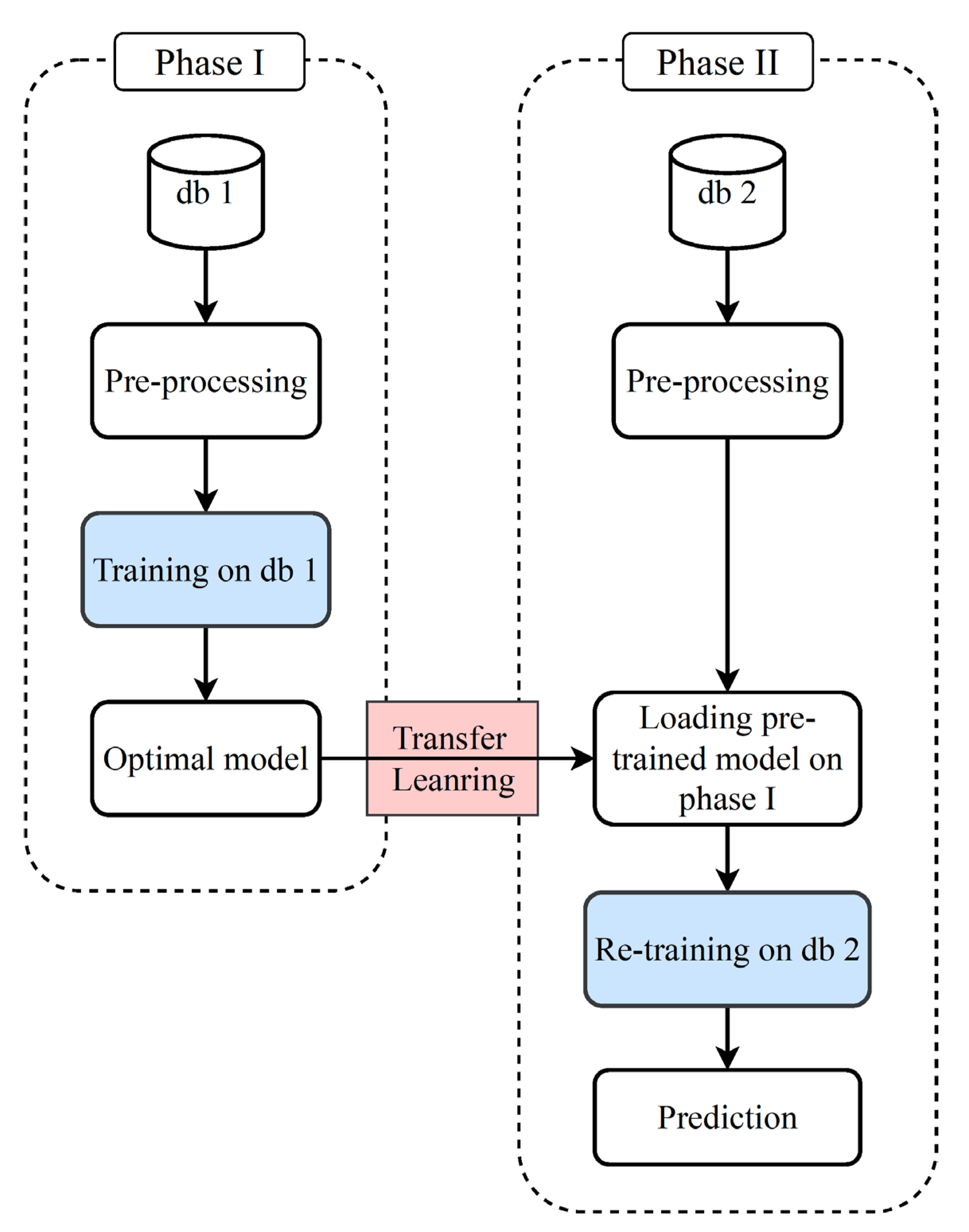
This study presents a framework, as presented in Figure 1, based on deep learning and transfer learning. This framework consists of two phases. In the first phase, the rich dataset of db 1 is used to build and train the optimal model for hourly day-ahead PV power forecasting. Then, such a model is transferred to phase II for PV power prediction on db 2. The presented framework leverages the power of deep learning and transfer learning to improve the accuracy of day-ahead PV power forecasting. The deep learning model in phase I is trained using a large and diverse dataset from db 1, allowing for the capturing of complex relationships between various meteorological variables and PV power production. The transfer learning process in phase II fine-tunes the pretrained model from phase I, utilizing the limited data from db 2, and improves its ability to perform accurate predictions for the second PV power farm. The proposed framework provides a practical solution for PV power forecasting in real-world applications, especially in cases where limited historical data are available. As presented in Table 2, these two databases have different statistical behavior; for example, the rated power of db 1 is about 75 [kW], while db 2 rated power is much higher (243 [kW]). However, as presented later, the advantage of transfer learning using neural networks prevents the trained model from working poorly on db 2. In the preprocessing step, each dataset is cleaned and normalized with the z-score formula presented in (1), considering their mean (μ) and standard deviations (σ) of input feature space (x).
x′ = (x − μ)/σ
In phase II, the achieved optimal model in phase I is loaded to be retrained by the normalized dataset of db 2. In the training step in phase II, the earlier layers of the transferred model are frozen to avoid losing the learned patterns from db 1; therefore, their weight values are not updated, and only the weight values of the last layer are updated. The test dataset of db2 is normalized by the mean and standard deviation calculated for the training dataset of db2. The outputs of models are then denormalized with these values to have the same actual scale to evaluate the accuracy and performance of the models.
3. Results and Discussion
The linear model and three state-of-the-art deep learning models—a feedforward neural network, convolutional neural network, and long short-term memory—have been trained based on the framework presented in Figure 1. The models are optimized considering MAE (mean absolute error) as a cost function (2), and Bayesian optimization is employed to select the best hyperparameters for models. Bayesian optimization, a probabilistic method for optimizing hyperparameters, ensures that the models are trained with optimal settings, resulting in improved prediction accuracy:
where is the total number in the sample. The sliding window is used to build the input–output pairs for the regression purpose of this study. Each input consists of information for five days (PV power, temperature, and time), and the associated output is a day ahead of the PV power output. In other words, a model will predict PV power production (24 samples, 1 per hour) by looking only at the historical dataset of the last five days (120 input samples for each PV power, temperature, and time per hour).
The results of these models are compared and analyzed to evaluate their performance in terms of accuracy and computational efficiency. The comparison provides a comprehensive evaluation of the proposed framework and helps to determine the most suitable model for day-ahead PV power forecasting with transfer learning. In order to evaluate the performance of models and compare their accuracy in day-ahead PV power prediction, various evaluation metrics are taken into account, such as mean square error (MSE), mean absolute percentage error (MAPE), root mean square error (RMSE), and weighted mean absolute percentage error (wMAPE), as presented in (3)–(6), respectively:
wMAPE determines the average difference between the predicted and actual values by considering the magnitude of the actual values. This metric generates a weighted average of the absolute percentage errors, with the weight determined by the size of the actual values. Hence, wMAPE is particularly apt for evaluating forecasting models in situations where the actual values display substantial fluctuations in magnitude.
3.1. Training the Base Model
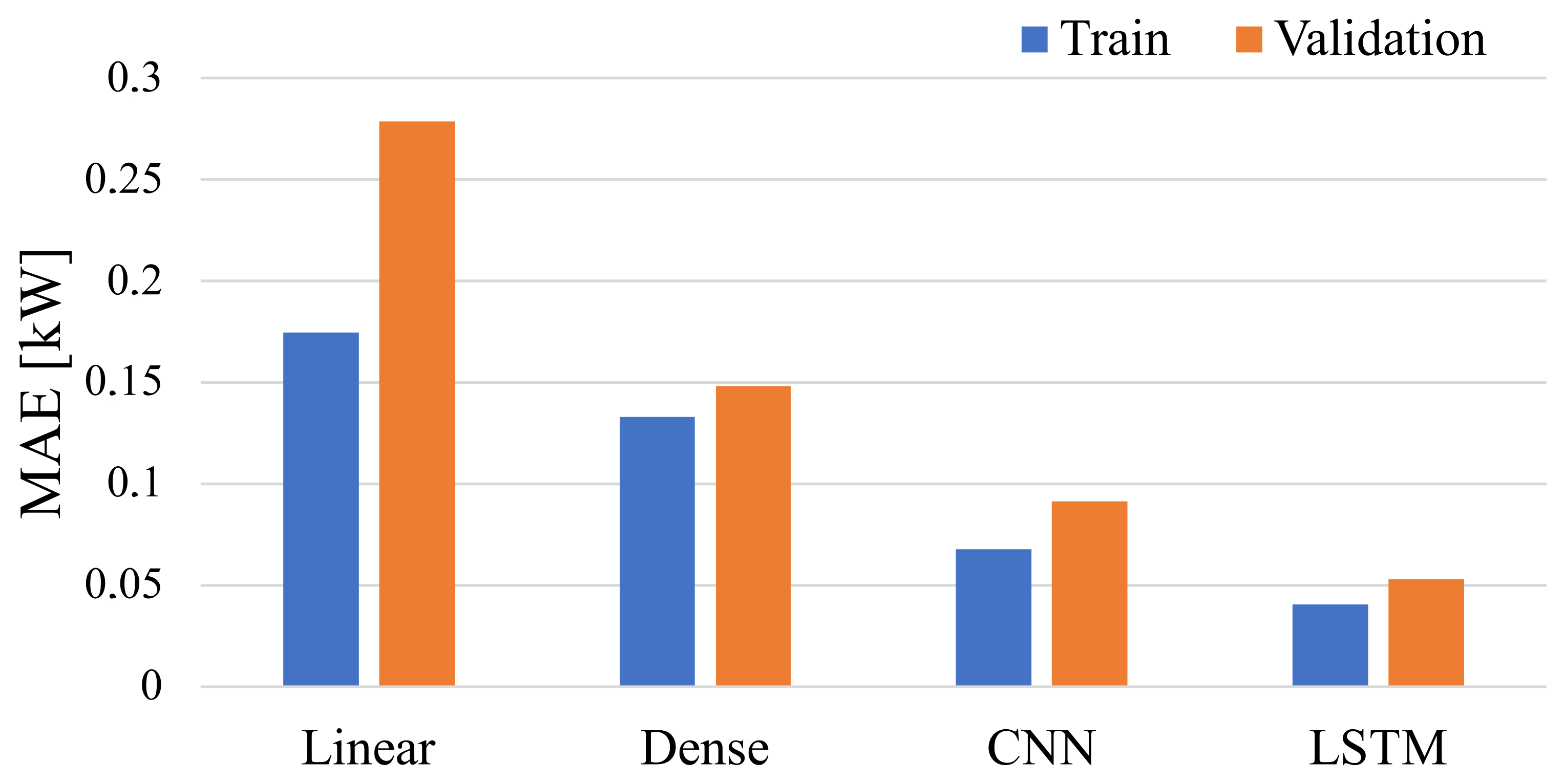
In the first modeling phase, the four models are trained using a historical dataset of db 1: 80% of the dataset is used for training and 20% for validation of the models. When there are limited data available, dividing it into only training and validation sets can provide a viable solution. This approach allows for both training the model and evaluating its performance. As shown in Figure 2, the models have good overall performance on both training and validation sets. The models based on CNN and LSTM have comparably better accuracy since their internal structure has been designed to analyze sequence data, allowing them to capture important features in the time-series dataset effectively. As expected, the LSTM model performance in capturing hidden features in a time-series dataset is superior, thanks to the various gates it has to determine which information should be forgotten, remembered, or passed to the next cell. With their promising performance, these base models will serve as the foundation for the transfer learning phase. This study presents MAE and MSE in kW units.
The accuracy of the trained models regarding different evaluation metrics is presented in Table 3. The model based on LSTM has the best accuracy in all metrics, with an MAE of 0.052, MSE of 0.015, MAPE of 24%, RMSE of 0.101, and wMAPE of 25.05%. These results show that all models have reasonable accuracy to be used in the second phase of the modeling. Additionally, the results of the accuracy evaluation demonstrate the effectiveness of the proposed framework in improving prediction performance. The outstanding performance of the LSTM model, with a low MAE, MSE, and RMSE, highlights its potential as a robust solution for day-ahead PV power forecasting. The MAPE and wMAPE, which measure the percentage of error in the predictions, further validate the results and show that the models have a high level of accuracy.
3.2. Transfer Learning
The trained models in phase I are transferred to the phase II setting in the second part of modeling. The first three months (the beginning of September 2017 to the end of December 2017) of db 2 are considered a training set, while the dataset regarding January 2018 in this database is considered for the test to evaluate the performance of the models.
This study also trains new linear, dense, CNN, and LSTM models considering the training set of db 2 to evaluate performance models transferred from phase I. The last layers of transferred models are also retrained by a training set constructed of db 2. This study investigates the implementing of transfer learning by evaluating the performance of transferred models against newly trained models. The transfer models, retrained transferred models, and new models are all evaluated on the test set of db 2 to assess their ability to generalize to new data. By comparing the results, this study provides insights into the efficacy of transfer learning and highlights the factors that impact its performance. Therefore, the following sets of models are considered:
- New model: a set of new models trained by the training set of db 2. These models are developed specifically for the data and requirements of phase II.
- Transfer: a set of models transferred from phase I that have undergone minimal modifications. These models are not retrained, but rely on their preexisting knowledge and training to perform predictions in the new environment of phase II.
- Trained transfer: a set of models transferred from phase I, but have been further trained using the training set of db 2. These models benefit from the knowledge and training acquired during phase I, but also incorporate new information and adapt to the specifics of the new environment in phase II. As a result, the performance of these models may be improved compared to the transferred models.
Figure 3 demonstrates the accuracy of these three sets of models in terms of MAE on the test set of db 2. As is shown, the new linear model has the worst performance due to a lack of enough data for training. In contrast, the transferred models have better performances, especially in the case of the linear model: the accuracy of the transferred linear model improved dramatically. This figure examines the top models by closely evaluating the results from the dense, CNN, and LSTM models. The chart clearly compares the performance of models through a detailed and concise view. Considering only nonlinear models (dense, CNN, LSTM), the new models based on CNN and LSTM work better than the dense model. At the same time, the untrained transferred CNN works better than the untrained transferred LSTM version. Generally, retraining models with the training set of db 2 enhanced the precision of models. The transferred LSTM accuracy is improved more compared to the transferred CNN. The retrained LSTM model has the best performance among all nine presented models. It is important to note that the choice of the model depends on the particular problem and the characteristics of the data. Although LSTM and CNN models may perform better in some cases, dense models may still be appropriate for simpler tasks or smaller datasets. Transfer learning can be beneficial in reducing the amount of training data needed and accelerating the training process.
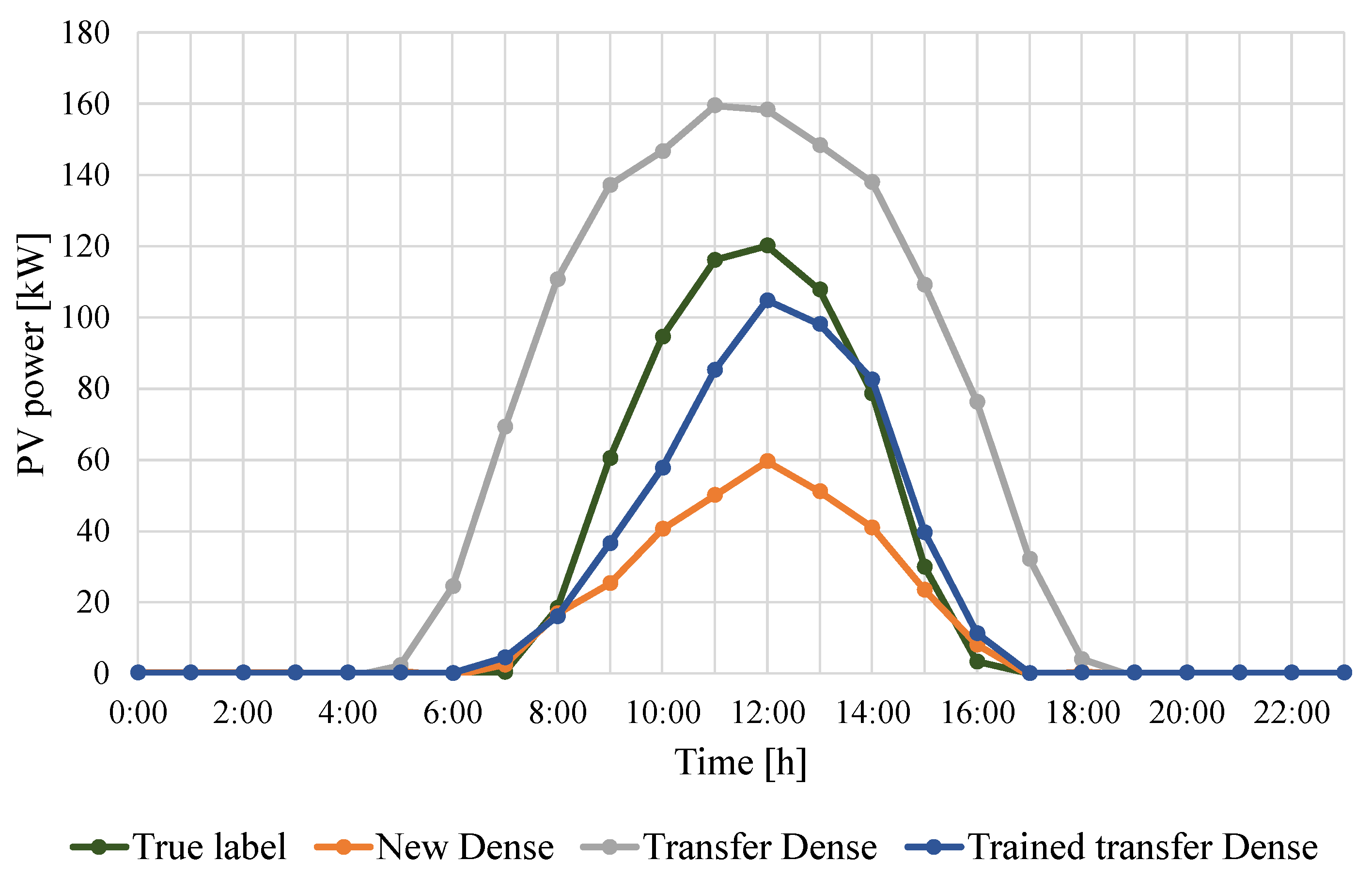
Figure 4 illustrates an hourly day-ahead PV power prediction of a random date in the test set of db 2 based on the dense model. The new dense model failed to predict the day ahead accurately due to the fact that deep learning models need a lot of data to be able to generalize with acceptable precision. Similarly, the transferred dense network, which has yet to be retrained, could not foresee this date well enough. However, retraining this network with information on db 2 improves the accuracy of the model in such a way that its prediction is closer to actual labels than the other two models presented in this figure.
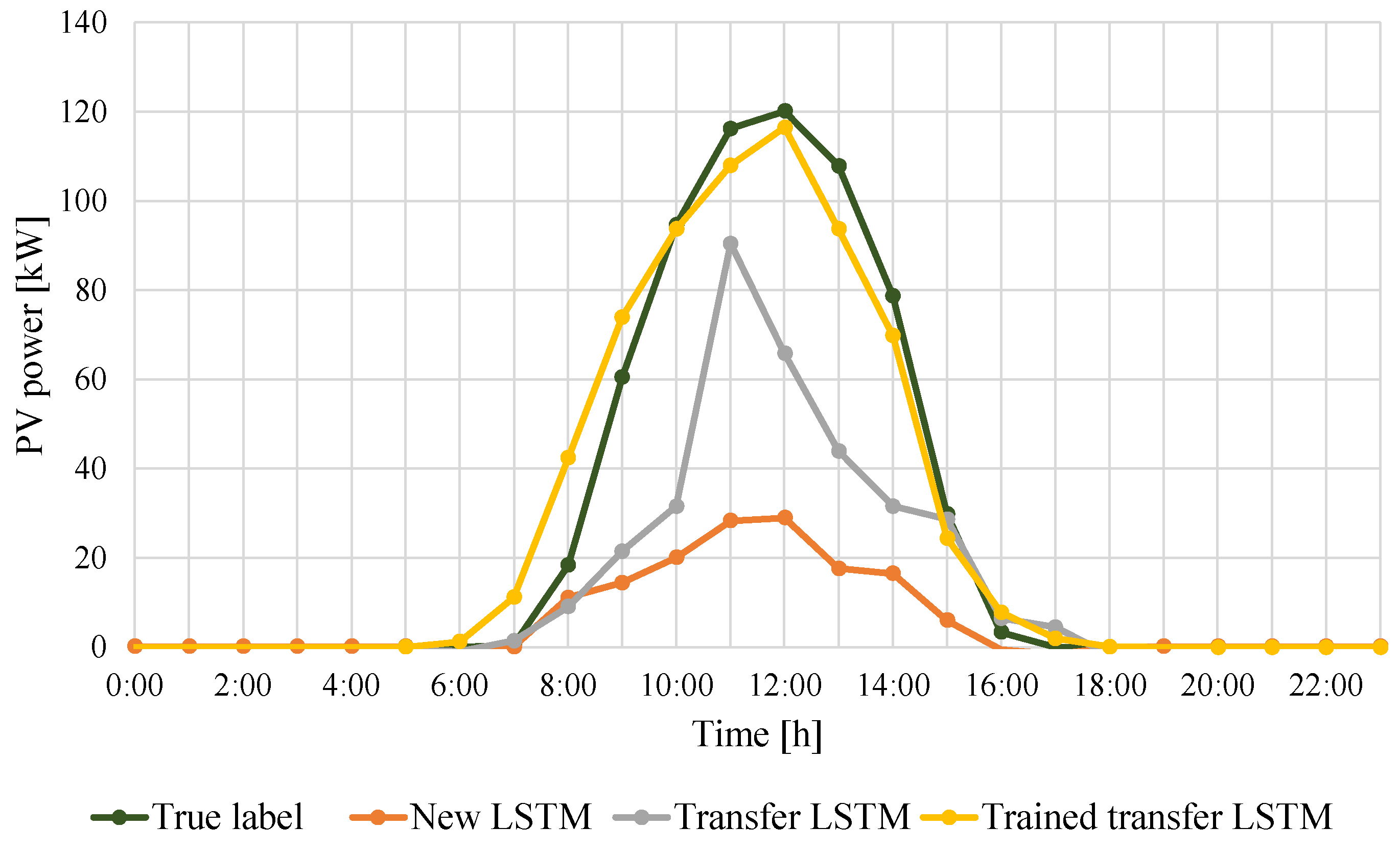
Figure 5 illustrates an hourly day-ahead PV power prediction of a random date in the test set of db 2 based on the LSTM networks. Similarly to dense networks, the new LSTM model and transferred LSTM model do not accurately predict the day ahead of the sample example. One of the reasons that untrained transferred models have poor performance is the different scales and rated power that the two datasets have. Moreover, the statistical properties and distribution of these datasets are different. Therefore, the performance of transferred models significantly improved after retraining them even with the exiguous training set of db 2.
Figure 6 illustrates an hourly day-ahead PV power prediction of a random date in the test set of db 2 based on transfer learning. All the models presented in this figure are retrained with the training set of db 2. Thus, they have superior performance compared to other groups of models, namely, new models and untrained transferred models. Above all, the trained transferred LSTM model shows the best precision, since it is designed to capture hidden patterns in sequences such as time-series datasets.
Table 4 presents the accuracy of all 12 models presented in phase II of the proposed framework. The models based on transfer learning perform superiorly in day-ahead PV power prediction compared to new models using the limited available dataset in db 2. For instance, the linear model has inferior performance, while the linear transferred version enhanced PV prediction accuracy dramatically. The models based on the LSTM network generally perform better in most evaluation metrics. However, the trained transfer CNN model works slightly better than the untrained transfer LSTM model. After training untrained transfer models, the LSTM model improves more than the CNN model in MAE, MSE, and RMSE values and has lower values for these metrics. On the other hand, CNN reaches the lowest MAPE—68.25%.
In this study, all the modeling was performed in Python programing language on a workstation with an i7-8700K CPU and 16 GB RAM. Various packages and libraries were used for data processing, neural network modeling and optimization, and visualization, including NumPy, Pandas, TensorFlow, and Matplotlib. In transfer learning, a pretrained model is fine-tuned on a new task, allowing the model to leverage its prior knowledge to solve the new problem more efficiently. This can result in improved accuracy as well as reduced training time, as demonstrated in Table 5. Table 5 presents the computational time for training neural networks in phases I and II. The time unit in this table is minutes. Since more data are available in phase I, the computational time is comparably higher than training the original model in phase II. On the other hand, implementing transfer learning improved not only the accuracy but also the training time; for example, the training time for the LSTM model was reduced from 201 to 76 min. Using a pretrained model, the model can quickly adapt to the new task, reducing the time required for training and leveraging the features learned from the previous task, leading to improved performance.
4. Conclusions
Deep learning models have achieved reliable and accurate extrapolation and prediction in solar energy prediction in recent years. However, the accuracy of these models strongly depends on the historical dataset size, and the precision of their forecasting is low if not enough data are available. Thus, this study presents a data-driven framework based on transfer learning and deep neural network to predict day-ahead PV power generation for newly installed PV power plants.
In the first phase of the framework, four predictive models based on linear, dense, CNN, and LSTM networks are trained and optimized with a rich PV system dataset. Then, these reliable models are transferred to the second phase associated with the newly installed PV power plant in the same region. New models based on previous architecture are trained with the dataset of the newly installed PV power plant. The results show that the transferred models retrained with the new dataset perform better than other models. Among all 12 models presented in this study, the retrained transferred LSTM model has the best accuracy with an MAE of 0.211, MSE of 0.168, MAPE of 74%, RMSE of 0.403, and wMAPE of 32.04%, even though the rated PV production power of two PV plants is quite different.
Author Contributions
Conceptualization, S.M.M.; methodology, S.M.M.; formal analysis, S.M.M.; investigation, S.M.M.; resources, S.M.M. and M.L.; writing—original draft preparation, S.M.M. and C.G.C.; writing—review and editing, S.M.M., C.G.C., M.L. and F.F.; visualization, S.M.M.; supervision, S.M.M. and M.L.; project administration, S.M.M. and M.L. All authors have read and agreed to the published version of the manuscript.
Funding
This research received no external funding.
Data Availability Statement
Supporting data are not available.
Acknowledgments
Not applicable.
Conflicts of Interest
The authors declare no conflict of interest.
Abbreviations
| Abbreviation | Terminology |
| PV | Photovoltaic |
| EV | Electric vehicle |
| ML | Machine learning |
| DL | Deep learning |
| RL | Reinforcement learning |
| TL | Transfer learning |
| FNN | Feedforward neural network |
| CNN | Convolutional neural network |
| LSTM | Long short-term memory |
| ReLU | Rectified linear unit |
| RNN | Recurrent neural network |
| db # | Database number |
| μ | Mean |
| σ | Standard deviations |
| x | Input feature space |
| MAE | Mean absolute error |
| Total number in the sample | |
| MSE | Mean square error |
| MAPE | Mean absolute percentage error |
| RMSE | Root mean square error |
| wMAPE | Weighted mean absolute percentage error |
References
- García-Triviño, P.; Sarrias-Mena, R.; García-Vázquez, C.A.; Leva, S.; Fernández-Ramírez, L.M. Optimal Online Battery Power Control of Grid-Connected Energy-Stored Quasi-Impedance Source Inverter with PV System. Appl. Energy 2023, 329, 120286. [Google Scholar] [CrossRef]
- Miraftabzadeh, S.M.; Longo, M.; Foiadelli, F. Estimation Model of Total Energy Consumptions of Electrical Vehicles under Different Driving Conditions. Energies 2021, 14, 854. [Google Scholar] [CrossRef]
- Dimitropoulos, N.; Sofias, N.; Kapsalis, P.; Mylona, Z.; Marinakis, V.; Primo, N.; Doukas, H. Forecasting of Short-Term PV Production in Energy Communities through Machine Learning and Deep Learning Algorithms. In Proceedings of the 2021 12th International Conference on Information, Intelligence, Systems & Applications (IISA), Chania Crete, Greece, 12–14 July 2021; pp. 1–6. [Google Scholar] [CrossRef]
- Touati, F.; Chowdhury, N.A.; Benhmed, K.; San Pedro Gonzales, A.J.R.; Al-Hitmi, M.A.; Benammar, M.; Gastli, A.; Ben-Brahim, L. Long-Term Performance Analysis and Power Prediction of PV Technology in the State of Qatar. Renew. Energy 2017, 113, 952–965. [Google Scholar] [CrossRef]
- Karabiber, A.; Alçin, Ö.F. Short Term PV Power Estimation by means of Extreme Learning Machine and Support Vector Machine. In Proceedings of the 2019 7th International Istanbul Smart Grids and Cities Congress and Fair (ICSG), Istanbul, Turkey, 25–26 April 2019; pp. 41–44. [Google Scholar] [CrossRef]
- Rana, M.; Rahman, A.; Jin, J. A Data-driven Approach for Forecasting State Level Aggregated Solar Photovoltaic Power Production. In Proceedings of the 2020 International Joint Conference on Neural Networks (IJCNN), Glasgow, UK,, 19–24 July 2020; pp. 1–8. [Google Scholar] [CrossRef]
- Khandakar, A.; Chowdhury, M.E.H.; Kazi, M.K.; Benhmed, K.; Touati, F.; Al-Hitmi, M.; Gonzales, A.S.P. Machine Learning Based Photovoltaics (PV) Power Prediction Using Different Environmental Parameters of Qatar. Energies 2019, 12, 2782. [Google Scholar] [CrossRef] [Green Version]
- Mellit, A.; Pavan, A.M.; Ogliari, E.; Leva, S.; Lughi, V. Advanced Methods for Photovoltaic Output Power Forecasting: A Review. Appl. Sci. 2020, 10, 487. [Google Scholar] [CrossRef] [Green Version]
- Miraftabzadeh, S.M.; Longo, M.; Foiadelli, F.; Pasetti, M.; Igual, R. Advances in the Application of Machine Learning Techniques for Power System Analytics: A Survey. Energies 2021, 14, 4776. [Google Scholar] [CrossRef]
- Miraftabzadeh, S.M.; Longo, M.; Foiadelli, F. A-Day-Ahead Photovoltaic Power Prediction Based on Long Short Term Memory Algorithm. In Proceedings of the SEST 2020—3rd International Conference on Smart Energy Systems and Technologies, Istanbul, Turkey, 7–9 September 2020; Institute of Electrical and Electronics Engineers Inc.: Piscataway, NJ, USA, 2020. [Google Scholar]
- Ahmed, R.; Sreeram, V.; Mishra, Y.; Arif, M.D. A Review and Evaluation of the State-of-the-Art in PV Solar Power Forecasting: Techniques and Optimization. Renew. Sustain. Energy Rev. 2020, 124, 109792. [Google Scholar] [CrossRef]
- Mohan, V.; Senthilkumar, S. IoT Based Fault Identification in Solar Photovoltaic Systems Using an Extreme Learning Machine Technique. J. Intell. Fuzzy Syst. 2022, 43, 3087–3100. [Google Scholar] [CrossRef]
- Daliento, S.; Chouder, A.; Guerriero, P.; Pavan, A.M.; Mellit, A.; Moeini, R.; Tricoli, P. Monitoring, Diagnosis, and Power Forecasting for Photovoltaic Fields: A Review. Int. J. Photoenergy 2017, 2017, 1356851. [Google Scholar] [CrossRef]
- Kong, Z.; Xia, Z.; Cui, Y.; Lv, H. Probabilistic Forecasting of Short-Term Electric Load Demand: An Integra-tion Scheme Based on Correlation Analysis and Improved Weighted Extreme Learning Machine. Appl. Sci. 2019, 9, 4215. [Google Scholar] [CrossRef] [Green Version]
- Dolara, A.; Leva, S.; Manzolini, G. Comparison of Different Physical Models for PV Power Output Prediction. Sol. Energy 2015, 119, 83–99. [Google Scholar] [CrossRef] [Green Version]
- Kaaya, I.; Ascencio-Vásquez, J. Photovoltaic Power Forecasting Methods. In Solar Radiation-Measurement, Modeling and Forecasting Techniques for Photovoltaic Solar Energy Applications; IntechOpen: London, UK, 2021. [Google Scholar]
- Zhang, Y.; Wang, J. GEFCom2014 Probabilistic Solar Power Forecasting Based on K-Nearest Neighbor and Kernel Density Estimator. In Proceedings of the IEEE Power and Energy Society General Meeting, Denver, CO, USA, 26–30 July 2015; Volume 2015. [Google Scholar]
- Das, U.K.; Tey, K.S.; Seyedmahmoudian, M.; Mekhilef, S.; Idris, M.Y.I.; van Deventer, W.; Horan, B.; Stojcevski, A. Forecasting of Photovoltaic Power Generation and Model Optimization: A Review. Renew. Sustain. Energy Rev. 2018, 81, 912–928. [Google Scholar] [CrossRef]
- Dolara, A.; Grimaccia, F.; Leva, S.; Mussetta, M.; Ogliari, E. A Physical Hybrid Artificial Neural Network for Short Term Forecasting of PV Plant Power Output. Energies 2015, 8, 1138–1153. [Google Scholar] [CrossRef] [Green Version]
- Liu, L.; Zhao, Y.; Chang, D.; Xie, J.; Ma, Z.; Sun, Q.; Yin, H.; Wennersten, R. Prediction of Short-Term PV Power Output and Uncertainty Analysis. Appl. Energy 2018, 228, 700–711. [Google Scholar] [CrossRef]
- Lee, H.Y.; Kim, N.W.; Lee, J.G.; Lee, B.T. Uncertainty-Aware Forecast Interval for Hourly PV Power Output. IET Renew. Power Gener. 2019, 13, 2656–2664. [Google Scholar] [CrossRef]
- Netsanet, S.; Zhang, J.; Zheng, D.; Agrawal, R.K.; Muchahary, F. An Aggregative Machine Learning Approach for Output Power Prediction of Wind Turbines. In Proceedings of the 2018 IEEE Texas Power and Energy Conference, TPEC 2018, College Station, TX, USA, 8–9 February 2018; pp. 1–6. [Google Scholar]
- Mohammadi, Y.; Mahdi Miraftabzadeh, S.; Bollen, M.H.J.; Longo, M. Seeking Patterns in Rms Voltage Variations at the Sub-10-Minute Scale from Multiple Locations via Unsupervised Learning and Patterns’ Post-Processing. Int. J. Electr. Power Energy Syst. 2022, 143, b108516. [Google Scholar] [CrossRef]
- Khodayar, M.; Liu, G.; Wang, J.; Khodayar, M.E. Deep Learning in Power Systems Research: A Review. CSEE J. Power Energy Syst. 2021, 7, 209–220. [Google Scholar]
- Ozcanli, A.K.; Yaprakdal, F.; Baysal, M. Deep Learning Methods and Applications for Electrical Power Sys-tems: A Comprehensive Review. Int. J. Energy Res. 2020, 44, 7136–7157. [Google Scholar] [CrossRef]
- Miraftabzadeh, S.M.; Foiadelli, F.; Longo, M.; Pasetti, M. A Survey of Machine Learning Applications for Power System Analytics. In Proceedings of the 2019 IEEE International Conference on Environment and Electrical Engineering and 2019 IEEE Industrial and Commercial Power Systems Europe (EEEIC/I CPS Europe), Genova, Italy, 11–14 June 2019; pp. 1–5. [Google Scholar]
- Mohammadi, Y.; Miraftabzadeh, S.M.; Bollen, M.H.J.; Longo, M. Voltage-Sag Source Detection: Developing Supervised Methods and Proposing a New Unsupervised Learning. Sustain. Energy Grids Netw. 2022, 32, 100855. [Google Scholar] [CrossRef]
- Miraftabzadeh, S.M.; Longo, M.; Brenna, M.; Pasetti, M. Data-Driven Model for PV Power Generation Patterns Extraction via Unsupervised Machine Learning Methods. In Proceedings of the 2022 North American Power Symposium (NAPS), Salt Lake City, UT, USA, 9–11 October 2022; pp. 1–5. [Google Scholar]
- Mishra, M.; Nayak, J.; Naik, B.; Abraham, A. Deep Learning in Electrical Utility Industry: A Comprehensive Review of a Decade of Research. Eng. Appl. Artif. Intell. 2020, 96, 104000. [Google Scholar] [CrossRef]
- Li, B.; Delpha, C.; Diallo, D.; Migan-Dubois, A. Application of Artificial Neural Networks to Photovoltaic Fault Detection and Diagnosis: A Review. Renew. Sustain. Energy Rev. 2021, 138, 110512. [Google Scholar] [CrossRef]
- Mohammadi, Y.; Miraftabzadeh, S.M.; Bollen, M.H.J.; Longo, M. An Unsupervised Learning Schema for Seeking Patterns in Rms Voltage Variations at the Sub-10-Minute Time Scale. Sustain. Energy Grids Netw. 2022, 31, 100773. [Google Scholar] [CrossRef]
- Berghout, T.; Benbouzid, M.; Bentrcia, T.; Ma, X.; Djurović, S.; Mouss, L.H. Machine Learning-Based Condi-tion Monitoring for Pv Systems: State of the Art and Future Prospects. Energies 2021, 14, 6316. [Google Scholar] [CrossRef]
- Aldhshan, S.R.S.; Abdul Maulud, K.N.; Wan Mohd Jaafar, W.S.; Karim, O.A.; Pradhan, B. Energy Consumption and Spatial Assessment of Renewable Energy Penetration and Building Energy Efficiency in Malaysia: A Review. Sustainability 2021, 13, 9244. [Google Scholar] [CrossRef]
- Aziz, F.; Ul Haq, A.; Ahmad, S.; Mahmoud, Y.; Jalal, M.; Ali, U. A Novel Convolutional Neural Network-Based Approach for Fault Classification in Photovoltaic Arrays. IEEE Access 2020, 8, 41889–41904. [Google Scholar] [CrossRef]
- Cheng, L.; Zang, H.; Ding, T.; Wei, Z.; Sun, G. Multi-Meteorological-Factor-Based Graph Modeling for Photovoltaic Power Forecasting. IEEE Trans. Sustain. Energy 2021, 12, 1593–1603. [Google Scholar] [CrossRef]
- Wen, S.; Zhang, C.; Lan, H.; Xu, Y.; Tang, Y.; Huang, Y. A Hybrid Ensemble Model for Interval Prediction of Solar Power Output in Ship Onboard Power Systems. IEEE Trans. Sustain. Energy 2021, 12, 14–24. [Google Scholar] [CrossRef]
- Abubakar Mas’ud, A. Comparison of Three Machine Learning Models for the Prediction of Hourly PV Out-put Power in Saudi Arabia. Ain Shams Eng. J. 2022, 13, 101648. [Google Scholar] [CrossRef]
- Benhmed, K.; Touati, F.; Al-Hitmi, M.; Chowdhury, N.A.; Gonzales, A.S.P.; Qiblawey, Y.; Benammar, M. PV Power Prediction in Qatar Based on Machine Learning Approach. In Proceedings of the 2018 6th International Renewable and Sustainable Energy Conference, IRSEC 2018, Rabat, Morocco, 5–8 December 2018. [Google Scholar]
- Cecaj, A.; Lippi, M.; Mamei, M.; Zambonelli, F. Sensing and Forecasting Crowd Distribution in Smart Cities: Potentials and Approaches. IoT 2021, 2, 33–49. [Google Scholar] [CrossRef]
- Zhao, J.; Yu, H.; Geng, G. TransOS-ELM: A Short-Term Photovoltaic Power Forecasting Method Based on Transferred Knowledge from Similar Days. In Proceedings of the 5th IEEE Conference on Energy Internet and Energy System Integration: Energy Internet for Carbon Neutrality, EI2 2021, Taiyuan, China, 22–24 October 2021; pp. 89–94. [Google Scholar]
- Jung, S.M.; Park, S.; Jung, S.W.; Hwang, E. Monthly Electric Load Forecasting Using Transfer Learning for Smart Cities. Sustainability 2020, 12, 6364. [Google Scholar] [CrossRef]
- Yu, F.; Xiu, X.; Li, Y. A Survey on Deep Transfer Learning and Beyond. Mathematics 2022, 10, 3619. [Google Scholar] [CrossRef]
- Akram, M.W.; Li, G.; Jin, Y.; Chen, X.; Zhu, C.; Ahmad, A. Automatic Detection of Photovoltaic Module De-fects in Infrared Images with Isolated and Develop-Model Transfer Deep Learning. Sol. Energy 2020, 198, 175–186. [Google Scholar] [CrossRef]
- Zhou, S.; Zhou, L.; Mao, M.; Xi, X. Transfer Learning for Photovoltaic Power Forecasting with Long Short-Term Memory Neural Network. In Proceedings of the 2020 IEEE International Confer-ence on Big Data and Smart Computing, BigComp 2020, Busan, Republic of Korea, 19–22 February 2020; pp. 125–132. [Google Scholar]
Figure 1.
The presented framework of a-day-ahead PV power prediction using transfer learning and deep neural network.
Figure 1.
The presented framework of a-day-ahead PV power prediction using transfer learning and deep neural network.

Figure 2.
The performance of linear, dense, CNN, and LSTM learning models on the first database in terms of MAE (kW).
Figure 2.
The performance of linear, dense, CNN, and LSTM learning models on the first database in terms of MAE (kW).

Figure 3.
The accuracy of the three sets of models presented in terms of MAE [kW] on the test set of db 2. To thoroughly evaluate the top-performing models, this figure focuses on a close examination of the results obtained from the dense, CNN, and LSTM models. The zoomed-in chart offers a clear and concise comparison of the performance of each model.

Figure 4.
Day-ahead prediction of the PV power output of a random date in the test set for models based on the dense network.
Figure 4.
Day-ahead prediction of the PV power output of a random date in the test set for models based on the dense network.

Figure 5.
Day-ahead prediction of the PV power output of a random date in the test set for models based on the LSTM network.
Figure 5.
Day-ahead prediction of the PV power output of a random date in the test set for models based on the LSTM network.

Figure 6.
Day-ahead prediction of the PV power output of a random date in the test set for models based on the transfer learning.
Figure 6.
Day-ahead prediction of the PV power output of a random date in the test set for models based on the transfer learning.


Table 1.
Forecasting type, method, and utility based on the different approaches for predictions [8,11,14,18,19,20,21].
| Approach Type | Forecasting Type | Method | Utility |
|---|---|---|---|
| Phenomenological approach | Medium/long-term forecasting | Numerical weather prediction, satellite images for regional models. | Maintenance and PV plant planning. |
| Statistical approach | Short-term forecasting up to one day ahead | Include regression models, exponential smoothing, autoregressive models, autoregressive moving integrated average, time series ensemble, and probabilistic approaches. | Control of power system operation, unit commitment, and sales. |
| ML approach | From short-term forecasting up to the long-term horizon | Cross-sectoral method, which combines models and Artificial Intelligence. | Production, anomaly detection, and energy disaggregation. |
| Hybrid approach | From short-term forecasting up to the long-term horizon | Combine one of the mentioned advanced methods with one physical or statistical approach. | From short-term power production to maintenance and plant planning. |
| Probabilistic approach | From short-term forecasting up to medium-term horizon | Provide output with quantile, interval and density function. | Electric load forecasting |
Table 2.
Dataset description used in this study.
| Database | Rated Power [kW] | Duration | Average of Power [kW] | Standard Deviation of Power | Location * [] |
|---|---|---|---|---|---|
| db 1 | 75 | 2015 (January)–2017 (December) | 10.05 | 16.44 | [39.1385, −77.2155] |
| db 2 | 243 | 2017 (September)–2018 (January) | 33.14 | 52.94 | [39.1319, −77.2041] |
* Location in this table is presented in latitude and longitude pairs.
Table 3.
The performances of presented models on db 1 considering different evaluation metrics.
| Model | MAE * | MSE * | MAPE | RMSE | wMAPE |
|---|---|---|---|---|---|
| Linear | 0.278 | 0.118 | 98.90 | 0.344 | 73.61 |
| Dense | 0.148 | 0.066 | 64.17 | 0.258 | 43.15 |
| CNN | 0.091 | 0.045 | 45.31 | 0.212 | 39.59 |
| LSTM | 0.052 | 0.015 | 24.00 | 0.101 | 25.05 |
* MAE and MSE in kW.
Table 4.
The performance of presented models on db 2 by considering different evaluation metrics.
| Model | MAE * | MSE * | MAPE | RMSE | wMAPE | |
|---|---|---|---|---|---|---|
| Linear | New | 7.122 | 176.42 | 5775.01 | 12.05 | 640.93 |
| Untrained transfer | 0.685 | 1.81 | 293.22 | 1.345 | 150.92 | |
| Trained transfer | 0.572 | 1.538 | 252.58 | 1.146 | 120.34 | |
| Dense | New | 1.044 | 2.67 | 466.67 | 1.636 | 170.76 |
| Untrained transfer | 0.390 | 0.346 | 268.22 | 0.589 | 98.69 | |
| Trained transfer | 0.236 | 0.246 | 198.39 | 0.496 | 33.97 | |
| CNN | New | 0.360 | 0.462 | 165.56 | 0.68 | 41.97 |
| Untrained transfer | 0.253 | 0.268 | 145.17 | 0.501 | 36.25 | |
| Trained transfer | 0.231 | 0.197 | 68.25 | 0.437 | 34.98 | |
| LSTM | New | 0.3615 | 0.55 | 109.99 | 0.745 | 47.07 |
| Untrained transfer | 0.313 | 0.387 | 97.20 | 0.622 | 45.07 | |
| Trained transfer | 0.211 | 0.168 | 74.44 | 0.403 | 32.04 | |
* MAE and MSE are in kW.
Table 5.
The computational time for training neural networks in phase I and II of modeling.
| Model | Phase I | Phase II | |
|---|---|---|---|
| Original | Transfer | ||
| Dense | 175 * | 44 | 23 |
| CNN | 375 | 150 | 38 |
| LSTM | 750 | 201 | 76 |
* Computational times in this table presented in minutes.
Disclaimer/Publisher’s Note: The statements, opinions and data contained in all publications are solely those of the individual author(s) and contributor(s) and not of MDPI and/or the editor(s). MDPI and/or the editor(s) disclaim responsibility for any injury to people or property resulting from any ideas, methods, instructions or products referred to in the content. |
© 2023 by the authors. Licensee MDPI, Basel, Switzerland. This article is an open access article distributed under the terms and conditions of the Creative Commons Attribution (CC BY) license (https://creativecommons.org/licenses/by/4.0/).
Share and Cite
MDPI and ACS Style
Miraftabzadeh, S.M.; Colombo, C.G.; Longo, M.; Foiadelli, F. A Day-Ahead Photovoltaic Power Prediction via Transfer Learning and Deep Neural Networks. Forecasting 2023, 5, 213-228. https://doi.org/10.3390/forecast5010012
AMA Style
Miraftabzadeh SM, Colombo CG, Longo M, Foiadelli F. A Day-Ahead Photovoltaic Power Prediction via Transfer Learning and Deep Neural Networks. Forecasting. 2023; 5(1):213-228. https://doi.org/10.3390/forecast5010012
Chicago/Turabian StyleMiraftabzadeh, Seyed Mahdi, Cristian Giovanni Colombo, Michela Longo, and Federica Foiadelli. 2023. "A Day-Ahead Photovoltaic Power Prediction via Transfer Learning and Deep Neural Networks" Forecasting 5, no. 1: 213-228. https://doi.org/10.3390/forecast5010012