Article

On Forecasting Cryptocurrency Prices: A Comparison of Machine Learning, Deep Learning, and Ensembles

1
School of Computer Science & IT, University College Cork, T12 XF62 Cork, Ireland
2
Centre for Research Training in Artificial Intelligence, University College Cork, T12 XF62 Cork, Ireland
3
Insight Centre for Data Analytics, University College Cork, T12 XF62 Cork, Ireland
*
Author to whom correspondence should be addressed.
Forecasting 2023, 5(1), 196-209; https://doi.org/10.3390/forecast5010010
Submission received: 5 December 2022 / Revised: 13 January 2023 / Accepted: 18 January 2023 / Published: 29 January 2023

Abstract

:
Traders and investors are interested in accurately predicting cryptocurrency prices to increase returns and minimize risk. However, due to their uncertainty, volatility, and dynamism, forecasting crypto prices is a challenging time series analysis task. Researchers have proposed predictors based on statistical, machine learning (ML), and deep learning (DL) approaches, but the literature is limited. Indeed, it is narrow because it focuses on predicting only the prices of the few most famous cryptos. In addition, it is scattered because it compares different models on different cryptos inconsistently, and it lacks generality because solutions are overly complex and hard to reproduce in practice. The main goal of this paper is to provide a comparison framework that overcomes these limitations. We use this framework to run extensive experiments where we compare the performances of widely used statistical, ML, and DL approaches in the literature for predicting the price of five popular cryptocurrencies, i.e., XRP, Bitcoin (BTC), Litecoin (LTC), Ethereum (ETH), and Monero (XMR). To the best of our knowledge, we are also the first to propose using the temporal fusion transformer (TFT) on this task. Moreover, we extend our investigation to hybrid models and ensembles to assess whether combining single models boosts prediction accuracy. Our evaluation shows that DL approaches are the best predictors, particularly the LSTM, and this is consistently true across all the cryptos examined. LSTM reaches an average RMSE of 0.0222 and MAE of 0.0173 , respectively, 2.7 % and 1.7 % better than the second-best model. To ensure reproducibility and stimulate future research contribution, we share the dataset and the code of the experiments.

1. Introduction

Cryptocurrencies are virtual currencies that rely on blockchain technology. They have seen widespread market adoption since the introduction of Bitcoin in 2009, the most popular crypto so far. Many different subjects trade cryptos and invest in crypto funds and companies; according to CoinMarketCap [1], the global market capitalisation of cryptocurrencies reached an estimated value of USD 932.49 billion in September 2022. Although investments have seen lucrative returns, ubiquitous price fluctuations across most cryptocurrencies make such investments challenging and risky. For example, Bitcoin’s price has been highly volatile since its market launch, reaching peaks as high as +122% and +1360% in 2016 and 2017, respectively [2]. Ethereum, XRP, and Litecoin have seen similar fluctuations in 2017 alone [2].
For these reasons, investors require a forecasting approach to effectively capture crypto price fluctuations to minimise the risk and increase their profit. Moreover, it is possible to use volatility forecasts to estimate swings in their price, which is useful for developing and analysing quantitative financial trading strategies [3]. However, similar to stock price forecasting, whose market is dynamic and complex as well [4], crypto price forecasting is regarded as one of the most challenging prediction tasks in the financial domain at present [5]. Most successful researchers cast this problem as an example of time series forecasting [6,7,8,9,10,11], since the idea is to leverage historical and current price data to predict future prices over a period of time or a specific point in the future. Time series analysis has also been applied in weather forecasting and demand forecasting for retail and procurement, for example.
In the literature, the application of statistical techniques is the traditional approach for time series forecasting. Such techniques adopt statistical formulas and theories to model and capture patterns in the time series. The most frequently employed statistical models are the autoregressive integrated moving average (ARIMA) model and its variants, exponential mmoothing, multivariate linear regression, multivariate vector autoregressive model, and extended vector autoregressive model [12]. In addition, in forecasting the future prices of cryptos, the most popular example is the ARIMA [13]. Researchers have commonly employed this model to forecast Bitcoin prices [6,14,15]. Other models have also been applied, such as generalized autoregressive conditional heteroscedasticity (GARCH) models in volatility forecasting of cryptos [16,17] and diffusion processes in probabilistic forecasting of cryptos [18].
Another research branch employs machine learning (ML) models such as stochastic gradient boosting machines [19], linear regression, random forest, support vector machines, and k-nearest neighbours [20]. By leveraging historical data, these techniques focus on identifying the most influential features that determine future crypto prices to boost prediction accuracy.
A third body of work employs deep learning (DL) models to tackle crypto price forecasting, following their recent widespread success in quantitative finance [21]. Neural networks, recurrent neural networks (RNN) such as gated recurrent unit (GRU) and long short-term memory (LSTM), yemporal convolutional networks (TCN), and hybrid architectures have been applied to predict prices of Bitcoin, Ethereum, and Litecoin, for example [7,9,11]. DL approaches are considered effective at time series forecasting because they are robust to noise, they can provide native support for data sequences, and they can learn non-linear temporal dependencies on such sequences [22].
Although the literature has proposed statistical, ML, and DL techniques, there is no clear evidence of which of these approaches is superior. Indeed, the research is scattered and lacks generality because it focuses on predicting the price of a single crypto among a small number of the most popular cryptocurrencies (mainly Bitcoin). Moreover, the over-complexity of the model architecture makes their adoption in a real-world scenario very challenging because implementation, training, and predictions are expensive. Lastly, with different datasets, pre-processing strategies, and experimental methodologies, the approaches’ comparisons are inconsistent, the experiments are hard to reproduce, and their findings are therefore unreliable.
The main goal of this paper is to overcome these limitations and shed light on the effectiveness of the most popular approaches proposed in the literature so far on the crypto price prediction task. Therefore, as a major contribution, we design a framework for comparing widely used statistical, ML, and DL approaches in predicting the price of five popular cryptocurrencies, i.e., Ripple (XRP), Bitcoin (BTC), Litecoin (LTC), Ethereum (ETH), and Monero (XMR). DL networks selected include different architectures such as convolutional neural networks, recurrent neural networks, and transformers. To the best of our knowledge, we are also the first to propose using temporal fusion transformer (TFT) as a DL approach to tackle crypto price prediction. In addition, we investigate the use of hybrid models and ensembles to determine whether a combination of multiple models can improve the accuracy of the predictions.
To overcome cryptocurrency prices’ high fluctuation and volatility, we transform non-stationary time series into stationary ones by applying detrending. Predictive models are trained and tested on a 5-year time-window dataset we collected from online cryptocurrency trading platforms. Our evaluation methodology spans over one year of data and is incremental with monthly time windows. Results show that DL approaches are better than ML and statistical approaches, and, for DL models, complex architectures outperform less complex ones. To ensure reproducibility and stimulate future research contribution, we open source the dataset and the code of the experiments (https://github.com/katemurraay/tsa_crt, accessed 15 January 2023), as we believe our work to be an essential starting point for practitioners to investigate crypto price prediction.
The remainder of this paper is structured as follows: Section 2 presents the models comparison, the data collection and preprocessing, and finally describes the experimental methodology; Section 3 and Section 4 outline the results of the experiments and discuss their findings, respectively; finally, Section 5 draws conclusions and illustrates future plans.

2. Materials and Methods

In our framework, we assume the availability of a dataset of size m with daily interval granularity, i.e., each dataset’s instance refers to a timestamp day t i , i ( 1 , m ) , where t 1 and t m denote the earliest and the latest data points available in the dataset, respectively. We denote with y t i the value of the target variable at timestamp t i , i.e., the cryptocurrency price to predict. We also denote with x t i the features available at time t i ; x t i = [ y t i l , , y t i 1 ] , where l is the length of the window considered as input by the models. Our goal is to build predictive models that learn a function f ( x t i ) = y t i , see Section 2.1 for the list of models we employ in this study. This learning task is a typical example of univariate time series analysis because only one variable (i.e., the crypto price, y) varies over time.
In the remainder of this section, we describe the predictive models, the data acquisition and its preprocessing, and the experimental methodology we use to compare the models.

2.1. Predictive Models

Below we give details of the statistical, ML, DL, hybrid, and ensemble models we compare.
  • Auto Regressive Integrated Moving Average (ARIMA). This is a generalisation of the simpler ARMA model (auto regressive moving average). The traditional three-step process of constructing ARIMA models by [13], includes model identification, parameter estimation, and finally, the diagnosis of the simulation and its verification. Essentially, a prediction for a y t t a r g e t value is the linear combination of the y t i values up to the t t a r g e t timestamp and the prediction errors made for the same y x t i values. Examples of ARIMA usage include forecasting for air transport demand [23,24], long-term earning prediction [25], and next-day electricity price prediction [26]. ARIMA has effectively predicted BTC prices in [6,14,27].
  • k-Nearest Neighbor (kNN). Originally suited for classification tasks, kNN is a non-parametric model that has been successfully extended and employed for regression tasks in time series analysis. To predict y t t a r g e t , the kNN calculates the k most-similar x t i values to x t t a r g e t . Then, prediction of y t a r g e t is the weighted average of the k y t i values. The kNN model has been used in financial forecasting [28], electric market price prediction [29], and in the prediction of Bitcoin [30].
  • Support Vector Regression (SVR). Built on support vector machines for classification, SVR enables both linear and non-linear regression. Similarly to kNN, SVR is a non-parametric methodology introduced by [31]. SVR aims to maximise generalisation performance when designing regression functions [32]. SVR was applied to a variety of time series tasks such as forecasting warranty claims [32], predicting blood glucose levels [33], and for stock predictions in the financial market [34]. Examples of SVR usage in forecasting crypto prices can be found in [20,21].
  • Random Forest (RF) Regressor. This is essentially an ensemble of decision trees, each of which is built on a random subset of the training set. RF’s predictions are performed by averaging the predictions of individual trees. The key benefits of RF are its generalisation capability, and minimal sensitivity to hyperparameters [35]. RF has been used in time series tasks for forecasting cyber security incidents [36], for the prediction of methane outbreaks in coal mines usage [37], and for projecting monthly temperature variations [35]. In the prediction of cryptos, RF has been used for BTC forecasting in [20] and BTC, ETH, and XRP in [19].
  • Long Short Term Memory (LSTM). This is a type of RNN capable of learning long-term dependencies and, therefore, is suitable for time series analysis [38]. Although LSTMs follow a chain-like structure similar to ordinary RNNs, in an LSTM’s repeating module, four neural layers interact, i.e., two in the input gate, one in the forget gate, and one in the output gate. The input gate adds or updates new information, and the forget gate removes irrelevant information. The output gate ultimately passes updated information to the following LSTM cell. Examples of LSTM usage can be found in short-term travel speed prediction [39], predicting healthcare trajectories from medical records [40], and forecasting aquifer levels [41]. The model has also been successful for crypto price prediction [7,8,9].
  • Gated Recurrent Unit (GRU). Although the GRU model is similar to LSTM, the former improves upon the computational efficiency of the latter because it has fewer external gating signals in the interpolation. Consequently, the related parameters are reduced. GRU has been used in the short-term prediction for a bike-sharing service [42], network traffic predictions [43], and forecasting airborne particle pollution [44]. GRU was found in [10] to forecast the prices of BTC, ETH, and LTC successfully.
  • LSTM-GRU (HYBRID). This method was proposed by Patel et al. [11] to avail of the advantages of both LSTM and GRU. Their study indicated that this hybrid approach effectively predicted Litecoin and Monero daily prices, for this reason we include it herein. Combinations of LSTM and GRU have been successfully applied to predict water prices [45].
  • Temporal Convolution Network (TCN). Presented by Bai, Kolter, and Koltun [46], TCN is a variant of the convolutional neural network architecture, and uses dilated, causal, one-dimensional convolutional layers. TCN’s causal convolutions prevent future data from leaking into the input. TCNs have been widely adopted in time series forecasting. For example, TCNs can produce a short-term prediction of wind power [47], predict just-in-time design smells [48], and forecast in stock volatility [49]. In addition, TCN was effective at forecasting weekly Ethereum prices [50].
  • Temporal Fusion Transformer (TFT). Introduced by [51], the architecture of TFT is built on the vanilla transformer architecture. TFT is one of the most recent deep learning approaches for time series forecasting. Its design incorporates novel components such as gating mechanisms, variable section networks, static covariates, prediction intervals, and temporal processing. TFT has been applied in other time series tasks such as the prediction of pH levels in bodies of water [52], flight demand forecasting [53], and projecting future precipitation levels [54]. To the best of our knowledge, we are the first to employ it for the crypto price prediction.
We employ the voting regressor for the ensemble, a combination of different base inducers using the models described above. We build a total of 502 ensembles, one for each possible combination. An ensemble’s prediction is given by averaging the predictions from the individual models that compose the ensemble. Note that each individual model was trained separately and independently.
In our comparison, other approaches for time series forecasting could have been investigated, for example, functional data analysis for predicting electricity prices [55,56], group method of data handling and adaptive neuro-fuzzy inference system for predicting faults [57], and multi-modality graph neural network for financial time series prediction [58]. However, we limited our choice to the most popular and representative models proposed in each category (i.e., statistical, ML, and DL) in the literature because a complete and exhaustive comparison of time series methods is beyond the scope of this paper.

2.2. Data Collection

The data were gathered from Binance.com (https://www.binance.com/en, accessed 13 July 2022) and Investing.com (https://www.investing.com, accessed 13 July 2022) websites. Binance.com is the world’s largest and most popular cryptocurrency exchange portal for daily trading. It provides an array of features specific to cryptocurrency products which include market information for thousands of cryptocurrencies. Investing.com acts as a global portal for stock market information and analysis on many worldwide financial markets. For our investigation, we selected five popular cryptocurrencies in the literature, i.e., XRP, Bitcoin (BTC), Litecoin (LTC), Ethereum (ETH), and Monero (XMR).
The data collection process made use of the Binance API as a primary resource and it was complemented by information retrieved from Investing.com when missing values occurred (e.g., when the closing price of XMR was not available for a specific day). The time frame of the collected data ranges from 1 June 2017 to 31 May 2022, i.e., five years. A summary of the resulting datasets are reported in Table 1, and the covariates available for the i-th instance of each dataset are the following:
  • t i —the timestamp of the day;
  • O P t i —the opening price of the cryptocurrency at t i ;
  • H P t i —the highest price of the cryptocurrency at t i ;
  • L P t i —the lowest price of the cryptocurrency at t i ;
  • y t i —the target variable, i.e., the closing price of the cryptocurrency at t i (which corresponds to the opening price of the following day, i.e., O P t i + 1 = y t i ).
In this paper, we address the crypto price prediction task as a univariate time series analysis problem, and therefore we ignore the covariates O P , H P , and L P , but they are included in the available preprocessed dataset. We plan to consider such covariates in future work.

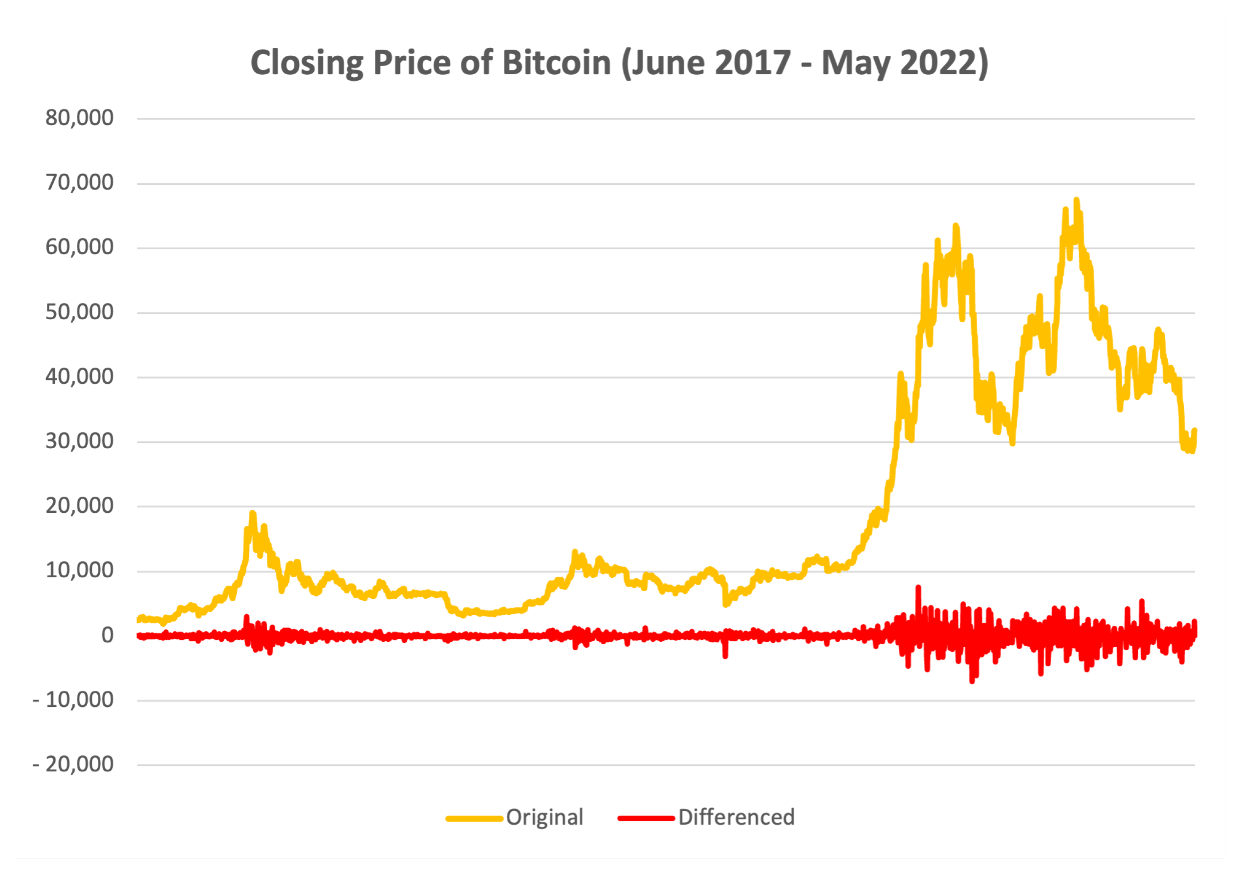
2.3. Data Pre-Processing

When forecasting with time series, their stationarity property is crucial for effective modeling [5]. A time series with mean and variance that do not change over time is referred to as stationary. On the contrary, a time series whose mean, frequency, and variance fluctuate over time and frequently display high volatility, trend, and heteroskedasticity is referred to as non-stationary [5]. Typically, traditional statistical forecasting methods such as ARIMA require time series to be stationary in order to successfully capture their properties [59]; similarly, stationarity favours learning in non-statistical models such as the ML and DL employed in this paper [60]. For these reasons, we run the augmented Dickey–Fuller (ADF) statistical test [61] to identify whether our datasets are stationary. The results show that all datasets are non-stationary except the XRP dataset.
We transform our datasets into stationary datasets by applying detrending, i.e., the process of removing the trend from a time series. In particular, we apply the differencing transformation, the simplest detrending technique that generates a new time series where the new value y t i at timestamp t i is calculated as the difference between the original observation and the observation y t i 1 at the previous time step, i.e.,
y t i = y t i y t i 1
Figure 1 shows the original Bitcoin time series in yellow and its differenced version in red. The ADF test computed on the detrended datasets confirm their stationarity.
Another typical pre-processing step that is widely adopted to enhance learning is data normalisation (e.g., [11]). We apply the Min-Max normalisation to all y t i of each dataset, so that values are mapped in the ( 0 , 1 ) range according to the following formula:
y t i = y t i y m i n y m a x y m i n
where y m i n = m i n { y t i } and y m a x = m a x { y t i } . To avoid leakage, y m i n and y m a x values are calculated from training data only.

2.4. Experimental Methodology

We performed experiments on each dataset/crypto separately, with the following methodology that was the same for all models. We performed an initial temporal training-test split on each dataset. The first 80% of the data belonged to the training set (i.e., four years of data, from t = 1 June 2017 to t = 31 May 2021 ) and the last 20% of the data belonged to the test set (i.e., one year of data, from t = 1 June 2021 to t = 31 May 2022 ). We further partitioned the test set into twelve non-overlapping monthly windows (from June 2021 to May 2022 included) and we labelled them with M i , i { 1 , 2 , , 12 } .
Inspired by [62], an incremental monthly-based strategy was employed to evaluate each model. In the first evaluation step, we trained the model on the training set, we performed predictions, and we computed the test metrics (presented in Section 2.5) on M 1 . In the second evaluation step, we included M 1 ’s data in the training set and we retrained the model from scratch on this newly enlarged training set. We again performed predictions and we computed the test metrics on M 2 . We repeated the same process for the remaining ten partitions, each time increasing the training set and moving the evaluation window one step forward. Both ML and DL models have hyperparameters; therefore, we tuned them only in the first evaluation step by using 20% of the training data for validation (optimizing for MSE), and we kept them fixed for the remainder of the evaluation. Hyperparameter details and values spaces are reported in Appendix A Table A1. We considered a sliding window of 30 days of data as input to compute a one-step-ahead prediction. To avoid overfitting of the DL models during training, we applied early stopping and we performed the experiments three times (averaging the results) to account for the randomness in the initialisation of the models.

2.5. Evaluation Metrics

To assess the quality of a model’s predictions, we computed the root mean squared error (RMSE), mean absolute error (MAE), mean absolute percentage error (MAPE), and R-squared score ( R 2 ) in each evaluation step described in the previous section, as follows:
RMSE = i = 1 n ( y t i y ^ t i ) 2 n
MAE = 1 n i = 1 n | y t i y ^ t i |
MAPE = 1 n i = 1 n | y t i y ^ t i | | t t i | 100
R 2 = 1 i = 1 n ( y t i y ^ t i ) 2 i = 1 n ( y t i y ¯ ) 2
In the above Equations (3)–(6), y t i is the true price of the crypto after the normalisation, y ^ t i is the predicted value, y ¯ is the average of the predicted values, and n indicates their number. Note that the R-squared metric highlights the model’s variance in relation to the total variance. Therefore, as opposed to the other error metrics, the higher the R-squared value, the better the model’s performance.

3. Results

This section reports the results of the experiments and compares the regression models in terms of accuracy and computational time. We assess both their average and crypto-specific performances. Then, we examine the results of the ensembles and the contribution of each individual model to an ensemble’s performance.

3.1. Individual Models

Table 2 shows the average performance of each model computed across all cryptos. Models are ranked by RMSE in ascending order.
First, we observe that the models’ ranking is consistent across all the accuracy metrics (with very few exceptions). The LSTM exhibits the best performance, with a consistent gap compared to the other models. For each metric, values are quite close because we compute them on the normalised predicted price, and not on the detrended data. The recurrent neural network models occupy the first three positions of the rank, followed by the KNN and the convolutional network approach. Interestingly, ARIMA performs better than TFT, RF, and SVR.
Regarding the time required to train and deploy the models, DL approaches are more expensive compared to machine learning and statistical methods, as expected. Overall, all the models provide a prediction in a reasonably short time, so they might be suited to operate in some online settings. In particular, for training and inference, HYBRID (LSTM-GRU Hybrid in Section 2.1) and TFT are the most expensive, respectively. In contrast, ML models are considerably faster to run. The KNN provides a good trade-off between accuracy and computational cost.
Table 3 indicates the RMSE results across the different cryptos. The ranking of the top three models is consistent across all the cryptos. However, in the lower positions, some variability can be observed, e.g., SVR and TFT perform particularly well on BTC.

3.2. Ensembles

Table 4 highlights the performances of the best ten ensembles in terms of RMSE. The ensembles do not outperform the LSTM network, and the latter is included in all the top-performing ensembles. It is interesting to see how the LSTM and GRU ensemble outperforms the HYBRID model, which is a deep non-sequential network that combines LSTM and GRU.
To evaluate the contribution of an individual model, we compared the average accuracy of all the ensembles that include this model and those that do not (and the difference can be seen as the average RMSE contribution given by that individual model). The results in Table 5 confirm the individual model ranking in Table 2. Most notably, the contributions of the non recurrent models are negative, i.e., they worsen the ensemble accuracy on average.

4. Discussion

The results show that the models’ performance ranking is consistent across different cryptos, and their average performance confirms the ranking. Recurrent DL approaches dominate the cryptocurrency price prediction task according to all accuracy metrics. In particular, the LSTM is the best-performing model with an average RMSE of 0.0222 and substantially outperforms other network architectures, such as TCN (convolutional) and TFT (transformer), which have a 4.9 % and 5.8 % higher error, respectively. The nature of the latter architectures can explain their poor performance. Regarding TCN, convolutional networks are good at interpreting repeated hierarchical patterns in the data (captured by the dilated convolutions), but these patterns are absent from the crypto price time series. Moreover, TCN generally performs better for fine-grained (dense) predictions (such as hourly predictions rather than daily or monthly predictions). This is because the oscillation between a wider time window has a different distribution and is harder to capture by dilated convolutions. Regarding TFT, its attention mechanism is known for capturing the relationship between covariates of the time series at hand. However, such covariates are ignored in our experiments (and we leave this for future work). TCN and TFT are also known to be data-hungry, i.e., they require substantial volumes of data to capture patterns successfully. Unfortunately, the amount of historical data available to train these models on forecasting daily prices is limited. The second best model is GRU, a recursive network simpler than LSTM, which achieves an RMSE of just 2.7 % higher with a similar computational effort. To wrap up, results for DL models suggest that more expensive and complex architectures may be redundant for this type of time series task.
The KNN provides an excellent trade-off between the accuracy of the prediction and the computational effort required, with an error 4.8 % higher than LSTM but with no training time required and a 25 times faster inference time. The other machine learning models (SVR and RF) are at the bottom of the ranking and, quite surprisingly, are outperformed by the baseline ARIMA. This is probably because they cannot capture meaningful patterns in the time series, which is noisy and presents outliers (SVR performs better because it is less prone to outliers). In contrast, due to its linearity assumptions, ARIMA’s predictions are directional and more accurate for short-term analysis. In conclusion, ARIMA provides a good trade-off between good accuracy and reduced computational demand.
Ultimately, the last part of the experiment highlights that combining different regressors into an ensemble does not boost performance. This approach aims to compensate for a model’s shortcomings by averaging it with others that are more accurate in particular cases. However, if a regressor provides more accurate predictions in the vast majority of cases, averaging it with considerably more inaccurate models negatively affects its performance. Indeed, the LSTM consistently outperforms all the ensembles due to a wide accuracy gap with the other models.

5. Conclusions

This paper compares deep learning (DL), machine learning (ML), and statistical models for forecasting the daily prices of cryptocurrencies. Our one-step-ahead evaluation framework is incremental and works on a monthly retraining schedule. We tested over 12 months of data. Results show that, in general, recurrent DL approaches are the best models for this task. In particular, the LSTM is the best-performing model, and its training is less expensive than the other DL models with the closest performance. The reasons why DL models such as TCN and TFT underperform might be, for example, that the convolutional approaches are better suited for dense predictions (“sparse” in our analysis) and TFT are good at leveraging covariates (ignored in our analysis), while both approaches suffer from a data scarcity problem. KNN and ARIMA provide a good trade-off between accuracy and computational expense. Finally, the deployment of ensemble approaches is detrimental, as their performance is inferior to the individual LSTM approach.
The availability of accurate predictions is essential to crypto traders, who often trade hourly and daily. Therefore, tailoring accurate predictors for trading strategies might help them increase their revenue. However, our predictors can only predict daily prices; in the future, we aim to build predictors that also provide hourly prices and investigate the integration of such predictors with some trading strategies (e.g., [3]).
Several factors can also affect the price fluctuations of cryptos, including regulations, social media trends, market sentiments, and other cryptos’ volatility. For example, the work of [63] analyses how regulatory news and events affect returns in the cryptocurrency market using an event-based approach. According to this report, events that raise the likelihood of regulation adoption are linked to a negative return for cryptos. Another example is from [64], where the prices of other cryptos exhibit an interdependent relationship (Bitcoin is the parent coin for both Litecoin and Zcash). Therefore, in the future, we aim to integrate these kind of covariates in our models to improve prediction accuracy.
Another avenue of improving forecasting involves investigating the relationship between cryptos. Their prices exhibit an interdependent relationship, and the coins can be grouped into clusters of similar behaviour [65]. Using this framework, similar cryptos can be used to train a more accurate model specific to that pattern and offer rich and valuable insights into the dynamics between cryptos, while also improving the accuracy of predictions of crypto forecasting.

Author Contributions

Conceptualisation, A.V. and A.R.; methodology, A.V., A.R., D.C. and K.M.; software, A.R. and K.M.; validation, A.V., A.R. and K.M.; formal analysis, A.R. and K.M.; resources, A.V.; data curation, A.R. and K.M.; writing—original draft preparation, D.C. and K.M.; writing—review and editing, A.V., A.R., D.C. and K.M.; visualisation, K.M.; supervision, A.V., A.R. and D.C.; project administration, A.V. and D.C.; funding acquisition, A.V. All authors have read and agreed to the published version of the manuscript.

Funding

This publication has emanated from research supported in part by Science Foundation Ireland under grant no. 18/CRT/6223. This publication has also emanated from research conducted with the financial support of Science Foundation Ireland under grant number 12/RC/2289-P2 which is co-funded by the European Regional Development Fund. For the purpose of Open Access, the author has applied a CC BY public copyright licence to any Author Accepted Manuscript version arising from this submission.

Institutional Review Board Statement

Not applicable.

Informed Consent Statement

Not applicable.

Data Availability Statement

The data used in the experimentation are accessible from the following link: https://github.com/katemurraay/tsa_crt/tree/kmm4_branch/saved_data, accessed on 13 July 2022. These data were originally sourced from https://www.binance.com/ and https://www.investing.com/, both accessed on 13 July 2022.

Conflicts of Interest

The authors declare no conflict of interest.

Appendix A. The Hyperparameter Values of the Predictive Models

The details regarding the values of hyperparameters of each model are shown in Table A1.
Table A1. Hyperparameters and architecture of forecasting models.
ModelPython LibraryArchitectureHyperparameters Used
LSTMTensorFlowSingle
Convolutional
Layer and a
LSTM Layer.
  • convolutional layer: 64
  • convolutional activation: ReLU
  • convolutional kernel: 5
  • lstm layer: 75
  • dense layer: 16
  • dense layer activation: ReLU
  • learning rate: 1 × 10 4
GRUTensorFlowSingle GRU
Layer and
Dense Layer.
  • gru layer size: 75
  • gru layer activation: ReLU
  • dense layer size: 100
  • dense layer activation: ReLU
  • learning rate: 1 × 10 3
LSTM-GRU
Hybrid
TensorFlowTwo LSTM
Layers and a
GRU Layer.
  • first lstm layer: 75
  • first dropout rate: 0.05
  • second lstm layer: 50
  • lstm activation: ReLU
  • first dense layer: 32
  • gru layer: 50
  • second dropout rate: 0.0
  • second dense layer: 64
  • learning rate: 1 × 10 3
TCNTensorFlowFour
Convolutional
Layers
  • convolutinal filters: 32
  • convolutional kernel: 16
  • dilation rate: 8
  • dense layer dimensions: 64
  • dropout rate: 0.05
  • learning rate: 1 × 10 4
TFTDARTS
  • input chunk length: 30
  • output chunk length: 1
  • number of LSTM layers: 3
  • number of attention heads: 7
  • hidden layer dimensions: 64
  • dropout rate: 0.05
  • learning rate: 1 × 10 3
RFScikit-Learn
  • number of estimators: 200
  • criterion: mse
  • max depth: 100
  • max features: sqrt
  • bootstrap: True
SVRScikit-Learn
  • kernel: poly
  • degree: 5
  • gamma: auto
  • tol: 0.001
  • C: 100
kNNScikit-Learn
  • number of neighbours: 28
  • weights: uniform
  • algorithm: brute
  • p: 2
ARIMAStatsModel
  • p: 1
  • d: 0
  • q: 2

References

  1. Cryptocurrency Prices, Charts and Market Capitalizations. Available online: https://coinmarketcap.com/ (accessed on 25 November 2022).
  2. Bouri, E.; Shahzad, S.J.H.; Roubaud, D. Co-explosivity in the cryptocurrency market. Financ. Res. Lett. 2019, 29, 178–183. [Google Scholar] [CrossRef]
  3. Fang, F.; Ventre, C.; Basios, M.; Kanthan, L.; Martinez-Rego, D.; Wu, F.; Li, L. Cryptocurrency trading: A comprehensive survey. Financ. Innov. 2022, 8, 13. [Google Scholar] [CrossRef]
  4. Ariyo, A.A.; Adewumi, A.O.; Ayo, C.K. Stock Price Prediction Using the ARIMA Model. In Proceedings of the 2014 UKSim-AMSS 16th International Conference on Computer Modelling and Simulation, Cambridge, UK, 26–28 March 2014; pp. 106–112. [Google Scholar] [CrossRef] [Green Version]
  5. Livieris, I.E.; Kiriakidou, N.; Stavroyiannis, S.; Pintelas, P. An Advanced CNN-LSTM Model for Cryptocurrency Forecasting. Electronics 2021, 10, 287. [Google Scholar] [CrossRef]
  6. Wirawan, I.M.; Widiyaningtyas, T.; Hasan, M.M. Short Term Prediction on Bitcoin Price Using ARIMA Method. In Proceedings of the 2019 International Seminar on Application for Technology of Information and Communication (iSemantic), Semarang, Indonesia, 21–22 September 2019; pp. 260–265. [Google Scholar] [CrossRef]
  7. Lahmiri, S.; Bekiros, S. Cryptocurrency forecasting with deep learning chaotic neural networks. Chaos Solitons Fractals 2019, 118, 35–40. [Google Scholar] [CrossRef]
  8. Adegboruwa, T.I.; Adeshina, S.A.; Boukar, M.M. Time Series Analysis and prediction of bitcoin using Long Short Term Memory Neural Network. In Proceedings of the 2019 15th International Conference on Electronics, Computer and Computation (ICECCO), Abuja, Nigeria, 10–12 December 2019; pp. 1–5. [Google Scholar] [CrossRef]
  9. Tandon, S.; Tripathi, S.; Saraswat, P.; Dabas, C. Bitcoin Price Forecasting using LSTM and 10-Fold Cross validation. In Proceedings of the 2019 International Conference on Signal Processing and Communication (ICSC), Noida, India, 7–9 March 2019; pp. 323–328. [Google Scholar] [CrossRef]
  10. Hamayel, M.J.; Owda, A.Y. A Novel Cryptocurrency Price Prediction Model Using GRU, LSTM and bi-LSTM Machine Learning Algorithms. AI 2021, 2, 477–496. [Google Scholar] [CrossRef]
  11. Patel, M.M.; Tanwar, S.; Gupta, R.; Kumar, N. A Deep Learning-based Cryptocurrency Price Prediction Scheme for Financial Institutions. J. Inf. Secur. Appl. 2020, 55, 102583. [Google Scholar] [CrossRef]
  12. De Gooijer, J.G.; Hyndman, R.J. 25 years of time series forecasting. Int. J. Forecast. 2006, 22, 443–473. [Google Scholar] [CrossRef] [Green Version]
  13. Box, G.E.P.; Jenkins, G.M. Time Series Analysis: Forecasting and Control; Holden-Day: San Francisco, CA, USA, 1976. [Google Scholar]
  14. Yamak, P.T.; Yujian, L.; Gadosey, P.K. A Comparison between ARIMA, LSTM, and GRU for Time Series Forecasting. In Proceedings of the 2019 2nd International Conference on Algorithms, Computing and Artificial Intelligence, Sanya, China, 20–22 December 2019; Association for Computing Machinery: New York, NY, USA, 2020; pp. 49–55. [Google Scholar] [CrossRef]
  15. Roy, S.; Nanjiba, S.; Chakrabarty, A. Bitcoin Price Forecasting Using Time Series Analysis. In Proceedings of the 2018 21st International Conference of Computer and Information Technology (ICCIT), Dhaka, Bangladesh, 21–23 December 2018; pp. 1–5. [Google Scholar] [CrossRef]
  16. Walther, T.; Klein, T.; Bouri, E. Exogenous drivers of Bitcoin and Cryptocurrency volatility – A mixed data sampling approach to forecasting. J. Int. Financ. Mark. Inst. Money 2019, 63, 101133. [Google Scholar] [CrossRef]
  17. Maciel, L. Cryptocurrencies value-at-risk and expected shortfall: Do regime-switching volatility models improve forecasting? Int. J. Financ. Econ. 2021, 26, 4840–4855. [Google Scholar] [CrossRef]
  18. Mba, J.C.; Mwambi, S.M.; Pindza, E. A Monte Carlo Approach to Bitcoin Price Prediction with Fractional Ornstein–Uhlenbeck Lévy Process. Forecasting 2022, 4, 409–419. [Google Scholar] [CrossRef]
  19. Derbentsev, V.; Babenko, V.; Khrustalev, K.; Obruch, H.; Khrustalova, S. Comparative performance of machine learning ensemble algorithms for forecasting cryptocurrency prices. Int. J. Eng. 2021, 34, 140–148. [Google Scholar]
  20. Chevallier, J.; Guégan, D.; Goutte, S. Is It Possible to Forecast the Price of Bitcoin? Forecasting 2021, 3, 377–420. [Google Scholar] [CrossRef]
  21. Khedr, A.M.; Arif, I.; El-Bannany, M.; Alhashmi, S.M.; Sreedharan, M. Cryptocurrency price prediction using traditional statistical and machine-learning techniques: A survey. Intell. Syst. Account. Financ. Manag. 2021, 28, 3–34. [Google Scholar] [CrossRef]
  22. Brownlee, J. Deep Learning for Time Series Forecasting: Predict the Future with MLPs, CNNs and LSTMs in Python; Machine Learning Mastery: San Juan, PR, USA, 2018. [Google Scholar]
  23. Andreoni, A.; Postorino, M.N. Time Series Models to Forecast Air Transport Demand: A Study about a Regional Airport. IFAC Proc. Vol. 2006, 39, 101–106. [Google Scholar] [CrossRef]
  24. Lim, C.; McAleer, M. Time series forecasts of international travel demand for Australia. Tour. Manag. 2002, 23, 389–396. [Google Scholar] [CrossRef]
  25. Lorek, K.S.; Lee Willinger, G. An analysis of the accuracy of long-term earnings predictions. Adv. Account. 2002, 19, 161–175. [Google Scholar] [CrossRef]
  26. Contreras, J.; Espínola, R.; Nogales, F.; Conejo, A. ARIMA models to predict next-day electricity prices. IEEE Trans. Power Syst. 2003, 18, 1014–1020. [Google Scholar] [CrossRef]
  27. Iqbal, M.; Iqbal, M.; Jaskani, F.; Iqbal, K.; Hassan, A. Time-Series Prediction of Cryptocurrency Market using Machine Learning Techniques. EAI Endorsed Trans. Creat. Technol. 2021, 8, e4. [Google Scholar] [CrossRef]
  28. Ban, T.; Zhang, R.; Pang, S.; Sarrafzadeh, A.; Inoue, D. Referential kNN regression for financial time series forecasting. Lect. Notes Comput. Sci. (Incl. Subser. Lect. Notes Artif. Intell. Lect. Notes Bioinform.) 2013, 8226, 601–608. [Google Scholar] [CrossRef]
  29. Troncoso Lora, A.; Santos, J.; Santos, J.; Ramos, J.; Expósito, A. Electricity market price forecasting: Neural networks versus weighted-distance k Nearest Neighbours. Lect. Notes Comput. Sci. (Incl. Subser. Lect. Notes Artif. Intell. Lect. Notes Bioinform.) 2002, 2453, 321–330. [Google Scholar]
  30. Huang, W. KNN Virtual Currency Price Prediction Model Based on Price Trend Characteristics. In Proceedings of the 2022 IEEE 2nd International Conference on Power, Electronics and Computer Applications (ICPECA), Shenyang, China, 21–23 January 2022; pp. 537–542. [Google Scholar] [CrossRef]
  31. Vapnik, V. The Nature of Statistical Learning Theory; Springer Science & Business Media: Berlin, Germany, 1995. [Google Scholar]
  32. Wu, S.; Akbarov, A. Support vector regression for warranty claim forecasting. Eur. J. Oper. Res. 2011, 213, 196–204. [Google Scholar] [CrossRef] [Green Version]
  33. Bunescu, R.; Struble, N.; Marling, C.; Shubrook, J.; Schwartz, F. Blood glucose level prediction using physiological models and support vector regression. In Proceedings of the 2013 12th International Conference on Machine Learning and Applications, Miami, FL, USA, 4–7 December 2013; Volume 1, pp. 135–140. [Google Scholar] [CrossRef]
  34. Xia, Y.; Liu, Y.; Chen, Z. Support Vector Regression for prediction of stock trend. In Proceedings of the 2013 6th International Conference on Information Management, Innovation Management and Industrial Engineering, Xi’an, China, 23–24 November 2013; Volume 2, pp. 123–126. [Google Scholar] [CrossRef]
  35. Naing, W.; Htike, Z. Forecasting of monthly temperature variations using random forests. ARPN J. Eng. Appl. Sci. 2015, 10, 10109–10112. [Google Scholar]
  36. Liu, Y.; Sarabi, A.; Zhang, J.; Naghizadeh, P.; Karir, M.; Bailey, M.; Liu, M. Cloudy with a chance of breach: Forecasting cyber security incidents. In Proceedings of the 24th USENIX Security Symposium, Washington, DC, USA, 12–14 August 2015; pp. 1009–1024. [Google Scholar]
  37. Zagorecki, A. Prediction of methane outbreaks in coal mines from multivariate time series using random forest. Lect. Notes Comput. Sci. (Incl. Subser. Lect. Notes Artif. Intell. Lect. Notes Bioinform.) 2015, 9437, 494–500. [Google Scholar] [CrossRef]
  38. Hochreiter, S.; Schmidhuber, J. Long Short-Term Memory. Neural Comput. 1997, 9, 1735–1780. [Google Scholar] [CrossRef] [PubMed]
  39. Ma, X.; Tao, Z.; Wang, Y.; Yu, H.; Wang, Y. Long short-term memory neural network for traffic speed prediction using remote microwave sensor data. Transp. Res. Part C Emerg. Technol. 2015, 54, 187–197. [Google Scholar] [CrossRef]
  40. Pham, T.; Tran, T.; Phung, D.; Venkatesh, S. Predicting healthcare trajectories from medical records: A deep learning approach. J. Biomed. Inform. 2017, 69, 218–229. [Google Scholar] [CrossRef]
  41. Solgi, R.; Loáiciga, H.A.; Kram, M. Long short-term memory neural network (LSTM-NN) for aquifer level time series forecasting using in-situ piezometric observations. J. Hydrol. 2021, 601, 126800. [Google Scholar] [CrossRef]
  42. Wang, B.; Kim, I. Short-term prediction for bike-sharing service using machine learning. Transp. Res. Procedia 2018, 34, 171–178. [Google Scholar] [CrossRef]
  43. Troia, S.; Alvizu, R.; Zhou, Y.; Maier, G.; Pattavina, A. Deep Learning-Based Traffic Prediction for Network Optimization. In Proceedings of the 2018 International Conference on Transparent Optical Networks, Bucharest, Romania, 1–5 July 2018. [Google Scholar] [CrossRef] [Green Version]
  44. Becerra-Rico, J.; Aceves-Fernández, M.; Esquivel-Escalante, K.; Pedraza-Ortega, J. Airborne particle pollution predictive model using Gated Recurrent Unit (GRU) deep neural networks. Earth Sci. Inform. 2020, 13, 821–834. [Google Scholar] [CrossRef]
  45. Muhammad, A.U.; Yahaya, A.S.; Kamal, S.M.; Adam, J.M.; Muhammad, W.I.; Elsafi, A. A Hybrid Deep Stacked LSTM and GRU for Water Price Prediction. In Proceedings of the 2020 2nd International Conference on Computer and Information Sciences (ICCIS), Sakaka, Saudi Arabia, 13–15 October 2020; pp. 1–6. [Google Scholar] [CrossRef]
  46. Bai, S.; Kolter, J.Z.; Koltun, V. An Empirical Evaluation of Generic Convolutional and Recurrent Networks for Sequence Modeling. arXiv 2018, arXiv:1803.01271. [Google Scholar]
  47. Zhu, R.; Liao, W.; Wang, Y. Short-term prediction for wind power based on temporal convolutional network. Energy Rep. 2020, 6, 424–429. [Google Scholar] [CrossRef]
  48. Ardimento, P.; Aversano, L.; Bernardi, M.L.; Cimitile, M.; Iammarino, M. Temporal convolutional networks for just-in-time design smells prediction using fine-grained software metrics. Neurocomputing 2021, 463, 454–471. [Google Scholar] [CrossRef]
  49. Zhang, C.X.; Li, J.; Huang, X.F.; Zhang, J.S.; Huang, H.C. Forecasting stock volatility and value-at-risk based on temporal convolutional networks. Expert Syst. Appl. 2022, 207, 117951. [Google Scholar] [CrossRef]
  50. Politis, A.; Doka, K.; Koziris, N. Ether Price Prediction Using Advanced Deep Learning Models. In Proceedings of the 2021 IEEE International Conference on Blockchain and Cryptocurrency (ICBC), Sydney, Australia, 3–6 May 2021; pp. 1–3. [Google Scholar] [CrossRef]
  51. Lim, B.; Arık, S.O.; Loeff, N.; Pfister, T. Temporal Fusion Transformers for interpretable multi-horizon time series forecasting. Int. J. Forecast. 2021, 37, 1748–1764. [Google Scholar] [CrossRef]
  52. Srivastava, A.; Cano, A. Analysis and forecasting of rivers pH level using deep learning. Prog. Artif. Intell. 2022, 11, 181–191. [Google Scholar] [CrossRef]
  53. Wang, L.; Mykityshyn, A.; Johnson, C.; Cheng, J. Flight Demand Forecasting with Transformers. arXiv 2021, arXiv:2111.04471. [Google Scholar]
  54. Civitarese, D.S.; Szwarcman, D.; Zadrozny, B.; Watson, C. Extreme Precipitation Seasonal Forecast Using a Transformer Neural Network. arXiv 2021, arXiv:2107.06846. [Google Scholar]
  55. Shah, I.; Jan, F.; Ali, S. Functional data approach for short-term electricity demand forecasting. Math. Probl. Eng. 2022, 2022, 6709779. [Google Scholar] [CrossRef]
  56. Shah, I.; Iftikhar, H.; Ali, S. Modeling and forecasting electricity demand and prices: A comparison of alternative approaches. J. Math. 2022, 2022, 3581037. [Google Scholar] [CrossRef]
  57. Sopelsa Neto, N.F.; Stefenon, S.F.; Meyer, L.H.; Ovejero, R.G.; Leithardt, V.R.Q. Fault Prediction Based on Leakage Current in Contaminated Insulators Using Enhanced Time Series Forecasting Models. Sensors 2022, 22, 6121. [Google Scholar] [CrossRef]
  58. Cheng, D.; Yang, F.; Xiang, S.; Liu, J. Financial time series forecasting with multi-modality graph neural network. Pattern Recognit. 2022, 121, 108218. [Google Scholar] [CrossRef]
  59. Hyndman, R.J.; Athanasopoulos, G. Forecasting: Principles and Practice, 2nd ed.; Springer: Berlin, Germany, 2018. [Google Scholar]
  60. Dixit, A.; Jain, S. Effect of stationarity on traditional machine learning models: Time series analysis. In Proceedings of the 2021 Thirteenth International Conference on Contemporary Computing (IC3-2021), Noida, India, 5–7 August 2021; Association for Computing Machinery: New York, NY, USA, 2021; pp. 303–308. [Google Scholar] [CrossRef]
  61. Dickey, D.A.; Fuller, W.A. Likelihood Ratio Statistics for Autoregressive Time Series with a Unit Root. Econometrica 1981, 49, 1057–1072. [Google Scholar] [CrossRef]
  62. Guo, T.; Bifet, A.; Antulov-Fantulin, N. Bitcoin Volatility Forecasting with a Glimpse into Buy and Sell Orders. In Proceedings of the 2018 IEEE International Conference on Data Mining (ICDM), Singapore, 17–20 November 2018; pp. 989–994. [Google Scholar] [CrossRef]
  63. Chokor, A.; Alfieri, E. Long and short-term impacts of regulation in the cryptocurrency market. Q. Rev. Econ. Financ. 2021, 81, 157–173. [Google Scholar] [CrossRef]
  64. Tanwar, S.; Patel, N.P.; Patel, S.N.; Patel, J.R.; Sharma, G.; Davidson, I.E. Deep Learning-Based Cryptocurrency Price Prediction Scheme With Inter-Dependent Relations. IEEE Access 2021, 9, 138633–138646. [Google Scholar] [CrossRef]
  65. Song, J.Y.; Chang, W.; Song, J.W. Cluster analysis on the structure of the cryptocurrency market via Bitcoin–Ethereum filtering. Phys. A Stat. Mech. Its Appl. 2019, 527, 121339. [Google Scholar] [CrossRef]
Figure 1. Bitcoin’s daily closing price from June 2017 to May 2022. We plot the original time series in yellow and the detrended one in red.
Forecasting 05 00010 g001
Table 1. Details of the cryptos analysed in this work. All prices are in US Dollars (USD).
NameRelease YearMarket Cap 124 h Volume 1Min Price 2Max Price 2Mean Price 2Price SD 2
Bitcoin (BTC)2009393.4145.671914.1067,525.8318,621.9917,623.38
Etherium (ETH)2015192.4619.3183.764807.981021.771220.11
Litecoin (LTC)20113.930.5323.08387.80101.4164.33
Monero (XMR)20142.710.0929.20484.00142.3990.43
XRP (XRP)201222.960.960.142.780.510.36
1 In billions of US dollars (USD). Values recorded on the 31 October 2022 from CoinMarketCap [1]. 2 In US dollars (USD). Values relative to the collected data period, 1 June 2017 to 31 May 2022.
Table 2. The average performance of individual models ranked by RMSE in ascending order.
ModelRMSEMAEMAPER2Train (s)Inference (ms)
LSTM0.022240.01733.862%0.735173.7651.862
GRU0.022850.01763.939%0.720254.5201.550
HYBRID0.022950.01773.959%0.717461.9672.383
KNN0.023320.01794.003%0.711<0.010.074
TCN0.023340.01804.021%0.71140.4751.219
ARIMA0.023430.01804.010%0.7084.0350.109
TFT0.023530.01814.062%0.707105.9138.842
RF0.024020.01844.095%0.6972.1210.586
SVR0.024520.01894.240%0.681<0.010.008
Table 3. The RMSE performance of individual models for each crypto (ranks are reported in brackets).
BTCETHLTCXMRXRPAverage
LSTM0.0239 (1)0.030 (1)0.0189 (1)0.0236 (1)0.0148 (1)0.0222 (1)
GRU0.0245 (2)0.0309 (2)0.0193 (2)0.0243 (2)0.0153 (2)0.0229 (2)
HYBRID0.0246 (3)0.0309 (3)0.0195 (3)0.0244 (3)0.0154 (3)0.0230 (3)
KNN0.0249 (6)0.0319 (5)0.0197(4)0.0245 (5)0.0155 (4)0.0233 (4)
TCN0.0250 (7)0.0319 (4)0.0198 (5)0.0245 (6)0.0156 (5)0.0233 (5)
ARIMA0.0251 (8)0.0320 (7)0.0198 (6)0.0244 (4)0.0158 (7)0.0234 (6)
TFT0.0249 (5)0.0319 (6)0.0199 (7)0.0250 (7)0.0159 (8)0.0235 (7)
RF0.0266 (9)0.0332 (8)0.0199 (8)0.0251 (8)0.0157 (6)0.0240 (8)
SVR0.0248 (4)0.0342 (9)0.0207 (9)0.0268 (9)0.0160 (9)0.0245 (9)
Table 4. Average ensemble performance against individual models ranked by RMSE in ascending order.
EnsembleRMSEMAEMAPER2
LSTM0.02220.01733.86%0.73
GRU, LSTM0.02250.01743.89%0.73
HYBRID, LSTM0.02250.01743.89%0.73
HYBRID, GRU, LSTM0.02260.01753.90%0.73
LSTM, KNN0.02270.01753.92%0.73
GRU, LSTM, KNN0.02270.01763.91%0.72
GRU, LSTM, TCN0.02270.01763.92%0.72
LSTM, TCN0.02270.01763.93%0.72
HYBRID, LSTM, KNN0.02270.01753.92%0.72
HYBRID, GRU, LSTM, KNN0.02270.01753.91%0.72
Table 5. Each model’s contribution within the ensemble ranked by difference in descending order.
ModelRMSE with ModelRMSE without ModelDifference (%) 1
LSTM0.0230.02331.26%
GRU0.02310.02320.57%
HYBRID0.02310.02320.48%
KNN0.02320.0232−0.03%
TCN0.02320.0232−0.06%
ARIMA0.02320.0231−0.2%
TFT0.02320.0231−0.21%
RF0.02320.0231−0.41%
SVR0.02330.0231−0.87%
1 Difference = ( RMSE Without Model RMSE with Model ) RMSE Without Model × 100 .
Disclaimer/Publisher’s Note: The statements, opinions and data contained in all publications are solely those of the individual author(s) and contributor(s) and not of MDPI and/or the editor(s). MDPI and/or the editor(s) disclaim responsibility for any injury to people or property resulting from any ideas, methods, instructions or products referred to in the content.

