Article

Evaluating Preventive Measures for Flooding from Groundwater: A Case Study

by
Raaghul Kumar
and
Munshi Md. Shafwat Yazdan
*
Civil & Environmental Engineering, Idaho State University, Pocatello, ID 83209, USA
*
Author to whom correspondence should be addressed.
J 2023, 6(1), 1-16; https://doi.org/10.3390/j6010001
Submission received: 13 September 2022 / Revised: 8 December 2022 / Accepted: 19 December 2022 / Published: 26 December 2022

Abstract

:
Groundwater (GW) flooding mechanisms differ from river flooding, both spatially and temporally, and preventative methods against groundwater flooding must take this into account. Although groundwater flooding caused by a rise of river water seldom occurs, it can occasionally become severe and last for a long time if the river is significantly flooded. In the southwest portion of the research domain, Friedrichshafen, Germany, with a few urban communities, the level of the groundwater table was discovered to be roughly 1 m below the surface. In the study region, it is typical for the bottom level of the foundation of a single-story building to extend up to a depth of about 1.5 m. Therefore, flood mitigation methods are taken into account for the southwest portion of the study region. In this study, FEFLOW is used to explore the preventative methods for groundwater flooding caused by river water increase in urban settings, the spread of contamination, and the strategizing of effective mitigation solutions for flooding. The installation of a pumping well, drainage, and a barrier in the affected area are three different flood control strategies that are taken into consideration for the study area. Pumping well installation, reducing up to 1.5 m of hydraulic head, was found to be the most effective flood control measure locally in a small region. By contrast, removing groundwater by building drainage and barriers was shown to be ineffective for lowering the groundwater table over an extended region, and was significantly more expensive than the installation of wells. Additionally, when river flooding is taken into account, compared to the default scenario where no intake of water from the river is included along the western border of the study area, it was discovered that the spread of pollution (nitrate concentration) is significantly greater.

1. Introduction

One of the major reasons for groundwater flooding is rising river water [1,2]. This tends to occur after a considerable period of sustained high rainfall [3,4,5]. Groundwater flooding, aslo known as underground flooding, may initially be invisible. Flooded basements are an early sign of groundwater flooding [6,7]. As the water level rises, the water may emerge above the ground level, causing flooding of buildings, roads, and farmland [8,9,10]. Groundwater flooding can persist for weeks after river waters have receded [11,12,13,14,15]. In addition to rising into manmade areas, such as basements and other subsurface infrastructure, groundwater flooding also refers to the emergence of groundwater at the ground surface, away from perennial river systems [16]. When the normal ranges of groundwater level and groundwater flow are exceeded, the effects of groundwater flooding can be severe. Since it was added to the EU Floods Directive (2007/60/EC), groundwater flooding risk has drawn increased attention in Europe. The directive, which went into effect in November 2007, includes rules for evaluating the risk of groundwater flooding, creating groundwater flood hazard maps, and putting in place measures to manage any major risk [17]. Following significant groundwater flooding incidents over the previous 10 years, groundwater has now been included in the directive. In places of Chalk outcrop and in the flood plains of significant rivers, the effects of groundwater flooding have been particularly severe. When heavy rainfall is combined with antecedent conditions of high groundwater levels and high unsaturated zone moisture content, groundwater flooding occurs in Chalk catchments. Increases in spring and stream base flow, as well as the reactivation of dormant springs in dry valleys far from perennial stream channels, can all result from groundwater levels reaching tens of meters of elevation. High groundwater levels kept stable by protracted periods of drainage from the unsaturated zone cause flooding to frequently last longer than necessary [18]. Examples include the Somme Valley and the floods that occurred in southern England in 2000 and 2003 [19].
Groundwater bodies in aquifers that are heavily populated and urbanized, as well as those along the coast, are susceptible to groundwater rebound (GR), which frequently poses major hazards of groundwater flooding (GF) to subsurface infrastructure and structures. The occurrence of groundwater flooding and the associated damage and disruption that results has become more frequently studied in recent decades. The location, timing, and severity of groundwater flooding can be significantly impacted by the topographical changes to flood plains brought on by urbanization. As a result, risk evaluation may become quite difficult. Finding strategies to lower the likelihood of groundwater flooding as part of comprehensive flood risk management plans is difficult. The aim of the study is to analyze groundwater flooding due to a rise of river water level, to identify the spread of contamination due to flooding, and to outline the suitable mitigation measures for flooding in the city of Friedrichshafen as a case study. Moreover, quality analysis of the model, as well as sensitivity analysis for some parameters fall into the goals of the study. This paper focuses on groundwater flooding in major river flood areas. The objective of the study is to explore the prevention techniques for groundwater flooding due to rising river water in an urban setting, to address the prevention techniques for the spread of contamination, and to strategize the suitable mitigation measures for flooding using FEFLOW.

2. Materials and Methods
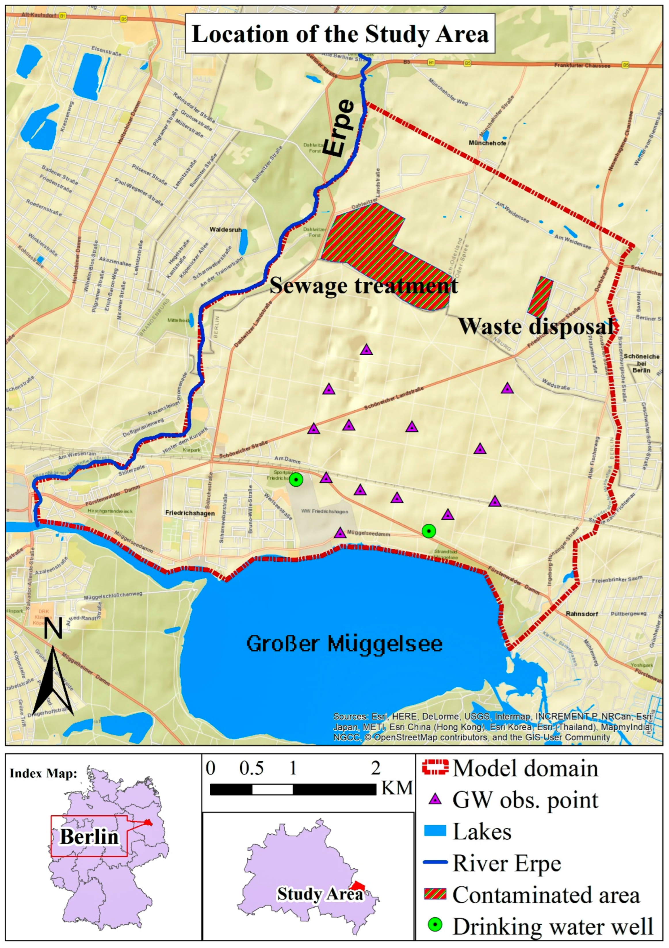
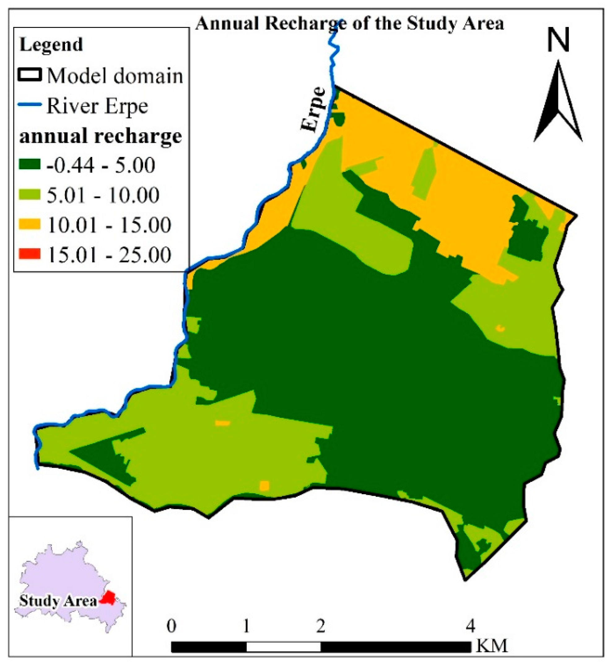
The groundwater problem can be described by the set of differential equations for flow balance in the model domain and at the boundary of the model domain [20,21,22,23,24]:
x 1 k 11 h x 1 + x 2 k 22 h x 2 + w = s s h t
where kii (m/s) is hydraulic conductivity along xi coordinate i = 1, 2; h is hydraulic head; w is volumetric flux (source/sink term); Ss is specific storage of the soil material (porous material); x1 and x2 are the Cartesian coordinates; and t is the time coordinate. For 2D problems with constant hydraulic conductivity in each coordinate direction, the equation can be simplified to:
k 11 2 h x 1 2 + k 22 2 h x 2 2 + w = s s h t
For steady groundwater flow the equation can be simplified to:
k 11 2 h x 1 2 + k 22 2 h x 2 2 + w = 0
Boundary conditions can be h = h0, i.e., Dirichlet boundary condition with given head; q = qB, i.e., Neumann boundary condition with given flux; and q = f(h), i.e., Cauchy boundary condition with flux depending on the head [25,26,27,28,29]. Finite element method is used to discretize the differential equation in FEFLOW [30,31]. A direct frontal solver can be used to resolve the set of linear algebraic equations that result from the typical Galerkin approximation. The Picard iterative technique with options for relaxation is used to solve the nonlinear algebraic equations that result from coupled instances [32,33,34,35,36,37,38,39]. Time is discretized using a straightforward finite difference algorithm.

2.1. Study Area

Near Friedrichshagen, a small German town in the southeast of Berlin, nitrate contamination has been found. Two water supply wells have an increasing concentration [23,24]. There are two possible places where the contamination came from: the first is a group of desolate sewage fields near a wastewater treatment facility in an industrial area northeast of town. Further east is an abandoned trash disposal plant, which is the other potential source. To assess the overall risk to groundwater quality and to calculate the possible pollution, a three-dimensional groundwater flow and pollutant transport model is set up. The town is surrounded by many natural flow boundaries, such as rivers and lakes (Figure 1). There are two small rivers that run north/south on either side of Friedrichshagen that can act as the eastern and western boundaries. Lake Müggelsee can limit the model domain to the south. The northern boundary is chosen along a northwest/southeast hydraulic contour line of groundwater level north of the two potential sources of the contamination. [35,36,37,38,39,40,41,42,43,44,45]. The geology of the study area is comprised of quaternary sediments. The hydrogeologic system contains two main aquifers separated by an aquitard. The top hydro stratigraphic unit is considered to be a sandy unconfined aquifer up to 7 m thick. The second aquifer located below the clayey aquitard has an average thickness of approximately 30 m. The northern part of the model area is primarily used for agriculture, whereas the southern portion is dominated by forest. In both parts, significant urbanized areas exist.

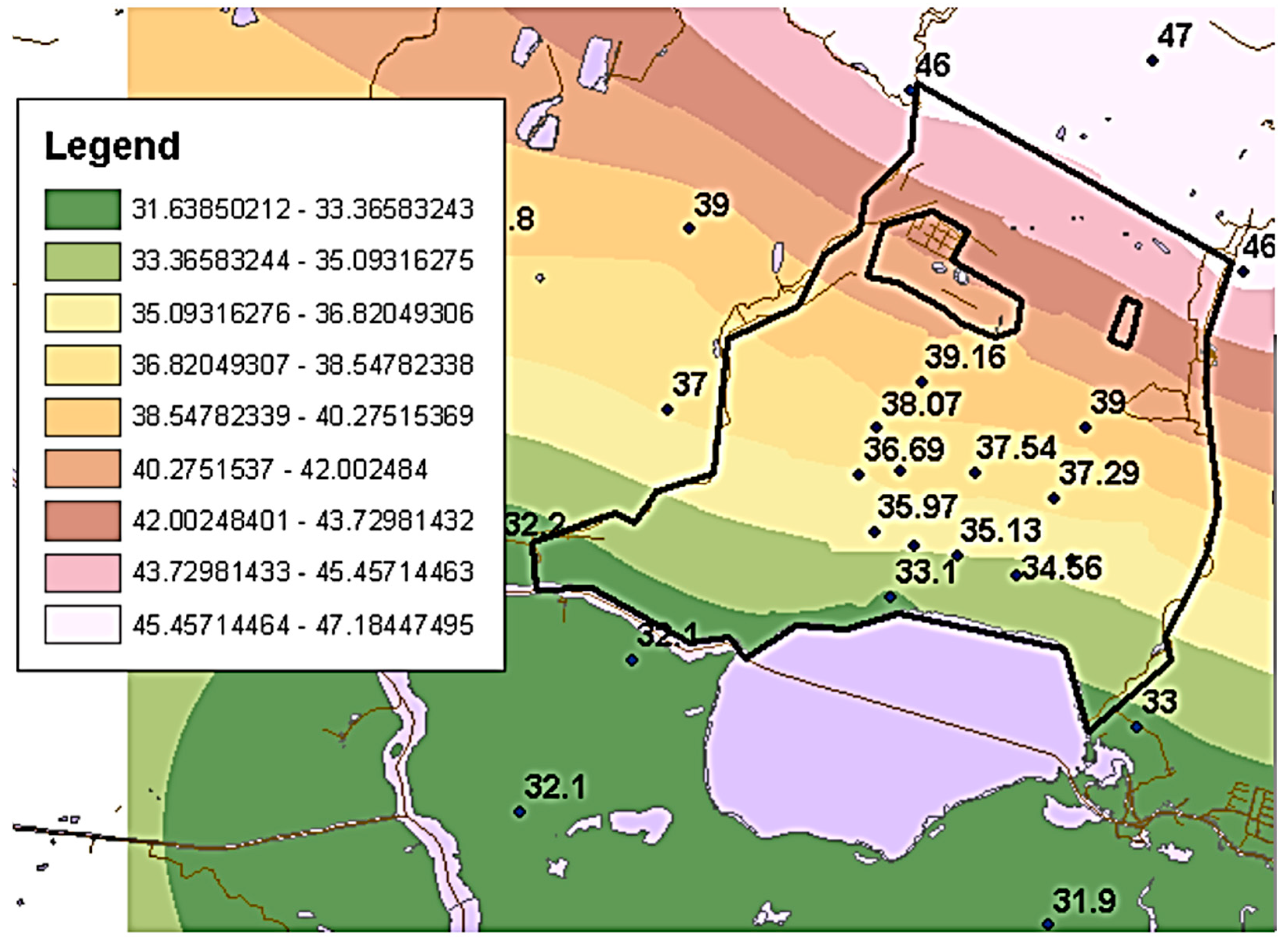
2.2. Data Preprocessing

The following information was used to build the model named as Data underwent processing using ArcGIS. A shapefile named annual recharge describes regions (polygons) with varying groundwater recharge over time. A shapefile named average recharge identifies polygonal regions with dry, average, or wet groundwater recharge. The shapefile (points) “boreholes” describe drilling points with a sediment core, with each point’s x, y, and vertical absolute positions (relative to a reference zero) and the material labeled in accordance with a laboratory sieving test, as well as the material’s transmissive and pervious properties. A drinking water well is defined by a shapefile (points) that includes details such as the radius and pumping rate. Elevations is a shapefile (points) that displays the elevation of common geological properties and was created using surface survey and drilling data. With groundwater measurement stations, the shapefile (points) known as GW measuring describes the recorded groundwater level (average values). A shapefile named as nitrate concentration which is a .tiff file, contains details about the nitrate measurement sites and their associated values while displaying the overall region.
As there are multiple rivers, streams, and lakes in the region, their location can help to identify a suitable modeling domain. In Germany, most waterbodies are fed by groundwater and, thus, their hydraulic head can help to define the boundary condition and modeling domain. The map of the annual recharge of the study area is shown in Figure 2. River water is, like groundwater, subject to gravitational forces and, therefore, generally follows the surface elevation. Where river and groundwater move in parallel, the outer groundwater modeling domain can be delineated along the river, as they can be assumed to move in parallel and thus be represented as an impermeable boundary. The remaining domain boundaries can be found by identifying stable groundwater isolines or waterbodies, such as lakes, that are well connected (same elevation as the groundwater level). At these boundaries, the Dirichlet boundary condition can be set, if no other information is known.
The well-connected Spree River and Lake Müggelsee, which form the southern border, entirely govern the head along that border. These bodies of water have a significant link to the subterranean water. One of the options to determine a value for a first sort (Dirichlet) of hydraulic head boundary condition is the constant lake water level of 32.1 m. The boundaries are formed by two minor rivers, the “Erpe” or the Neuenhagener Mühlenfliessen (Erpe) on the western side and the “Fredersdorfer Mühlenfliessen” on the eastern side. It was hypothesized that these minor creeks flow parallel to the GW because they roughly follow the groundwater flow direction and the surface contour. Under typical low flow circumstances, no water exchange over this boundary is anticipated, hence a no flow border condition can be assumed. Since there are no nearby natural boundary conditions, such as a water divide, a groundwater head contour line was employed; for example, a hydraulic head of 46 m. Only along the same contour line does this border condition hold true.
The groundwater measurement stations that are inside the modeling domain were located for the calibration (Figure 3). Contaminated area was also delineated in ArcGIS inside the model domain. Borehole data from bore hole shape file was used to plan the 3D conceptual design and hydrological structure of different systems of the model, such as aquifer, aquitards, and aquiclude. According to the soil properties, material properties (e.g., conductivity) can be determined.

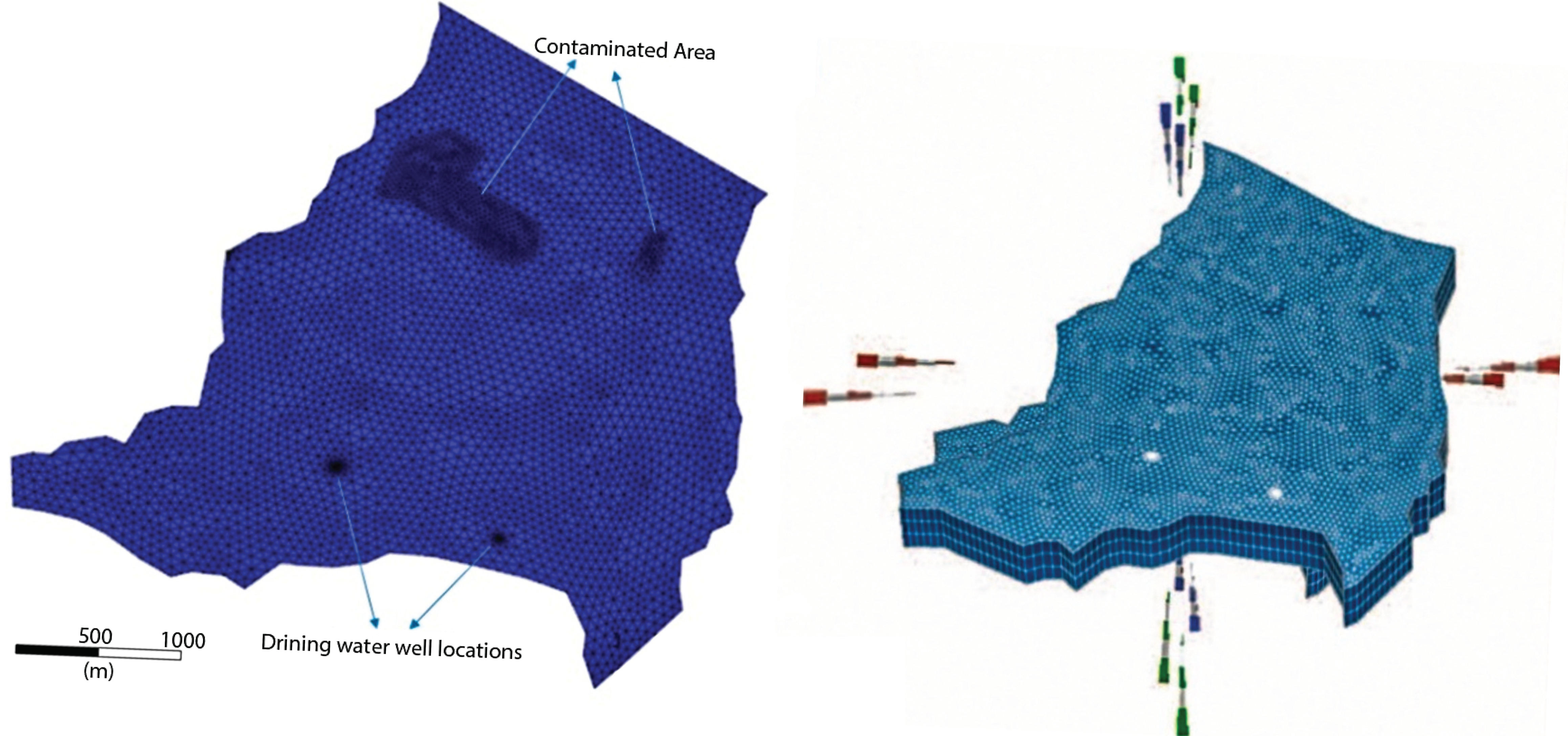
2.3. FEFLOW Model Setup

At the beginning, a steady model was set and simulated to obtain the initial condition for the hydraulic head and pressure distribution for the transient model. The first step of the model set up in FEFLOW is the creation of super mesh. For creating super mesh, necessary maps are imported. All maps were prepared in shapefiles using ArcGIS. Shapefiles contain necessary polygons or poly points which feature the exact boundary of areas within the domain, the domain itself, and wells. Calibration and sensitivity analysis can also be conducted using the steady model.On the other hand, the transient model was used for the calibration and sensitivity analysis due to slight modification in mesh quality. The transient model included mass transport of the mass within the contaminated area, transient data for the drinking water well pumps, and a time series for the annual recharge. In the most straightforward scenario, the super mesh includes a specification of the outer model border. The position of pumping wells, the boundaries of regions with various qualities, or the courses of rivers are other geometrical aspects that may be taken into account while creating the finite-element mesh. The polygons, lines, and points provided by the super mesh can also be utilized later to specify boundary constraints or material qualities. Three different sorts of features—polygons, lines, and points—may be found in a super mesh. The borders of the model region were defined using a polygon. The necessary polygons were directly loaded from the map shapefiles. Before generating the finite-element mesh, the well locations were also included in the super mesh. The domain polygon was separated into multiple aligned polygons with shared vertex and no gap between them to avoid overlapping using “split polygon” function in FEFLOW.
Using split polygon tool, the super mesh was started with the first vertex at the outer edge of the domain near the contaminated areas; then, the edge of the contaminated area was clicked and the upper end of the shape was traced. This continued to the second contaminated area and finished at the opposite edge of the domain. The process was then repeated and the super mesh was started at the last point from the previous split and traced all the way back to the original vertex again. While finishing at the opposing side of the domainit was finalized by clicking enter. The super mesh was used to determine the outside border and other geometrical restrictions before creating the finite-element mesh while using front, triangle, Grid Builder and transport mapping (quadrilateral mode only). Each of the mesh-generation algorithms has its specific property settings. The mesh generation is based on an approximate number of elements to be generated, either for the entire mesh or for each of the polygons. Mesh generation typically is an iterative process, where the generator settings and element numbers are changed until a satisfactory finite-element mesh is obtained. For improving the quality of mesh, obtuse angles in finite elements were avoided. The more obtuse the angle, the poorer the solution quality at the corresponding node. Keeping this in mind, obtuse angles of the triangles were removed by flipping edge technique. The transitions from the course to fine parts of the mesh were kept smooth. Fine mesh was accomplished which covered the physical processes in sufficient detail (e.g., around wells, in zones of contaminant movement, and beside the river). Using Grid Builder as a mesh-generating algorithm, 5000 elements were created in total. Local refinement was performed in well locations and contaminated areas. Delaunay triangulation is an important aspect for the quality of mesh. Delaunay criteria violation was avoided by using flipping edge technique or moving the nodes where necessary.
Up until this point, we only took the model’s top perspective into account and ignored its vertical orientation. This 2D geometry serves as the foundation for the creation of a multi-layered 3D model. A map-based interpolation is used to determine the top and bottom elevations of the layers (point-based data). Three geological strata were taken into consideration for the model in this study. The ground surface on top and an aquitard at the bottom restrict an upper aquifer. Below the aquitard lies a second aquifer that is covered by an unidentified low permeability unit of unknown thickness. This lower stratigraphic stratum is not included in the simulation since it is thought to be impenetrable. Layers are three-dimensional objects that often depict aquifers and aquitards, among other geological formations. Slices are the top- and bottom-model boundaries as well as the interfaces between layers. You may see that the vertical resolution for the transient model was later improved by adding an additional layer to the upper slice, between the second and third slices, at a distance of 10 cm. By regionalizing the elevation data found in map files, this raw geometry was given its actual shape. At first the elevation map (shapefile) was linked to the geometrical property of elevation of FEFLOW in the data panel. To regionalize the point data, Akima was specified as interpolation method with the following properties: linear interpolation, three neighbors, and zero under- or overshooting. The values of elevation were assigned to all nodes. In this same fashion, other necessary shape files were linked with their respective properties (Figure 4).
The Problem Class page defines the FEFLOW model’s primary type. Standard (saturated) groundwater flow equation (Darcy equation) was chosen. Steady state simulation for flow was selected for steady analysis. Unconfined aquifer was chosen under free surface problem class. The first slice of the model was changed to “phreatic”, and others were changed to “dependent”. A residual water depth for unconfined layers of 5 cm was specified. The proper boundary conditions were used to compute the hydraulic head distribution between the upstream and downstream boundary. They were preserved in a very straightforward manner for the sake of simplicity. The head along the southern border is entirely under the administration of Lake Müggelsee. The value for the first sort (Dirichlet) of hydraulic head boundary condition is determined by the lake’s water level of 32.1 m. In place of a natural boundary condition, such as a water split at the northern border (hydraulic head = 46 m), a head contour line was employed. On the other side, the model’s western and eastern bounds are defined by two very small rivers, the Fredersdorfer Mühlenfliessen and the Neuenhagener Mühlenfliessen. We inferred that these severely congested streams served as boundary streamlines, because they generally correspond to the direction of groundwater flow. Since there should be no exchange of water across this barrier, a no-flow boundary condition is presumptive. Finally, two wells with a 1000 m3/d pumping rate and a radius of 0.2 m were placed in the model’s southern region. These correspond to a huge number of genuine well fields. The wells were produced using a map; however, the hydraulic head boundary criteria were manually input. All information needed for the material (elemental) properties were provided in the borehole shapefile. It can be used for linking the parameter to the corresponding material property in the data panel. Otherwise, in case of a homogenous value throughout the entire layer, it is quick to select the entire layer and then assign the value manually. At the beginning the material property, namely, conductivity (cm/s), for complete layer was determined as follows (Table 1):
By interpolating data from field samples in the x direction for all slices, the hydraulic conductivity was determined. The map of borehole drilling points was linked with the conductivity in FEFLOW. For regionalizing the point data, Akima was specified as interpolation method with the properties of linear interpolation, three neighbors, and zero under- or overshooting. Logarithmic interpolation was activated in FEFLOW. In total, 10% of the conductivity in x and y direction for the conductivity in z direction was used for all elements. Before running the file, the observation points provided were added for calibration, by loading them into the maps file and converting them into observation points. Finally, before running the steady model, mesh quality (max. interior angle, Delauney criterion, smoothing mesh, mesh refinement) was tested. For setting up the transient model, some modifications are required in the problem setting section of FEFLOW. Simulation time was adopted as 7300 days for transient model and the fluid flow was considered as transient. The hydraulic head initial conditions had already been calculated from the basic steady model. Initial condition for mass distribution at the contaminated site was provided from the map (shapefile) containing measured nitrate values at the contaminated site. The map was linked to the parameter of mass concentration. For regionalization of the data, inverse distance as data regionalization with four neighbors and an exponent of two were chosen. The nodes in the polygon delineating the contaminated area were selected and the values of contamination were assigned. A zero mg/l Dirichlet BC for the mass transport at the southern and northern boundary were selected. Minimum mass flow constraint was set to 0 g/d. Applying a set concentration is preferred over allowing polluted water to flow freely. Applying a constraint can be used to accomplish the dynamic modification of the mass transport boundary condition based on the flow direction. In this scenario, a constraint is employed to set a minimum or maximum value for the mass flow at a given concentration. The restriction for this investigation is specified to exclusively apply the concentration boundary condition to inflowing water, limiting the mass flux to a minimum value of 0 g/d. The wells in this model have a time-dependent pumping regime, which was loaded as a time series. Proper time series was imported in FEFLOW. As the annual rainfall data show a significant variability during the simulated period, the groundwater recharge is assumed to be time-varying in the model. The file recharge_annual.shp contains the spatial distribution of the approximated recharge for annual periods, each in a separate attribute field. Necessary parameter association was performed considering the time series. Porosity was considered to be 0.2, longitudinal dispersivity to be 70 m, and transverse dispersivity to be 7 m. Finally, the simulation was performed, keeping a record of process variables such as hydraulic conductivity, pressure head, mass concentration, etc.

3. Results and Discussion

A chart of the hydraulic head history was produced for the analysis of the result quality. The values from the chart were imported to MS Excel. Different hydraulic head values at various observation points were loaded. A plot was created for observed hydraulic head vs. simulated hydraulic head values at different observation points. The correlation between simulated and observed head value was found to be y = 1.289x − 2.7373 and the value of the correlation coefficient R2 was found to be 0.8916. R2 is a statistical measure of how close the data are to the fitted regression line. In general, the higher the R2, the better the model line fits the data given. Calibration is not needed, due to R2 being 0.8916, indicating there is a good fit (R2 = 1 indicates perfect correlation), as shown in Figure 5.

3.1. Sensitivity Analysis

A sensitivity analysis has been carried out with the final model (transient) where the Erpe River was incorporated. The material property, namely, the transfer rate-in and transfer rate-out, was used for the analysis. The base case is the final model with the river water level as boundary condition. Results such as hydraulic head, mass concentration, and pressure were recorded, and the impact of the change in the material property on these process variables was analyzed. The material property was changed in different percentages along with the western border and, as a result, the change in percentage of the process variables were observed. An observation point was set up to record the process variables (Figure 6). The process variables were observed for 20 years (end of the simulation period).
By analyzing the response in the process variable (hydraulic head) in Table 2 and Table 3, it can be concluded that the model is not sensible to the changes in the transfer rate, both in and out, and that this property does not influence the simulation results. Due to the absence of a transfer boundary condition, no impact was found. Although, it was found that, with the changing values in the property with different combinations, the result was almost the sameas the previous hydraulic head, mass concentration, and pressure analysis. Models were also set up for extremely higher values and for absolutely zero value of the transfer rate in and transfer rate out to test if the model failed or not (Table 4). However, using the values mentioned in the following table, the model did not fail.
Sensitivity analysis of a different material property, namely, specific storage (compressibility) was also performed. The default value was 0.0001 L/m. Specific storage describes the change in volumetric water content in an aquifer induced per unit change in hydraulic head under saturated conditions. Along with specific yield, specific storage describes the storage properties of an aquifer. As in unconfined layers, specific yield typically exceeds specific storage by far; the influence of this parameter in aquifers with phreatic surfaces is usually negligible. Different percentage changes in specific storage were adopted. An observation point near the contamination area was set up to record the change in process variables (hydraulic head, pressure, and mass transport). A different model was simulated using various specific storage parameters (e.g., specific storage = 0.0001 (base case), 0.1, 1, 50, 100 1/m) (Figure 7). The most sensitive process variable was found to be mass transport.

3.2. Flood Control Strategies

Three types of mitigation measures were considered. These are (1) installation of pumping well where the hydraulic level rises high (almost 1 m below the surface level); (2) barrier; and (3) drainage around the flood prone area (near urbane settlement around the southwestern area of the model). A pumping well with a water withdrawal capacity of 2000 m3/d and a radius of 0.5 m was installed in the mitigation model scenario. A pumping well was found to be a good solution for the local region. A pumping well cannot mitigate or lower the groundwater table over a wide region. For instance, the pumping well can be used for a small region, such as an area of 1 square kilometer. The impact of a pumping well on the hydraulic head is very localized. However, this is a very effective technique to lower the hydraulic head over a small area.
On the other hand, drainage and a barrier also exert an influence on the reduction of the hydraulic head. Compared to a pumping well, their effectiveness was found to be small. This can clearly be seen in the following figures, where comparison of mitigated measures using a pumping well and barrier are illustrated. Up to 1.5 m of reduction of hydraulic head can be achieved using a pumping well, whereas up to 200–300 cm reduction of hydraulic head can be achieved by installing a barrier (Figure 8 and Figure 9). Mitigation measures with drainage were also found to be very ineffective. Considering the bottom of the foundation level to be −1.5 m for all structures, on an average basis, a pumping well was found to be the most effective solution between a barrier or drainage.
Moreover, the cost–benefit point of view also delineates that a pumping well is more cost-effective. The cost of construction of a well at a specific location is much less than constructing a wall of up to 3 m height or a drainage channel up to 2.5 m deep. On the other hand, approximately 935 m of long barrier, or drainage channel, had to be constructed to obtain a reduction in hydraulic head, whereas only a single pumping well was found to be sufficient for reducing the hydraulic head over a small region.
Mass (nitrate) transport was varied due to the incorporation of the river water entrance as a boundary condition at the western part of the model (Figure 10). Mass transport was shown to be faster and more frequently used in 20 years (7300 years) compared to the case where river was not considered. For this reason, more nitrate concentration was observed at the observation point viewing the river, which is shown in the above figure. Although groundwater flooding due to rising river water seldom occurs, it can become crucial when the river is heavily flooded. Groundwater flooding occurs as a result of water rising up from the underlying rocks or from water flowing from the river. This tends to occur after long periods of sustained high rainfall. Higher rainfall means more water will infiltrate into the ground and cause the water table to rise above normal levels. When a house is knee deep in water, groundwater flooding looks the same as river flooding. However, the flooding processes are different, and management of the problem needs to reflect this. Groundwater flooding often persists long after river flooding has subsided. Even “underground flooding” can affect infrastructure and services such as underground trains and sewers. When water reaches the surface, the destructive potential also rises. Flooded sewers can overflow, causing contaminated water to emerge into streets, gardens, and homes. Property can be damaged, and people’s lives can be turned upside down. Groundwater flooding is most likely to occur in low-lying areas underlain by permeable rocks (aquifers).
In this study domain, no groundwater overtopping of the surface was observed by the simulation of a groundwater model using FEFLOW. Maximum hydraulic head was found over the urban settlement area situated at the southwestern part of the study domain. By subtracting the hydraulic head from the surface elevation groundwater, the depth was found, and the minimum value was found to be approximately 1 m below the surface level. This level can be crucial at the urban settlement area where many single-storied buildings are situated. A pumping well was found to be more effective compared to a barrier construction and drainage installment technique, both technically and from a cost–benefit point of view. A pumping well was found to be suitable for reducing hydraulic head locally, thus lowering the groundwater level. Data preprocessing is a very important step for groundwater modelling in FEFLOW. Sufficient data are needed over the whole domain. Otherwise, due to a greater interpolation, predicting the process variables over a long period may produce inaccurate results. Material properties should be considered according to the soil profile data. There might be different soil types existing in a single domain. Uniform material groundwater flooding looks the same as river flooding.

4. Conclusions

The simulation of the groundwater model utilizing FEFLOW in this study did not show any groundwater overtopping of the surface. The urban settlement area, which is located in the southwestern corner of the study domain, had the highest hydraulic head. The minimal value for groundwater depth was determined to be about 1 m below the surface level by subtracting the hydraulic head from the surface height. This level can be quite important in metropolitan areas where there are many single-story structures. From a technical and cost–benefit perspective, a pumping well was shown to be superior to the building of a barrier or comparing to a drainage installation techniques. It was discovered that a pumping well might effectively lower the local hydraulic head and groundwater level by reducing hydraulic head.
Data preprocessing is a very important step for groundwater modelling in FEFLOW. Sufficient data is needed over the whole domain. Otherwise, due to a greater interpolation, predicting the process variables over a long period may produce inaccurate results. Material properties should be considered according to the soil profile data. There might be different soil types existing in a single domain. However, uniform material property was considered in our model scenario. Considering the borehole data, the number and thickness of aquifers was considered in the model. Due to the differences in boundary conditions, the model’s result may vary significantly. The total time period for the model was 20 years. In this period of time, process variables such as hydraulic head and pressure head reach at a steady state (similar to the initial condition). During high precipitation, changes in the process variables were high. Spatial distribution of hydraulic head and spread of contamination were studied in a period of 20 years. Due to the consideration of rising river water, GW flooding was observed. The urban settlement located at the southwestern side of the study area is flood prone. Considering the land use and the cost of different mitigation possibilities, local mitigation by a water pumping well at the urban settlement area was found to be most efficient. Groundwater flooding occurs as a result of water rising up from the underlying rocks or from water flowing from the river. Although groundwater flooding due to rising river water seldom occurs, it can become crucial when the river is heavily flooded. Even “underground flooding” can affect infrastructure and services such as underground trains and sewers. No groundwater overtopping of the surface was observed by the simulation of a groundwater model using FEFLOW. Maximum hydraulic head was found over the urban settlement area situated at the southwestern part of the study domain. As a result, a pumping well was found to be more effective in both technically and from a cost–benefit point of view, compared to a barrier construction and drainage installment technique.

Author Contributions

Conceptualization, R.K.; methodology, R.K. and M.M.S.Y.; investigation, R.K. and M.M.S.Y.; formal analysis, R.K.; resources, R.K.; data preparation, R.K.; writing—original draft preparation, M.M.S.Y. and R.K; writing—review and editing, M.M.S.Y., and R.K.; visualization, R.K. and M.M.S.Y. All authors have read and agreed to the published version of the manuscript.

Funding

This research received no external funding.

Institutional Review Board Statement

Not applicable.

Informed Consent Statement

Not applicable.

Data Availability Statement

Data collected for the study can be made available upon request from the corresponding author.

Acknowledgments

This paper and the research behind it would not have been possible without the exceptional support of Md Abdullah Al Mehedi, a candidate in the Department of Civil and Environmental Engineering at Villanova University. His enthusiasm, knowledge and exacting attention to detail have been an inspiration and kept the work on track from my first encounter to the final draft of this paper. He contributed to the model formulation, strategic planning on model simulation, structuring and interpreting the results and identifying future direction and limitations. We are grateful to his valuable ideation and contribution.

Conflicts of Interest

The authors declare no conflict of interest.

References

  1. Macdonald, D.; Dixon, A.; Newell, A.; Hallaways, A. Groundwater Flooding within an Urbanised Flood Plain. J. Flood Risk Manag. 2011, 5, 68–80. [Google Scholar] [CrossRef] [Green Version]
  2. Lu, C.; Ji, K.; Wang, W.; Zhang, Y.; Ealotswe, T.K.; Qin, W.; Lu, J.; Liu, B.; Shu, L. Estimation of the Interaction between Groundwater and Surface Water Based on Flow Routing Using an Improved Nonlinear Muskingum-Cunge Method. Water Resour. Manag. 2021, 35, 2649–2666. [Google Scholar] [CrossRef]
  3. Kumar, C. Climate Change and Its Impact on Groundwater Resources. Res. Inventy Int. J. Eng. Sci. 2012, 1, 43–60. [Google Scholar]
  4. Yazdan, M.M.S.; Kumar, R.; Leung, S.W. The Environmental and Health Impacts of Steroids and Hormones in Wastewater Effluent, as Well as Existing Removal Technologies: A Review. Ecologies 2022, 3, 206–224. [Google Scholar] [CrossRef]
  5. Nemčić-Jurec, J.; Ruk, D.; Oreščanin, V.; Kovač, I.; Ujević Bošnjak, M.; Kinsela, A.S. Groundwater Contamination in Public Water Supply Wells: Risk Assessment, Evaluation of Trends and Impact of Rainfall on Groundwater Quality. Appl. Water Sci. 2022, 12, 172. [Google Scholar] [CrossRef]
  6. Abd-Elaty, I.; Negm, A.; Hamdan, A.M.; Nour-Eldeen, A.S.; Zeleňáková, M.; Hossen, H. Assessing the Hazards of Groundwater Logging in Tourism Aswan City, Egypt. Water 2022, 14, 1233. [Google Scholar] [CrossRef]
  7. Mehedi, M.A.A.; Yazdan, M.M.S. Automated Particle Tracing & Sensitivity Analysis for Residence Time in a Saturated Subsurface Media. Liquids 2022, 2, 72–84. [Google Scholar] [CrossRef]
  8. Zurqani, H.A.; Al-Bukhari, A.; Aldaikh, A.O.; Elfadli, K.I.; Bataw, A.A. Geospatial Mapping and Analysis of the 2019 Flood Disaster Extent and Impact in the City of Ghat in Southwestern Libya Using Google Earth Engine and Deep Learning Technique. Environ. Appl. Remote Sens. GIS Libya 2022, 205–226. [Google Scholar] [CrossRef]
  9. Mehedi, M.A.A.; Reichert, N.; Molkenthin, F. Sensitivity Analysis of Hyporheic Exchange to Small Scale Changes in Gravel-Sand Flumebed Using a Coupled Groundwater-Surface Water Model. Available online: https://meetingorganizer.copernicus.org/EGU2020/EGU2020-20319.html (accessed on 30 July 2022).
  10. Moran, B.J.; Boutt, D.F.; McKnight, S.V.; Jenckes, J.; Munk, L.A.; Corkran, D.; Kirshen, A. Relic Groundwater and Prolonged Drought Confound Interpretations of Water Sustainability and Lithium Extraction in Arid Lands. Earth’s Future 2022, 10, e2021EF002555. [Google Scholar] [CrossRef]
  11. Ma, X.; Dahlke, H.; Duncan, R.; Doll, D.; Martinez, P.; Lampinen, B.; Volder, A. Winter Flooding Recharges Groundwater in Almond Orchards with Limited Effects on Root Dynamics and Yield. Calif. Agric. 2022, 76, 70–76. [Google Scholar] [CrossRef]
  12. Mehedi, M.A.A.; Yazdan, M.M.S.; Ahad, M.T.; Akatu, W.; Kumar, R.; Rahman, A. Quantifying Small-Scale Hyporheic Streamlines and Resident Time under Gravel-Sand Streambed Using a Coupled HEC-RAS and MIN3P Model. Eng 2022, 3, 276–300. [Google Scholar] [CrossRef]
  13. Basu, B.; Morrissey, P.; Gill, L.W. Application of Nonlinear Time Series and Machine Learning Algorithms for Forecasting Groundwater Flooding in a Lowland Karst Area. Water Resour. Res. 2022, 58, e2021WR029576. [Google Scholar] [CrossRef]
  14. Kumar, C. An Overview of Commonly Used Groundwater Modelling Software. Int. J. Adv. Sci. Eng. Technol. 2019, 6, 7854–7865. [Google Scholar]
  15. Ahmad, M.; Al Mehedi, M.A.; Yazdan, M.M.S.; Kumar, R. Development of Machine Learning Flood Model Using Artificial Neural Network (ANN) at Var River. Liquids 2022, 2, 147–160. [Google Scholar] [CrossRef]
  16. Yazdan, M.M.S.; Ahad, M.T.; Kumar, R.; Mehedi, M.A.A. Estimating Flooding at River Spree Floodplain Using HEC-RAS Simulation. Preprints 2022, 5, 410–426. [Google Scholar] [CrossRef]
  17. Mehedi, M.A.A.; Khosravi, M.; Yazdan, M.M.S.; Shabanian, H. Exploring Temporal Dynamics of River Discharge using Univariate Long Short-Term Memory (LSTM) Recurrent Neural Network at East Branch of Delaware River. Preprints 2022, 9, 202. [Google Scholar] [CrossRef]
  18. Yazdan, M.M.S.; Khosravia, M.; Saki, S.; Mehedi, M.A.A. Forecasting Energy Consumption Time Series Using Recurrent Neural Network in Tensorflow. Preprints 2022, 2022090404. [Google Scholar] [CrossRef]
  19. Macdonald, D.M.J.; Bloomfield, J.P.; Hughes, A.G.; MacDonald, A.M.; Adams, B.; McKenzie, A.A. Improving the understanding of the risk from groundwater flooding in the UK. In Proceedings of the European Conference on Flood Risk Management, Oxford, UK, 30 September–2 October 2008. [Google Scholar]
  20. Cobby, D.; Morris, S.; Parkes, A.; Robinson, V. Groundwater flood risk management: Advances towards meeting the requirements of the EU floods directive. J. Flood Risk Manag. 2009, 2, 111–119. [Google Scholar] [CrossRef]
  21. Pinault, J.-L.; Amraoui, N.; Golaz, C. Groundwater-induced flooding in macropore-dominated hydrological system in the context of climate changes. Water Resour. Res. 2005, 41, 1029–1036. [Google Scholar] [CrossRef] [Green Version]
  22. Finch, J.W.; Bradford, R.B.; Hudson, J.A. The spatial distribution of groundwater flooding in a chalk catchment in southern England. Hydrol. Process. 2004, 18, 959–971. [Google Scholar] [CrossRef]
  23. Allocca, V.; Coda, S.; Calcaterra, D.; De Vita, P. Groundwater rebound and flooding in the Naples’ periurban area (Italy). J. Flood Risk Manag. 2022, 15, e12775. [Google Scholar] [CrossRef]
  24. Su, X.; Belvedere, P.; Tosco, T.; Prigiobbe, V. Studying the effect of sea level rise on nuisance flooding due to groundwater in a coastal urban area with aging infrastructure. Urban Clim. 2022, 43, 101164. [Google Scholar] [CrossRef]
  25. Gold, A.C.; Brown, C.M.; Thompson, S.P.; Piehler, M.F. Inundation of stormwater infrastructure is common and increases risk of flooding in coastal urban areas along the US Atlantic coast. Earth’s Future 2022, 10, e2021EF002139. [Google Scholar] [CrossRef]
  26. Naji, L.; Tawfiq, M.; Jabber, A. Solve the Groundwater Model Equation Using Fourier Transforms Method Research Article. Int. J. Adv. Appl. Math. Mech. 2017, 5, 2347–2529. [Google Scholar]
  27. Pinder, G.F. An Overview of Groundwater Modelling. Groundw. Flow Qual. Model. 1988, 224, 119–134. [Google Scholar] [CrossRef]
  28. Yazdan, M.M.S.; Ahad, M.T.; Mallick, Z.; Mallick, S.P.; Jahan, I.; Mazumder, M. An Overview of the Glucocorticoids’ Pathways in the Environment and Their Removal Using Conventional Wastewater Treatment Systems. Pollutants 2021, 1, 141–155. [Google Scholar] [CrossRef]
  29. Tepe, N.; Romero, M.; Bau, M. High-Technology Metals as Emerging Contaminants: Strong Increase of Anthropogenic Gadolinium Levels in Tap Water of Berlin, Germany, from 2009 to 2012. Appl. Geochem. 2014, 45, 191–197. [Google Scholar] [CrossRef]
  30. Kuhlemann, L.; Tetzlaff, D.; Soulsby, C. Urban Water Systems under Climate Stress: An Isotopic Perspective from Berlin, Germany. Hydrol. Process. 2020, 34, 3758–3776. [Google Scholar] [CrossRef]
  31. Wise, D.L. Bioremediation of Contaminated Soils; CRC Press: Boca Raton, FL, USA, 2000; ISBN 9780429078040. [Google Scholar]
  32. García Revilla, M.R.; Martínez Moure, O. Wine as a Tourist Resource: New Manifestations and Consequences of a Quality Product from the Perspective of Sustainability. Case Analysis of the Province of Málaga. Sustainability 2021, 13, 13003. [Google Scholar] [CrossRef]
  33. Richter, D.; Massmann, G.; Taute, T.; Duennbier, U. Investigation of the Fate of Sulfonamides Downgradient of a Decommissioned Sewage Farm near Berlin, Germany. J. Contam. Hydrol. 2009, 106, 183–194. [Google Scholar] [CrossRef]
  34. Kinzelbach, W. Groundwater Modelling: An Introduction with Sample Programs in BASIC; Elsevier: Amsterdam, The Netherlands, 1986. [Google Scholar]
  35. Kumar, C.P. “IJMSET Promotes Research Nature, Research Nature Enriches the World’s Future” Modelling of Groundwater Flow and Data Requirements. Int. J. Mod. Sci. Eng. Technol. 2015, 2, 18–27. [Google Scholar]
  36. Ohara, N.; Steven Holbrook, W.; Yamatani, K.; Flinchum, B.A.; St. Clair, J.T. Spatial Delineation of Riparian Groundwater within Alluvium Deposit of Mountainous Region Using Laplace Equation. Hydrol. Process. 2017, 32, 30–38. [Google Scholar] [CrossRef]
  37. Ling, L.; Jian, C.; Haobo, N.; Li, L.; Leyi, Y.; Yaqiang, W. Numerical simulation of three-dimensional soil-groundwater coupled chromium contamination based on FEFLOW. Hydrogeology & Engineering Geology. Hydrogeol. Eng. Geol. 2022, 49, 164–174. [Google Scholar] [CrossRef]
  38. Ashraf, A.; Ahmad, Z. Regional Groundwater Flow Modelling of Upper Chaj Doab of Indus Basin, Pakistan Using Finite Element Model (FEFLOW) and Geoinformatics. Geophys. J. Int. 2008, 173, 17–24. [Google Scholar] [CrossRef]
  39. Yazdan, M.M.S.; Ahad, M.T.; Jahan, I.; Mazumder, M. Review on the Evaluation of the Impacts of Wastewater Disposal in Hydraulic Fracturing Industry in the United States. Technologies 2020, 8, 67. [Google Scholar] [CrossRef]
  40. Zhao, C.; Wang, Y.; Chen, X.; Li, B. Simulation of the Effects of Groundwater Level on Vegetation Change by Combining FEFLOW Software. Ecol. Model. 2005, 187, 341–351. [Google Scholar] [CrossRef]
  41. Diersch, H.-J.G. FEFLOW: Finite Element Modeling of Flow, Mass and Heat Transport in Porous and Fractured Media; Springer Science & Business Media: Berlin, Germany, 2013. [Google Scholar]
  42. Rahaman, A.Z.; Yazdan, M.M.S.; Noor, F.; Duti, B.M. Establishment of Co-Relation Between Remote Sensing Based Trmm Data and Ground Based Precipitation Data in North-East Region of Bangladesh. In Proceedings of the 2nd International Conference on Civil Engineering for Sustainable Development (ICCESD-2014), KUET, Khulna, Bangladesh, 14–16 February 2014. Deep Convection for Thunderstorm: CAPE and Shear Analysis in Present and Future Climate View Project Seven River Dredging Project: Case of Old Brahmaputra River View Project. [Google Scholar]
  43. Kaur, B.; Binns, A.; Sandink, D.; Gharabaghi, B.; McBean, E. Reducing the Risk of Basement Flooding through Building- and Lot-Scale Flood Mitigation Approaches: Performance of Foundation Drainage Systems. Lect. Notes Civ. Eng. 2022, 250, 471–477. [Google Scholar] [CrossRef]
  44. Hossain, B.M.T.A.; Ahmed, T.; Aktar, N.; Khan, F.; Islam, A.; Yazdan, M.M.S.; Noor, F.; Rahaman, A. Climate Change Impacts on Water Availability in the Meghna Basin. In Proceedings of the 5th International Conference on Water and Flood Management (ICWFM-2015), Dhaka, Bangladesh, 6–8 March 2015. [Google Scholar]
  45. Humnicki, W.; Krogulec, E.; Małecki, J.; Szostakiewicz-Hołownia, M.; Wojdalska, A.; Zaszewski, D. Groundwater impact assessment of Lake Czorsztyn after 25 years of its operation. Arch. Environ. Prot. 2022, 48, 65–78. [Google Scholar] [CrossRef]
Figure 1. Study domain of this study.
J 06 00001 g001
Figure 2. Map of the annual recharge of the study area.
J 06 00001 g002
Figure 3. Observed groundwater level value along with locations and interpolated contour lines in the model domain.
J 06 00001 g003
Figure 4. Model domain showing super mesh with high mesh resolution at the contaminated and drinking water well locations, 3D configuration.
J 06 00001 g004
Figure 5. Correlation between simulated and observed head value.
J 06 00001 g005
Figure 6. Observation location to observe the change in hydraulic head.
J 06 00001 g006
Figure 7. Impact of change in specific storage.
J 06 00001 g007
Figure 8. Comparison of mitigated (well) and flooding scenario. Time period was considered to be 180–200 days.
J 06 00001 g008
Figure 9. Comparison of mitigated (barrier) and flooding scenario. Time period was considered to be 180–200 days.
J 06 00001 g009
Figure 10. Spread of contaminant with and without considering the Erpe River.
J 06 00001 g010
Table 1. Layer components.
ComponentsLayer 1Layer 2Layer 3
In/outflow on top/bottom19.5 cm/sN/AN/A
K_xxN/A2 × 10−2 cm/s1 × 10−4 cm/s
K_yyN/A2 × 10−2 cm/s1 × 10−4 cm/s
K_zzN/A2 × 10−3 cm/s1 × 10−5 cm/s
Drain/fillable porosity0.10.150.1
Table 2. Variation of hydraulic head with changed material property (transfer rate in).
Head from Base Case (m) Changed Head (m) Change in Hydraulic Head (%)Global Change in Material Property (%) (TRI)
35.5535.55−0.001 −100
35.5535.55 −0.001 −50
35.5535.55−0.0003 50
35.5535.55 −0.0006 100
35.5535.55−0.0008 150
Table 3. Variation of hydraulic head with changed material property (transfer rate out).
Head from Base Case (m)Changed Head (m)Change in Hydraulic Head (%)Global Change in Material Property (%) (TRO)
35.5535.550.001−100
35.5535.590.109−50
35.5535.550.000050
35.5535.550.0014100
35.5535.550.0006150
Table 4. Model scenario with high change in material property (transfer rate in and out).
Scenario Name (ID) Transfer Rate in (L/d)Percent Change (%)Transfer Rate Out (L/d)Comments
SnScBase200n/a800Base scenario
SnSc1_TRI_Ex112005004800Change in transfer rate out
SnSc1_TRI_Ex2220010008800
SnSc1_TRI_Ex34200200016,800
Disclaimer/Publisher’s Note: The statements, opinions and data contained in all publications are solely those of the individual author(s) and contributor(s) and not of MDPI and/or the editor(s). MDPI and/or the editor(s) disclaim responsibility for any injury to people or property resulting from any ideas, methods, instructions or products referred to in the content.

