1. Introduction
With the increase of Renewable Energy Sources (RES) the demand for oil and gas has been decreasing. Moreover, 238 GW of installed wind and solar power capacity has been added during 2021, thus demonstrating the ability of RES to overcome the world’s energy crisis [
1,
2]. Likewise, RES provided approximately 29% of the world’s electricity generation [
3].
Wind energy is among the main RES. This energy source already provides a significant portion of the electrical energy consumption in several countries of the European Union. In Latin America and the Caribbean, 4.7 GW were added for a regional total of 33.9 GW. In Mexico, during 2020, only 0.6 GW were added to its installed capacity. Therefore, Mexico, which was considered one of the top 10 installers in Latin America, disappeared from the list [
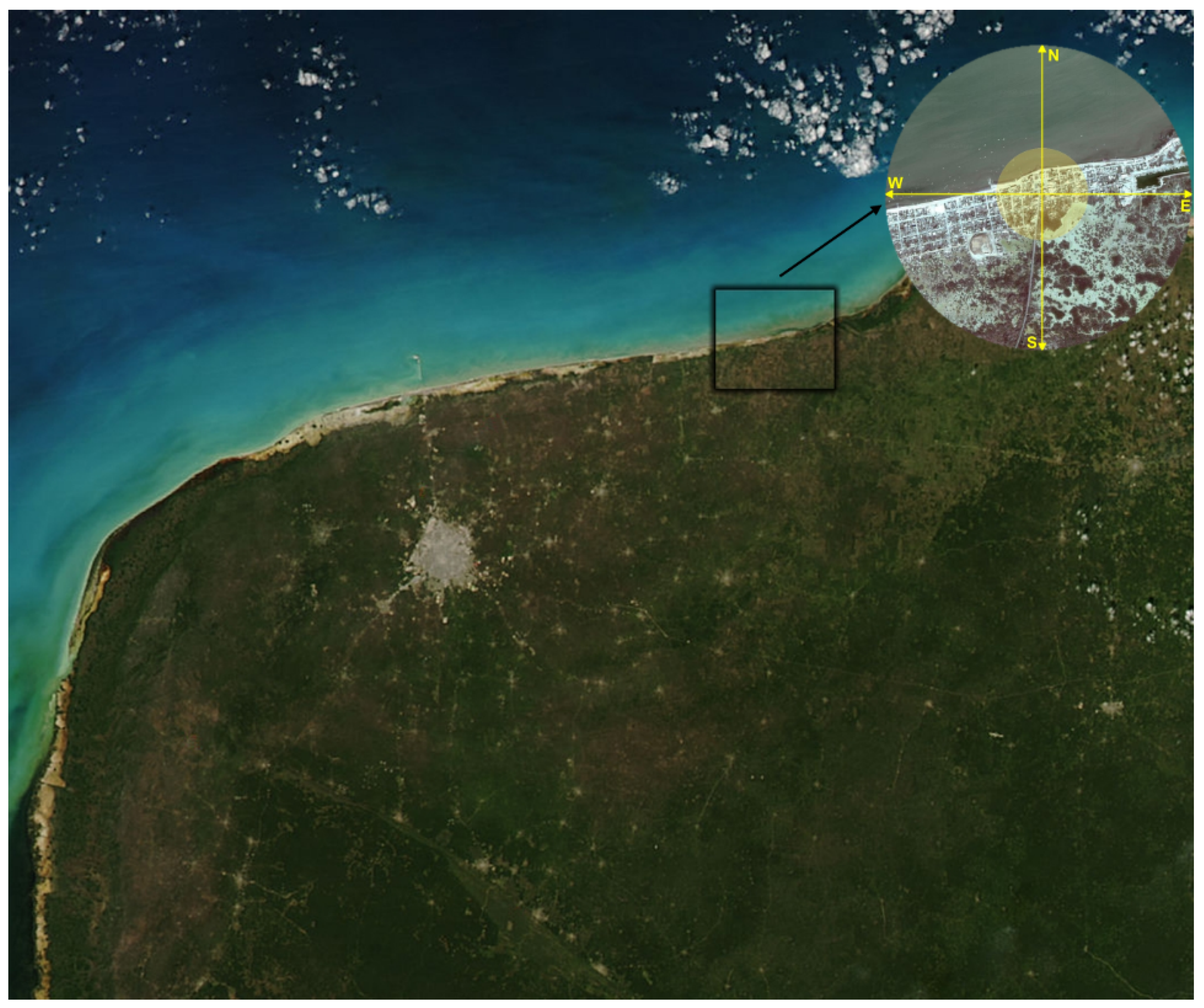
3]. However, many regions in Mexico such as Baja California, Veracruz, Oaxaca, and Yucatan have wind power capacity potential [
4]. Particularly, the Yucatan Peninsula has a technical capacity and annual generation potential of 6125 MW and 14,802 GWh, respectively [
5]. With three wind farms in operation, the state of Yucatan has an installed capacity of 244.7 MW [
6,
7,
8].
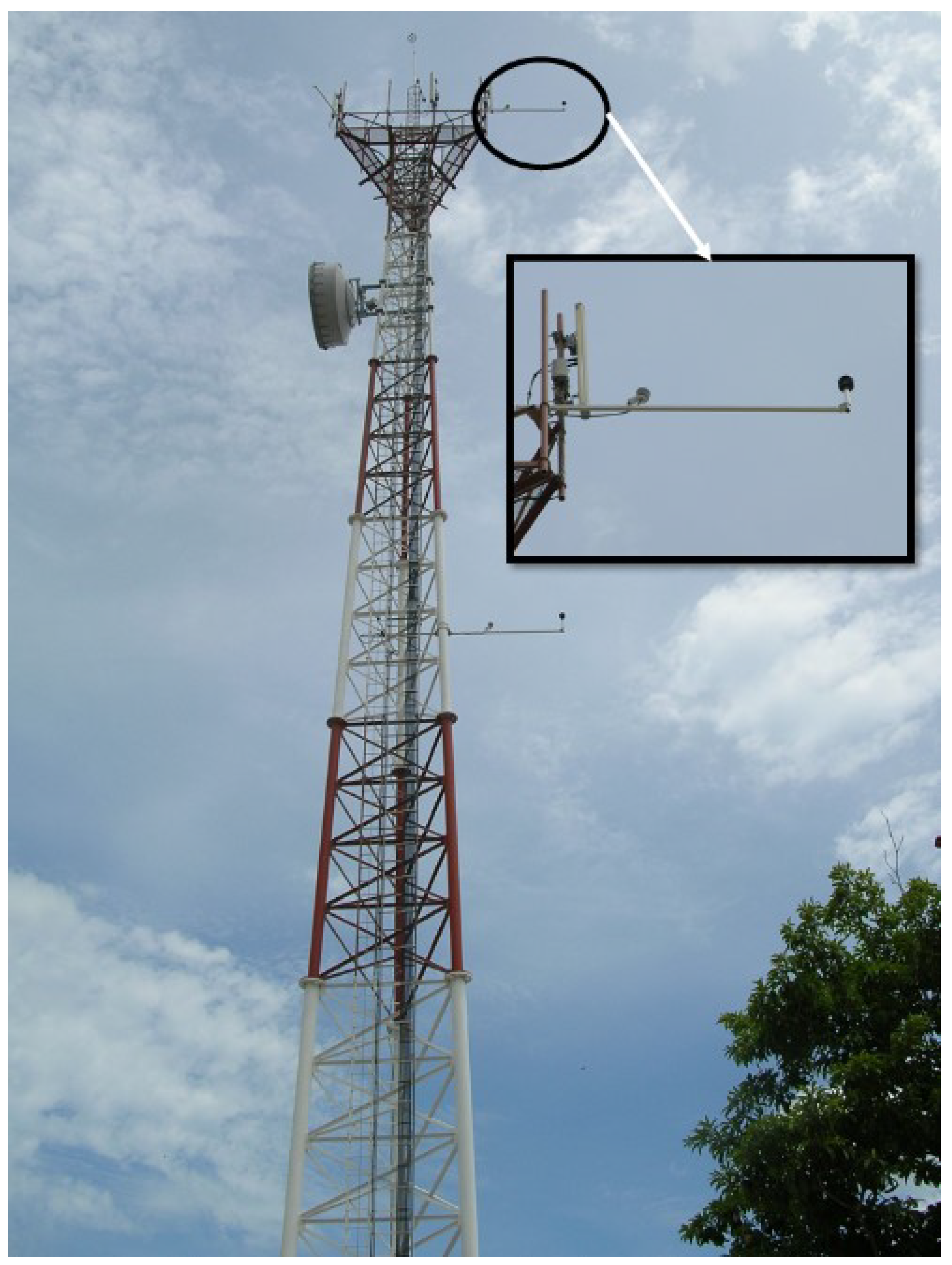
With the installation of wind farms being more frequent in these types of regions (i.e., flat areas and at sea level), a proper evaluation of the wind resource for each determined site is essential for the successful development of the power grid, since the turbine production depends mainly on wind speed. It is possible to calculate energy production by having the turbine power curve and the resource assessment. To carry out this evaluation, the main anemometric variables to be measured are wind speed, wind direction, temperature, and atmospheric pressure (the first two parameters are key values since, as the wind is an airflow, not all the wind is used to generate) [
9]. However, recording wind speed data using different devices as anemometers can present errors due to different wind conditions, which represents a problem in obtaining the best performance from a power grid [
10]. This affects the electricity service and the economy of the people who live in areas such as Yucatan, especially people with low income. To solve this problem, many researchers have developed different mathematical models depending on the lapse of time to be able to anticipate wind conditions. Prediction models, depending on the period, can be classified into very short term (a few seconds to 30 min), short term (30 min to 6 h), medium-term (6 h to 24 h), long term (24 h to 72 h), and very long term (>72 h) [
11,
12,
13,
14,
15,
16].
Another classification is made according to methodology. In this way, the models can be deterministic (or physical), statistical, and hybrid. Physical methods use previous wind power data and Numerical Weather Prediction (NWP) data. These models require a more detailed physical description of the site including roughness, obstacles, temperature, pressure, etc., which makes them computationally complex. This approach requires considerable resources, both computationally and economically since, although the data required are common to all wind forecast models, they will vary with the location of the wind farm and it will be necessary to obtain them for each location. Physical approaches are satisfactory for short-term and long-term forecasting [
16,
17,
18]. Statistical methods are based on historical data series to make a forecast for the next few hours. These models present good results for short periods. Its main disadvantage is that, as the time in the forecast increases, the prediction error also increases. Specifically, these methods can be divided into traditional models, time series based, and Artificial Neural Networks (ANN). The most frequently used statistical models include autoregressive model, moving average, autoregressive moving average (ARMA), autoregressive integrated moving average (ARIMA), exponential smoothing, Markov chain, Generalized Autoregressive Conditional Heteroskedasticity (GARCH), among others [
19,
20,
21,
22]. Hybrid or mixed methods are due to the combination of different approaches (physical and statistical) and different time windows. The main objective of this method is to benefit from each method and improve the accuracy of the forecasts. Although it is not always achieved, it has been proved that there are lower risks in most situations. Among these methods are ANN-ARIMA, wavelet-ANN, wavelet-ARIMA, Kalman filter-ANN (KF + ANN), Wavelet-Support vector machine optimized by genetic algorithm (WT-SVM-GA), Isolation Forest (IF)-deep learning-ANN, CEE-CC-FS, among others [
20,
21,
22,
23,
24,
25].
In particular, the exponential smoothing method has great variability, adaptation, and a large number of applications. This method is characterized by giving weight to the error caused by the forecast and the experimental data and using the previous forecasts to generate the following predictions. Therefore, the latest observations significantly influence the current forecast, as is the case with short-term measurements of wind speed. However, according to works reported in the literature, the use of the exponential smoothing method in the prediction of wind speed is scarce [
19]. In [
19], the authors have analyzed the wind speed data collected in Chetumal, Quintana Roo by using a statistical analysis of the time series and the Single Exponential Smoothing (SES) method. Finally, in the work [
19], the SES method has been compared with the artificial neural network method to prove that the SES method is very useful for wind speed forecasting (in particular for Chetumal, Quintana Roo). In [
26], the authors have developed a combined forecasting system and validated it by comparing it with wind speed data sets from three different wind farms in Penglai, China. Furthermore, in the work [
26], the performance of the model has been proved by contrasting it with an extension of the exponential smoothing method and two machine learning models. In the paper [
27], two-hybrid forecasting systems based on the structural characteristics of wind speed have been proposed to capture the linear and nonlinear factors hidden in wind speed data. This is because the authors have used a decomposition algorithm to eliminate noise from raw data and reconstruct more reliable wind speed time data. So, a linear model based on the exponential smoothing method or autoregressive moving average model captures the linear patterns hidden and a nonlinear model based on the backpropagation neural network extracts the nonlinear patterns hidden in the data.
Although the use of the exponential smoothing method for the development of new forecasting methods for wind speed is scarce, different forecasting methods have been developed based on other traditional methods. In [
10], the authors have evaluated the effects of a set of various moving average filter durations and turbulence intensities on the recorded maximum gust wind speed to present a function dependent on the average duration and turbulence intensity. In [
28], a new forecasting method is proposed by the combination of the local convolutional neural network. The authors have transformed the non-convex problems into convex problems to obtain the globally optimal solutions for the convex problems by using heuristic optimization algorithms. Therefore, a more stable model can be constructed to deal with various wind speed data sets. In the work [
29], the authors have developed a forecasting method to assess and predict wind speed by integrating Sentinel satellite imagery analysis. This process has been carried out by using multi-sensor satellites and machine learning methods. Furthermore, the developed method has been applied to assess wind energy potential around the Favignana island in Sicily, Italy. In [
30], the authors have improved the accuracy of forecasting the short-term wind speed by developing a hybrid wind speed forecasting model based on four modules: crow search algorithm, wavelet transform, feature selection based on entropy and mutual information, and deep learning time series prediction based on long short term memory neural networks. Moreover, the proposed method developed in this work was applied to wind data from Galicia, Spain, and Iran. In [
31], a combined prediction system has been proposed to develop a new forecasting method based on optimal sub-model selection, point prediction based on a modified multi-objective optimization algorithm, interval forecasting based on distribution fitting, and forecasting system evaluation.
From the current state of the art, this work focuses on developing four variants of the exponential smoothing forecasting method to optimize the forecast of wind speed. Thus, it is possible to propose strategies to improve the energy harvested from wind farms (in this case, for Yucatan peninsula wind farms) avoiding the main grid as much as possible. This would support the local economy and improve energy services. Furthermore, these methods can be applied to any kind of data.
This paper is divided into six sections. After the introduction, in
Section 2 the characteristics of the experiment are described (i.e., experimental test set-up and characteristics of the area where the data were collected). In
Section 3, a brief description of the SES method and the Double Exponential Smoothing (DES) method is provided. Later in
Section 4, the optimization of the SES and DES methods is developed and explained. Subsequently, results and discussion of these forecasting methods developed are presented in
Section 5. Finally, the conclusion of this work is given in
Section 6.
4. Proposed Optimization of SES and DES Methods for Wind Speed Data
The non-linear least squares function (Equation (
10)) has been implemented to optimally calculate the parameters
,
, and
for each day of the year according to the experimental data obtained, as an optimization for the SES and DES methods. The minimum daily error of the SES and DES methods was calculated by adjusting the parameters
,
, and
. With these parameters, it is possible to develop variants of the traditional SES and DES methods as described in this section.
where
n is the number of data,
p is the set of parameters of the equations (i.e.,
for (
8) and
for (
9)).
With optimal parameters, two variants from the SES method and two variants from the DES method have been proposed. The first variant for the SES method is given by:
where
where
is the optimal parameter of the day
k and
N is the number of days of the month (i.e.,
N is equal to 28, 30, or 31 depending on the month).
has been calculated by using the command
lsqcurvefit in the software MATLAB
. As can be seen, this variant consists in obtaining the average of the optimal
s corresponding to a month. Then this average is implemented in the classical SES method.
The second variant for the SES method is given by:
In this variant, the classical SES method has been adapted by iterations of the optimal value of , in other words, it is the optimal parameter of the previous day k, the optimum value has been used for the first day of each month ().
Similarly, the variants of the DES method are similar to the variants of the SES method. The first variant of the DES method is given by:
where
and
are similarly as
where
and
are the optimal parameter of the day
k and they have been calculated by using the command
lsqcurvefit in Matlab
.
Finally, the second variant of the DES method is given by:
As for Equation (
13), the optimum values
and
have been used for the first day of each month (
).
5. Results and Discussion
To apply the methods developed in
Section 4, the optimal constants
,
, and
for each day have been calculated using MATLAB
.
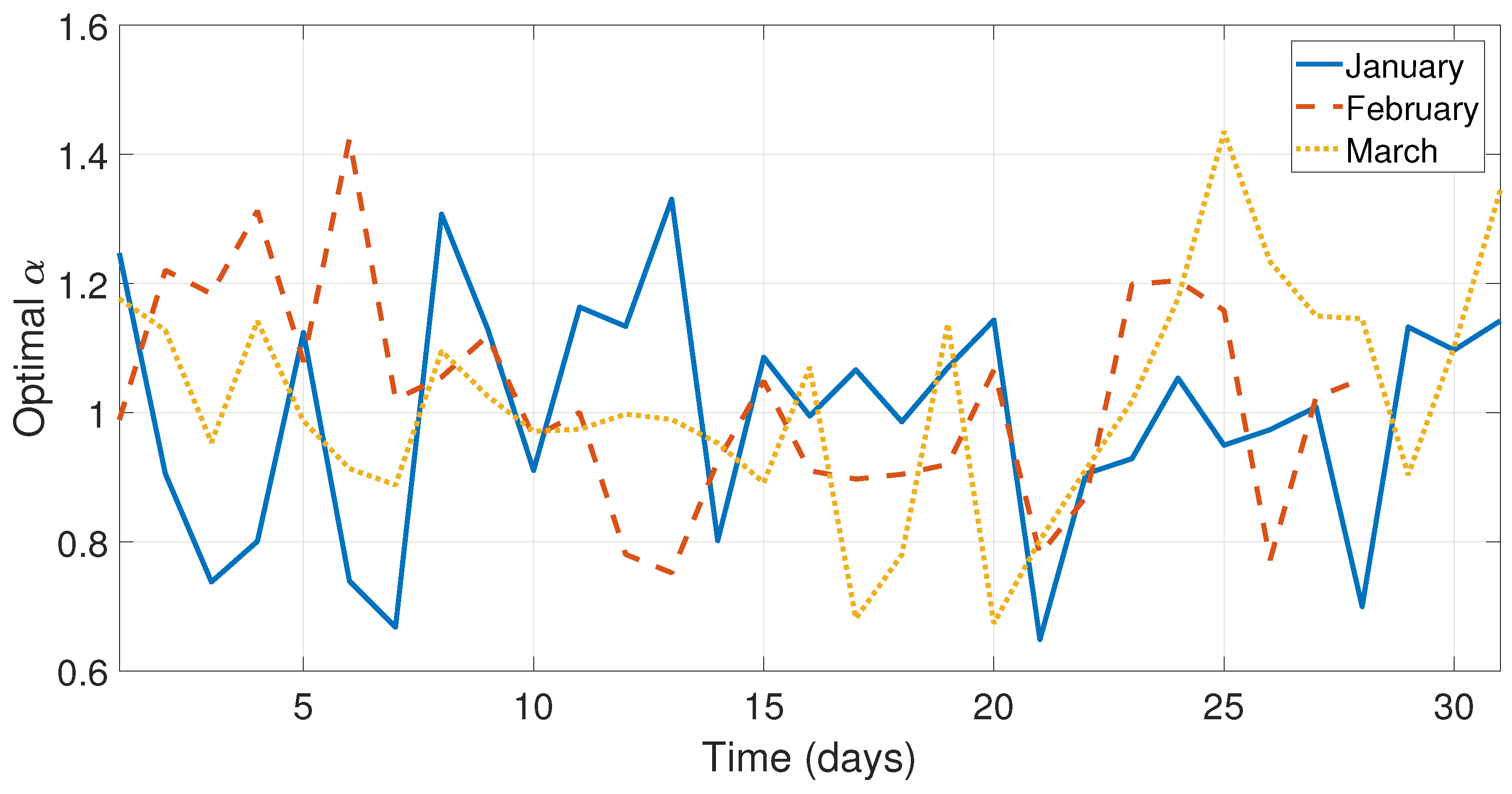
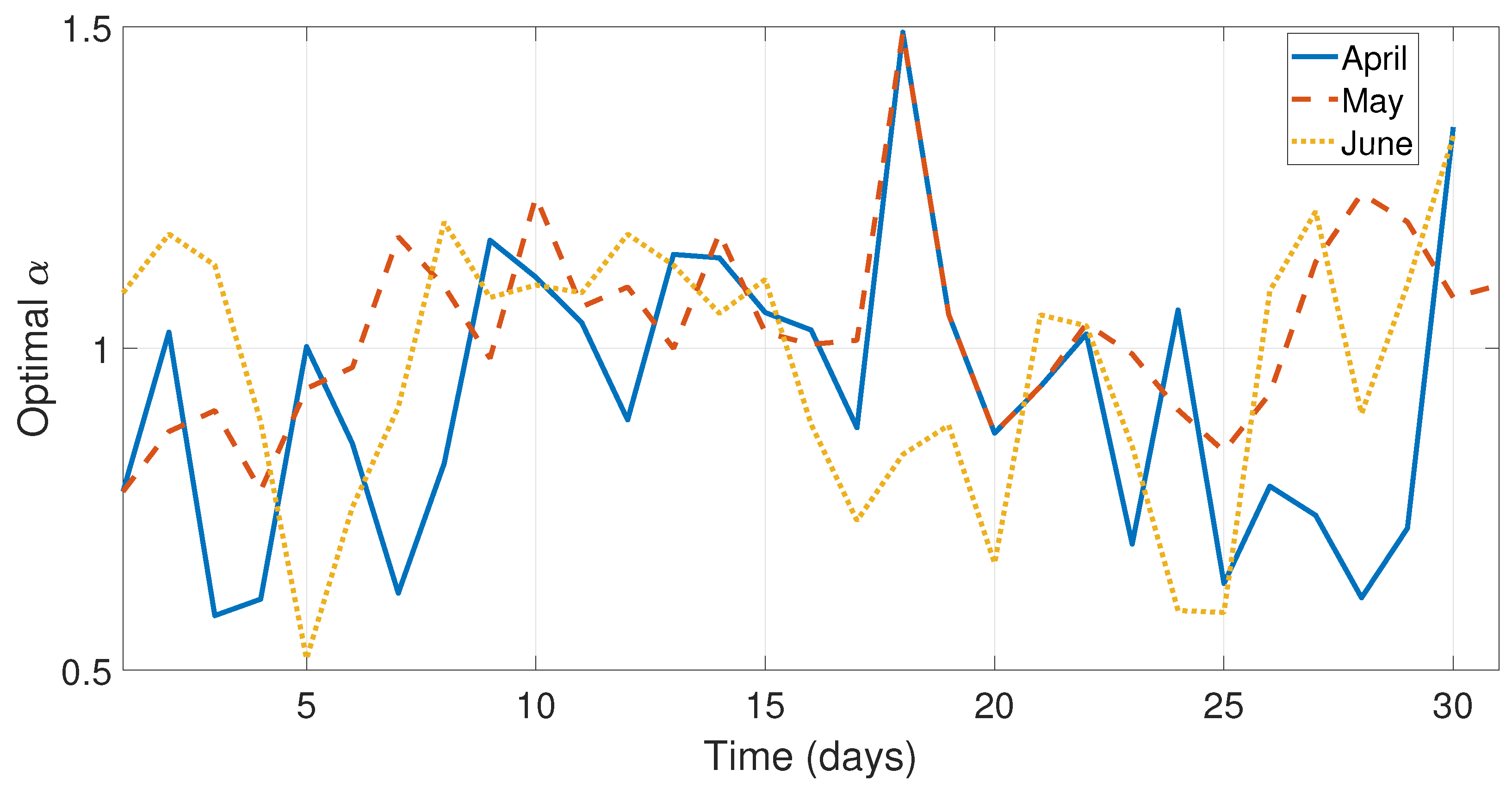
Figure 5 and
Figure 6 illustrate the optimal
behavior from the months January–June.
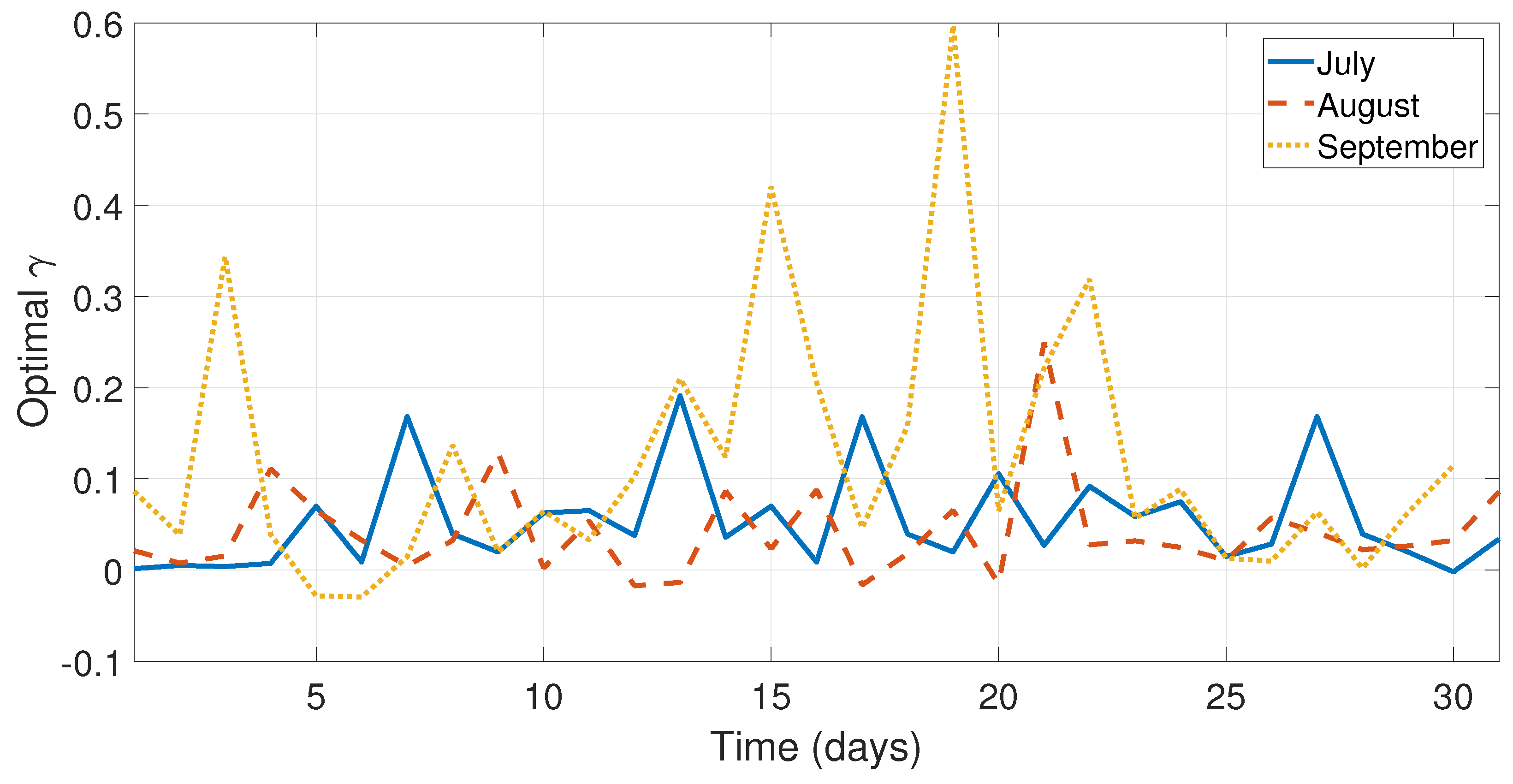
Figure 7 and
Figure 8 illustrate the optimal
and
calculated from the months July–September.
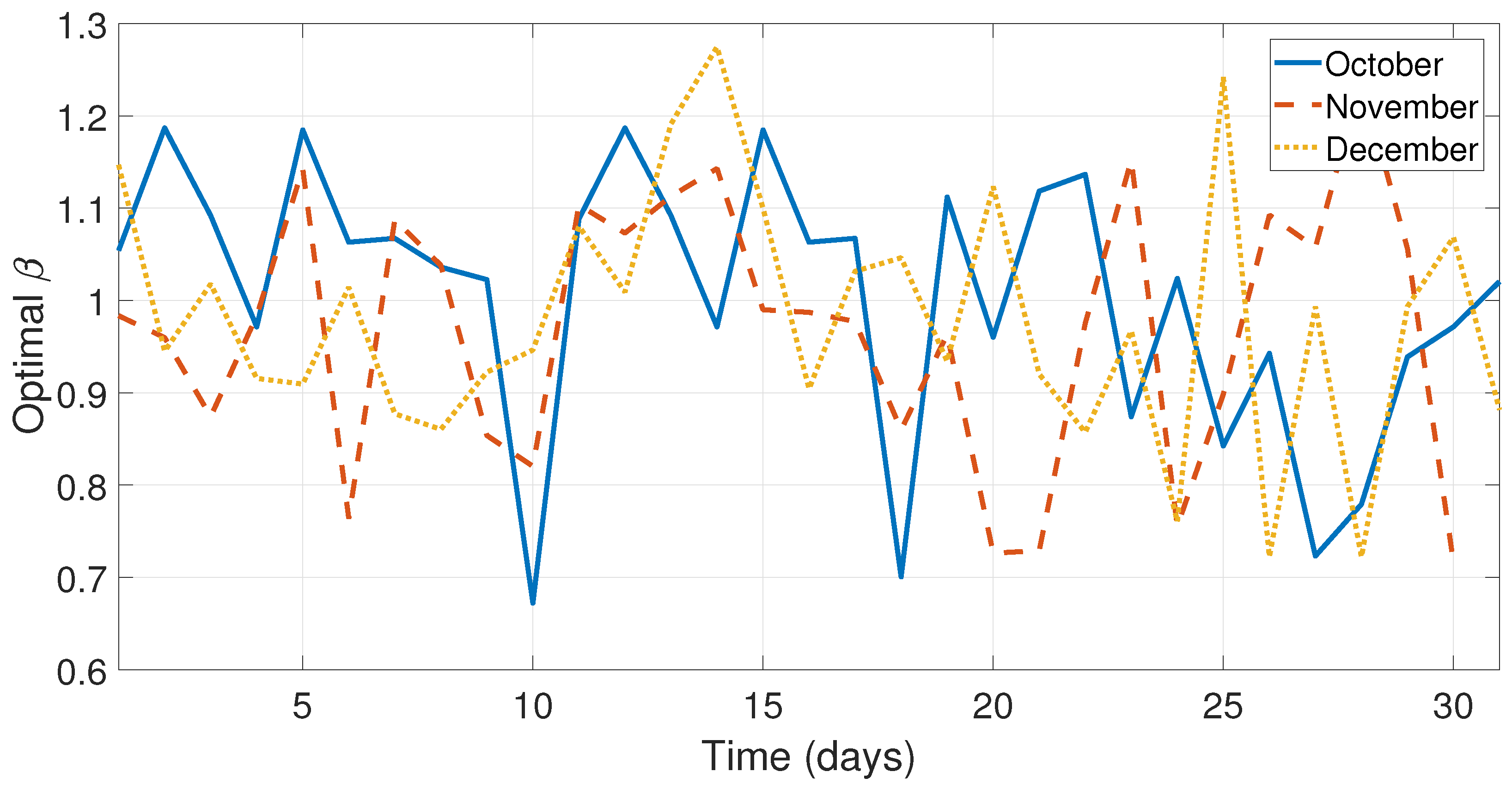
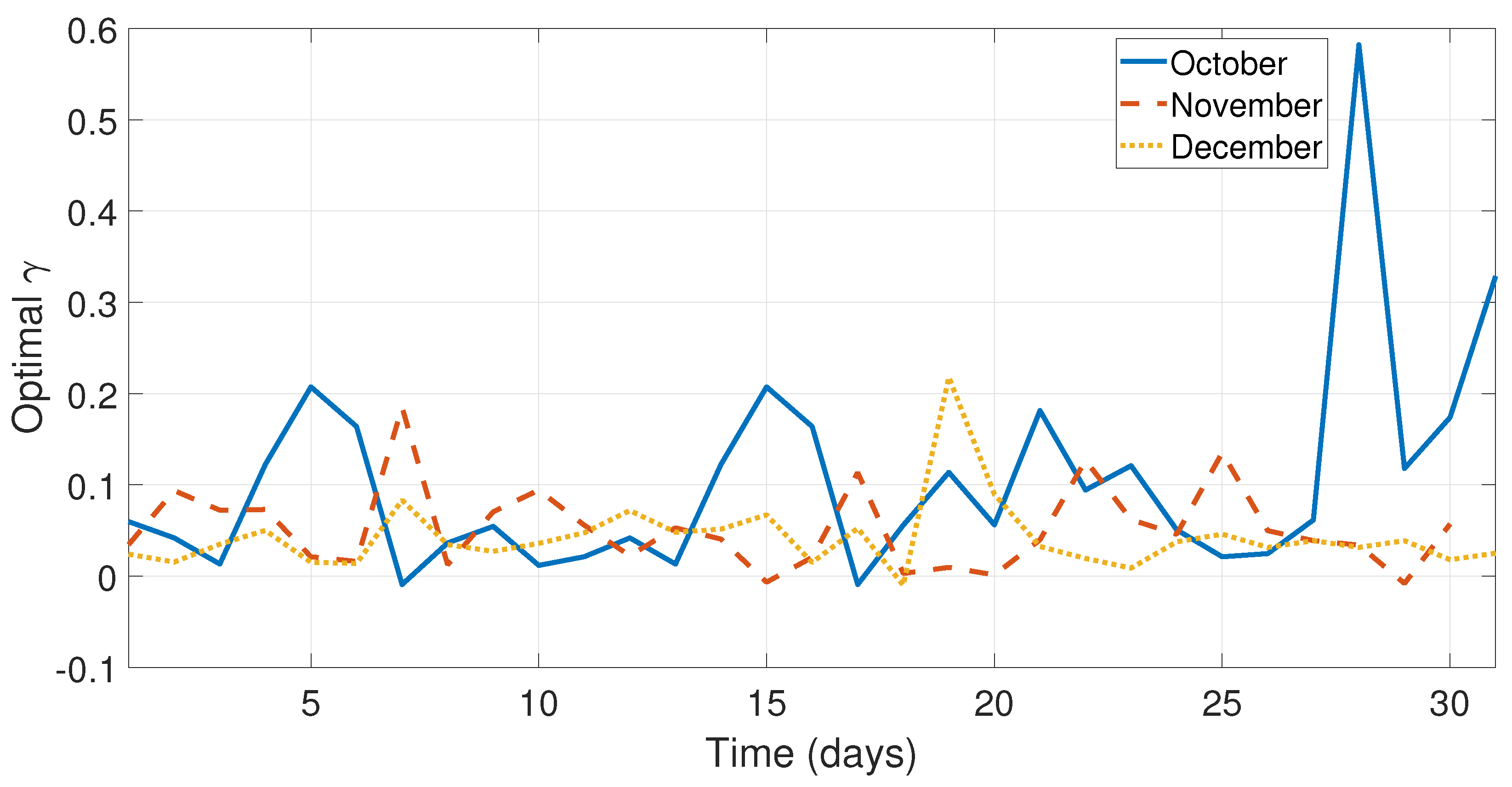
Figure 9 and
Figure 10 illustrate the optimal
and
behavior from the months October–December.
As can be seen in
Figure 5,
Figure 6 and
Figure 7 and
Figure 9, the values of the optimal constants
and
in some cases are greater than 1, which contrasts the theory of the classical SES and DES methods, since the values
and
are assumed to be between 0 and 1 [
19,
40]. Similarly, the value of the optimal constant
in some cases is lower than 1, when it is speculated that the value oscillates between 0 and 1 according to the classic DES method [
40], see
Figure 8 and
Figure 10.
With the values of the optimal constants
,
, and
, the values of
,
, and
have been calculated for each month of the year, as presented in
Table 4.
Once the values of constants
,
, and
have been obtained, the methods developed in
Section 4 are applied.
5.1. Simulation
To evaluate and compare forecasting methods, the relative error
, the mean error
, the mean squared error
, the root mean square error
, and the coefficient of determination
have been calculated as follows:
where
is the mean of the month
As mentioned in
Section 3, the first forecasting methods for wind speed were based on the moving average method. Moreover, the recursive function
was analyzed. This is due to the similarity with the proposed method.
Table 5 reports the relative errors of the methods 2-SMA, 3-SMA, 2-DMA, 3-DMA, and the recursive function
.
As presented in
Table 5, the recursive function reports the best performance between these five methods. However, the methods developed in
Section 4 are implemented to reduce the relative and mean errors obtained by the recursive function.
With the values obtained for
,
,
,
,
, and
in the previous subsection, the methods developed in
Section 4 have been applied. After that, the forecasts with these methods have been analyzed and compared to the experimental data using different error flags. A summary of the results obtained from this analysis is presented in
Table 6,
Table 7,
Table 8,
Table 9 and
Table 10.
As can be seen in
Table 6, the ranges of the relative error were: 5.8199% to 10.4158% for SES method with
; 6.0283% to 11.1853% for DES method with
and
; 5.8835% to 10.5249% for SES method with
; and 7.3060% to 18.6109% for DES method with
and
. Furthermore, the average relative errors were 7.9510%, 8.4128%, 8.0213%, and 10.0586% for SES with
, DES with
and
, SES with
, and DES with
and
, respectively.
In the analysis of the relative error
, the method with the best performance for each month was the SES method with
except for February and June where the SES method with
obtained the smallest error, see
Table 4. However, the SES method with
generally performed the best as its average relative error was the lowest.
As presented in
Table 7, the ranges of the mean error were: 0.3524 m/s to 0.4241 m/s for SES method with
; 0.3620 m/s to 0.4506 m/s for DES method with
and
; 0.3564 m/s to 0.4249 m/s for SES method with
; and 0.4079 m/s to 1.0123 m/s for DES method with
and
. Moreover, the average mean errors were 0.3860 m/s, 0.4074 m/s, 0.3905 m/s, and 0.5062 m/s for SES with
, DES with
and
, SES with
, and DES with
and
, respectively.
In the analysis of mean error
, the method with the best performance for each month was the SES method with
, see
Table 6. Therefore, based on the mean error analysis, the SES method with
has the best performance.
In
Table 8 and
Table 9, the mean squared errors and the root mean squared errors are reported. The ranges of the mean squared error were: 0.2485 to 0.5009 for SES method with
; 0.2805 to 0.5511 for DES method with
and
; 0.2558 to 0.5046 for SES method with
; and 0.3455 to 11.2723 for DES method with
and
. Furthermore, the average mean squared errors were 0.3615, 0.4046, 0.3681, and 1.4478 for SES with
, DES with
and
, SES with
, and DES with
and
, respectively. The ranges of the root mean squared error were: 0.4985 m/s to 0.7077 m/s for SES method with
; 0.5296 m/s to 0.7423 m/s for DES method with
and
; 0.5058 m/s to 0.7423 m/s for SES method with
; and 0.5878 m/s to 3.3574 m/s for DES method with
and
. Moreover, the average root mean squared error were 0.5974 m/s, 0.6319 m/s, 0.6029 m/s, and 0.9555 m/s for SES with
, DES with
and
, SES with
, and DES with
and
, respectively.
Based on the analysis of mean squared error and the root mean squared error, the method with the best performance was the SES method with .
Table 10 reports the coefficients of determination. These values had the following ranges: 0.9132 to 0.9755 for SES method with
; 0.9081 to 0.9727 for DES method with
and
; 0.9117 to 9748 for SES method with
; and 0.4691 to 0.9621 for DES method with
and
. The average coefficients of determination were 0.9459, 0.9426, 0.9447, and 0.8882 for SES with
, DES with
and
, SES with
, and DES with
and
, respectively. In this case, the SES method with
has reported better performance.
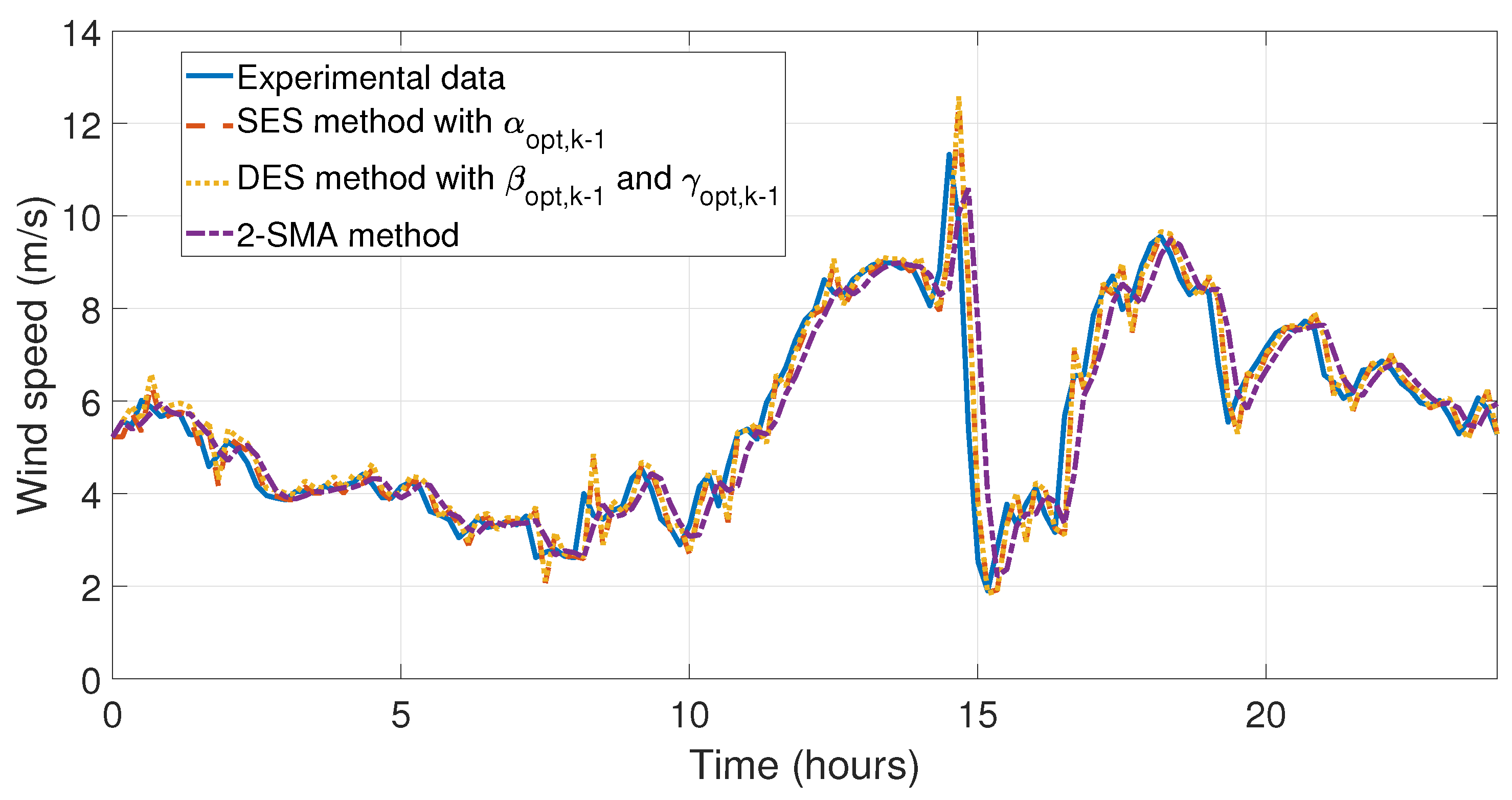
Once the analysis had been carried out, the simulations were carried out to be able to observe the behavior of the forecasting methods developed in this work. The simulations compared the SES with
, DES with
and
, SES with
, DES with
and
, and 2-SMA methods, which have shown the lowest relative and mean errors. In
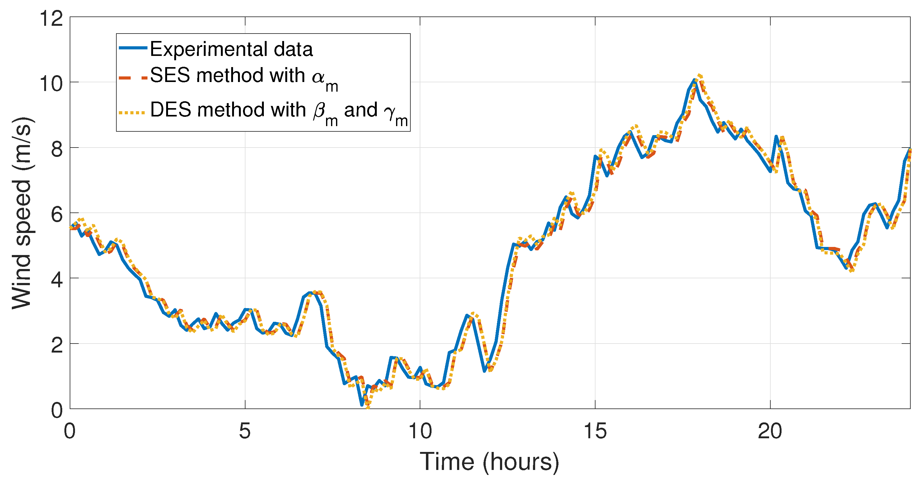
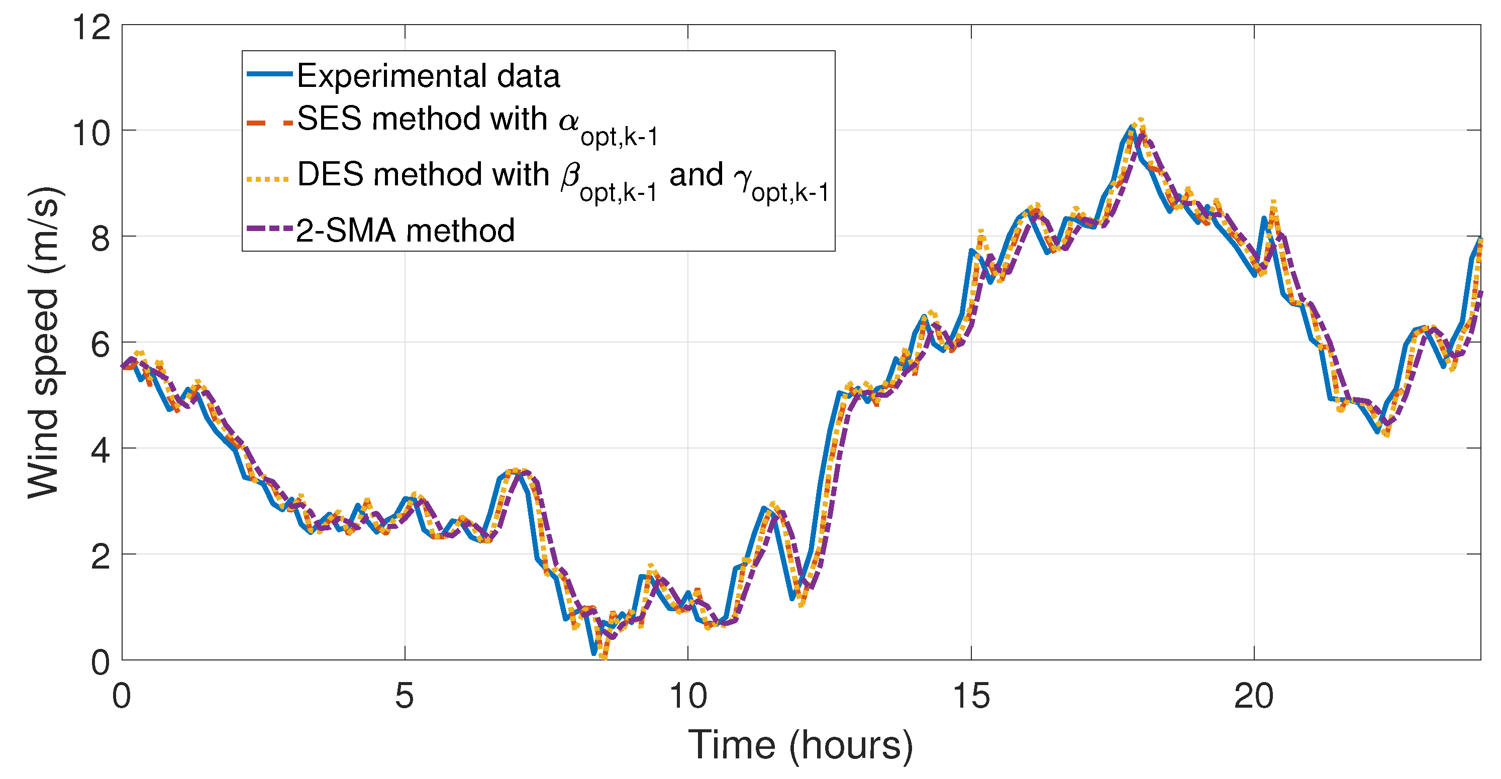
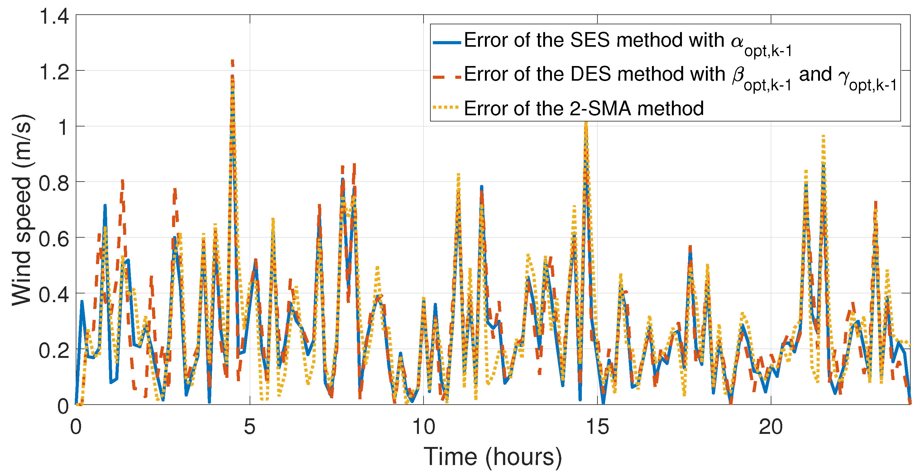
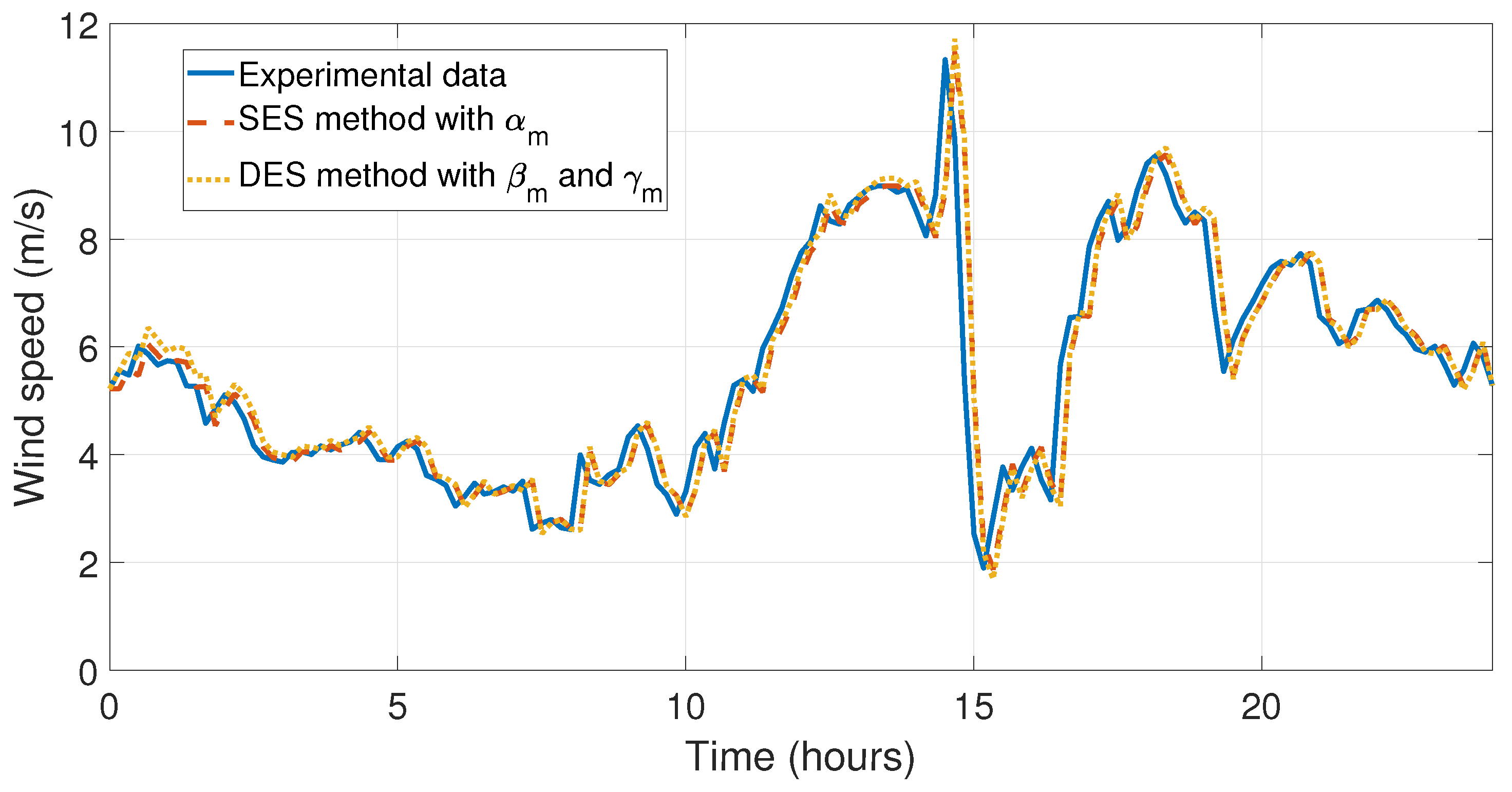
Figure 11 and
Figure 12 the behavior of the data taken on the first day of January and the simulations of the forecasting methods proposed in this work can be appreciated. In
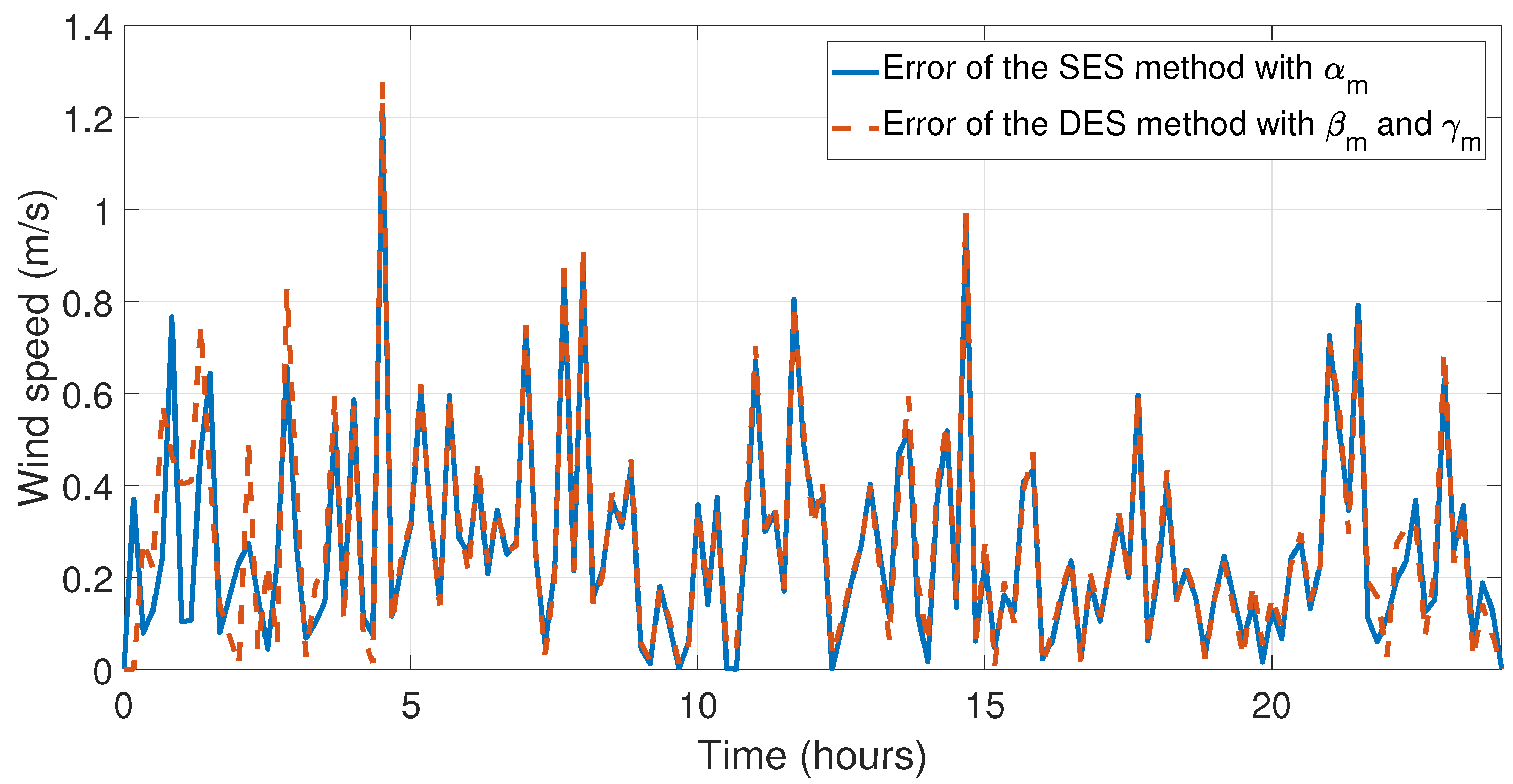
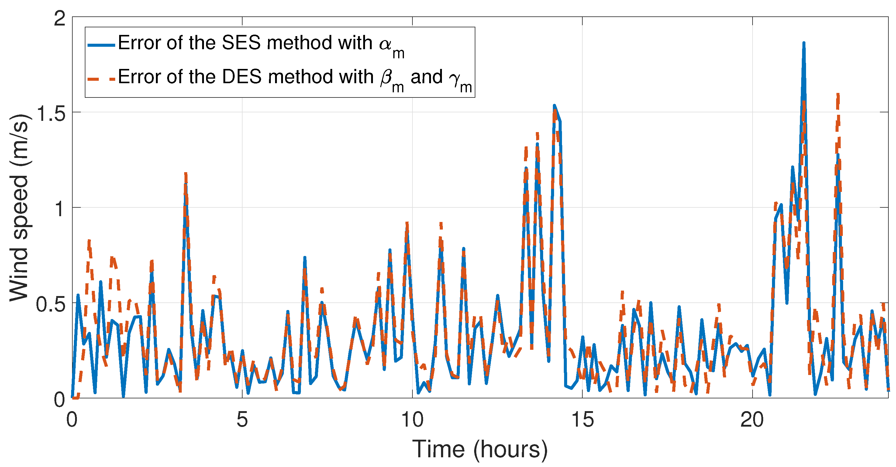
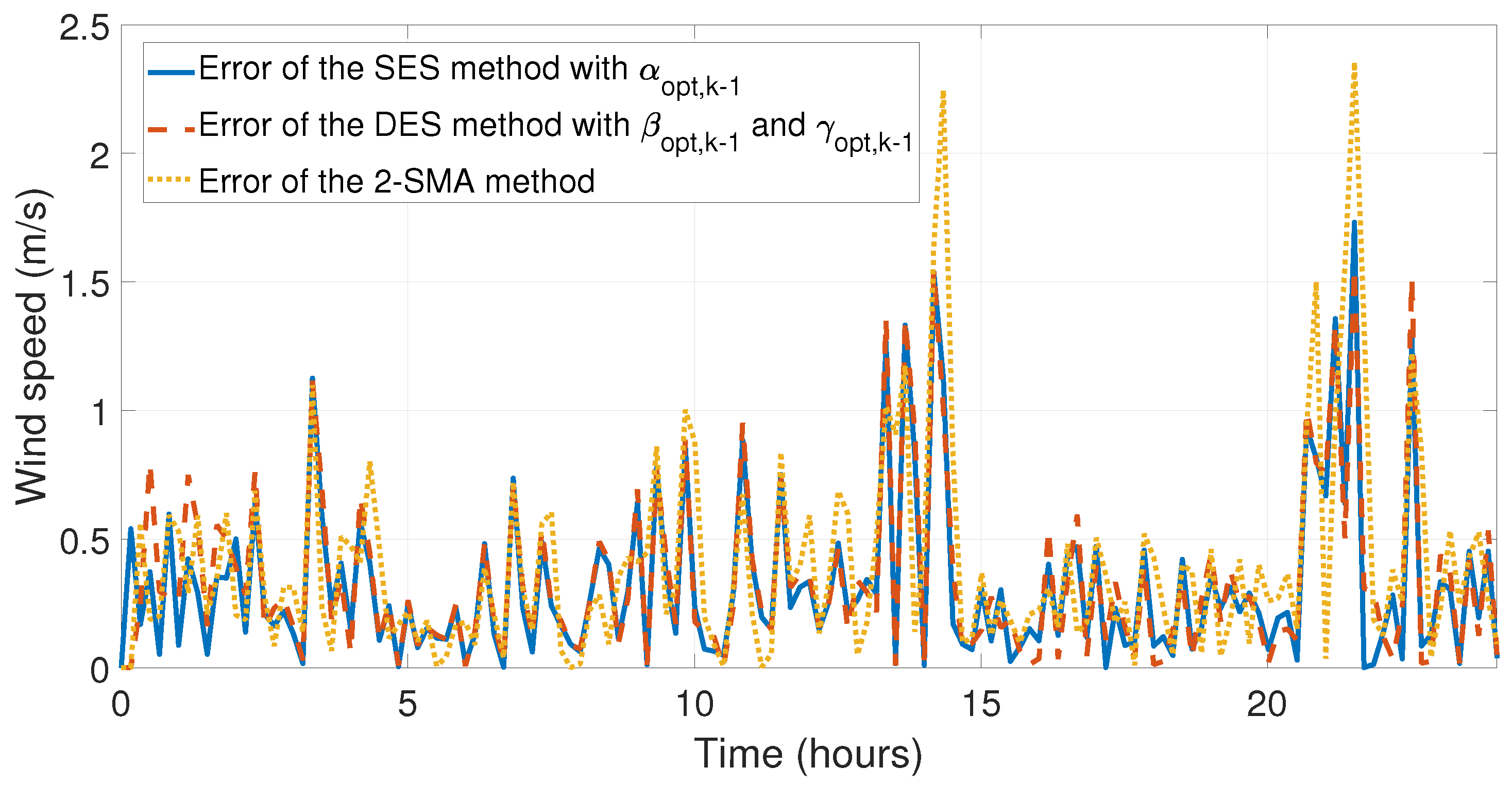
Figure 13 and
Figure 14, the errors between experimental data and the forecast for the first day of May have been illustrated, which is the month with the lowest relative errors (see
Table 6). The last four simulations illustrate the behavior and comparison of the forecasts with the highest relative and mean error, see
Table 6 and
Table 7. In
Figure 15 and
Figure 16, the behaviors of the data taken and the forecasts corresponding to the first day August have been shown, in this month the SES with
, DES with
and
, and 2-SMA methods incurred their largest relative error. Finally,
Figure 17 and
Figure 18 illustrate the behavior of the error of the comparison between experimental data and the forecasts for the first day of September, where the SES method with
and DES method with
and
obtained their largest relative error.
5.2. Discussion
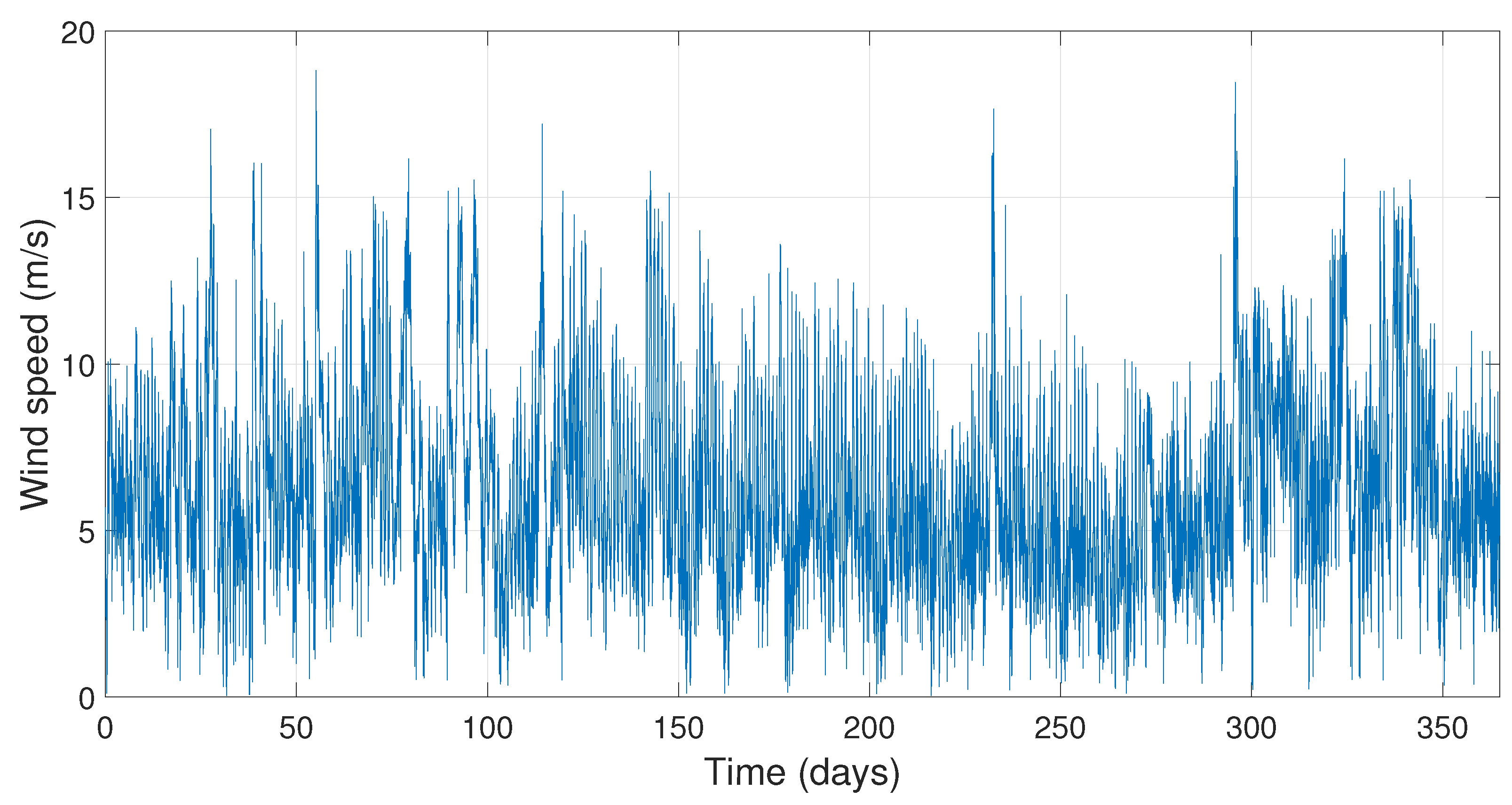
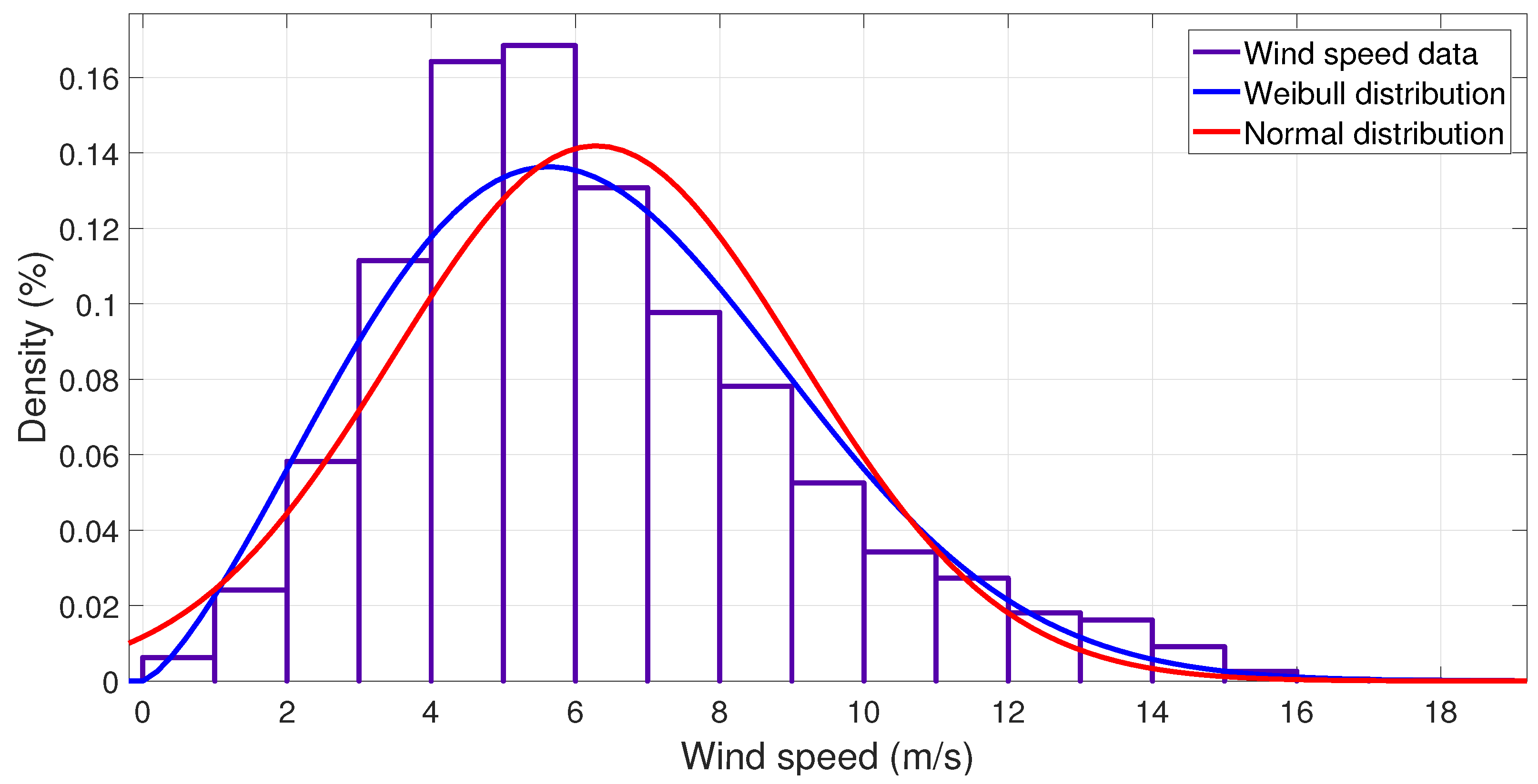
With the methods developed in this work, it is possible to obtain up to an average relative error %, an average mean error m/s, an average mean squared error , an average root mean square error m/s, and an average coefficient of determination , which indicate a high degree of accuracy of the proposed methods (i.e., due to the amount of experimental data used in this work, 52,560 wind speed data). Moreover, based on the analysis carried out, the SES method with has reported the best performance by having the lowest errors. Therefore, the developed method in this work is effective in forecasting wind speed data. However, the estimation of the model is not optimal, and errors between the experimental data and the model can be observed. Furthermore, the obtained errors are particularly noticeable in some months, which are complex to forecast according to the weather conditions. Thus, taking into account the weather conditions, it is possible to increase the reliability of this forecasting method.

 ,
, 


