Article

Using Self-Organizing Map Algorithm to Reveal Stabilities of Parameter Sensitivity Rankings in Microbial Kinetic Models: A Case for Microalgae

by
Dhan Lord B. Fortela
1,2,*,
Alyssa M. DeLattre
1,
Wayne W. Sharp
2,3,
Emmanuel D. Revellame
2,4 and
Mark E. Zappi
1,2
1
Department of Chemical Engineering, University of Louisiana, Lafayette, LA 70504, USA
2
Energy Institute of Louisiana, University of Louisiana, Lafayette, LA 70504, USA
3
Department of Civil Engineering, University of Louisiana, Lafayette, LA 70504, USA
4
Department of Industrial Technology, University of Louisiana, Lafayette, LA 70504, USA
*
Author to whom correspondence should be addressed.
Clean Technol. 2023, 5(1), 38-50; https://doi.org/10.3390/cleantechnol5010003
Submission received: 19 July 2022 / Revised: 17 December 2022 / Accepted: 22 December 2022 / Published: 26 December 2022

Abstract

:
Microalgae are multi-purpose microbial agents due to their capability to efficiently sequester carbon dioxide and produce valuable biomass such as protein and single-cell oils. Formulation and tuning of microalgae kinetics models can significantly contribute to the successful design and operation of microalgae reactors. This work aimed to demonstrate the capability of self-organizing map (SOM) algorithm to elucidate the patterns of parameter rankings in microalgae models subject to stochastic variations of input forcing functions–bioprocess influent component concentration levels. These stochastic variations were implemented on a modeled chemostat with a deterministic microalgae kinetic model consists of ten time-dependent variables and eighteen model parameters. The methodology consists of two major stages: (1) global sensitivity analysis (GSA) on the importance of model parameters with stochastic sampling of bioreactor influent component concentrations, and (2) training of self-organizing maps on the datasets of model parameter rankings derived from the GSA indices. Results reveal that functional principal components analysis can project at least 99% of the time-dependent dynamic patterns of the model variables on B-splines basis functions. The component planes for hexagonal lattice SOMs reveal that the sensitivity rankings some parameters in the algae model tested can be stable over a wide range of variations in the levels of influent component concentrations. Therefore, SOM can be used to reveal the trends in multi-dimensional data arrays arising from the implementation of GSA of kinetic models under stochastic perturbation of input forcing functions.

Graphical Abstract

1. Introduction

Some species of microalgae are multi-purpose microbial agents due to their capability to efficiently sequester CO2 and produce valuable biomass such as protein and single-cell oils. Microalgae can sequester CO2 at a rate of maximum of 2.35 GtCO2 can be sequestrated in 100,000 km2 culture area, accounting for 8.01–5.31% of global CO2 emission reductions in 2020 [1], which is the reason for considering it as potential CO2-to-O2 conversion platform for future space-based human settlements [2]. The protein and single-cell oils from microalgae have been demonstrated as alternative energy source such as biodiesel [3] and food such as human or animal feed protein supplement [4]. An important consideration for the successful design and operation of microalgae processing systems is a sound growth kinetics model used for growth analysis and process design [5]. In addition to the mathematical structure, parameter tuning of microalgae kinetics models can significantly contribute to the design and operation of microalgae reactors [6].
With the increasing capabilities in computational tasks in terms of hardware and software, mathematical models of dynamical systems have been finding important roles in system analysis. Among these are the kinetic models of microbial processes such as those of microalgae [7,8]. The literature for modelling microalgae growth still lacks comprehensive models combining the effects of various factors [8]. The growth dynamics of microbial systems is commonly modeled as a set of ordinary differential equations (ODEs). Inherent to these kinetic models and the actual microbial system being modelled are the effects of forcing functions such as the concentrations of influent components going into the cultivation space, i.e., bioreactor or bioprocess. These forcing functions have been empirically shown to be significantly influencing microbial system dynamics [9]. The area of wastewater treatment for example has seen a surge of various kinetic models depending on the type of feed wastewater [10,11]. Consequently, these observations warrant the investigation on the implications of variations of influent components concentrations on the dynamics of a microbial system being cultivated in a bioreactor or bioprocess. In modelling terms, the effects of various factors and processes in microbial dynamics are captured through the model parameters. This work aimed that demonstrating that the rankings of parameter sensitivities in microbial kinetics can be simply mapped out through the machine learning algorithm of self-organizing map (SOM). This mapping of parameter sensitivity rankings shall aid in revealing whether or not such parameter rankings can be stable across a wide range of variations in the concentrations of influent components into a continuously operated microbial bioprocess. Among many variables that have been accounted in microbial kinetic models, the component concentrations in the liquid-phase were selected because they are the common variables in fundamental model components, e.g., power law form that is fundamental in reaction kinetics starts with concentration variables main factors [9].
The importance of model parameters in affecting the simulated dynamics of a microbial kinetics can be computationally evaluated using global sensitivity analysis (GSA) techniques. Among the many GSA techniques, the Morris screening technique has been shown to be computationally effective due to minimal number of simulations needed to the calculate the sensitivity indices [12]. An improvement in implementing Morris GSA on microbial kinetics is the integration of functional principal component analysis (fPCA) of the time-series datasets of the response variables [13,14]. In this GSA-fPCA methodology [15], the fPCA projects the time-series datasets onto basis functions, e.g., B-splines, Fourier Series, and this projection allows for the calculation of basis function coefficients, which consequently reflect the dynamics of the model response variables. An efficient projection onto basis function coefficients, which are also called scores, provides a holistic measure of the elementary effects of perturbing the model parameters in the Morris GSA. The aggregated GSA indices can then be used to rank the model parameters for various purposes including model calibration and model simplification.
Computationally evaluating the effects of variations of influent components concentrations on the dynamics of a microbial system poses a challenge of dimensionality. That is, the random samples of the influent component concentrations and the calculated GSA indices at each simulation stance all combined together produces an array of data that cannot be simply evaluated on an apparent 2D or 3D space. One technique that is very effective in elucidating patterns in high-dimensional datasets is the machine learning technique of SOM [16,17]. Since its invention, SOM has been applied to various fields and problems [18], e.g., economic stability analysis, social interactions, fault diagnosis, adaptive authentication systems, facial emotions quantitation, fall detection in smart phones, and atmospheric sciences. A survey of the literature done for this work found that SOM has not been implemented as a computational tool to reveal the patterns of model parameter sensitivities in microbial kinetics. Hence, this work should provide an expanded area of application of the SOM algorithm. Further, this demonstration should lay down a numerical technique to comprehensively evaluate sensitivities of parameters in microbial kinetic models.

2. Methodology

The methodology consists of two major stages: (1) global sensitivity analysis (GSA) on the importance of model parameters while perturbing the levels of bioreactor influent component concentrations, and (2) training of self-organizing maps on the datasets of model parameter rankings derived from the GSA indices. A graphical summary of the methodology is shown in Figure 1.

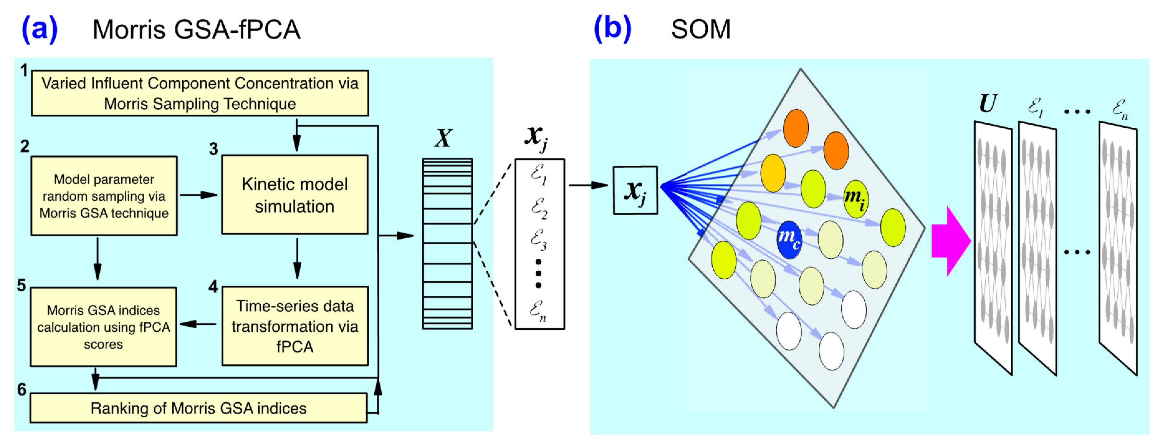
2.1. Algae Model Parameter Sensitivity Analysis

The first stage of GSA-fPCA is based on previous works of performing GSA on microbial kinetic models such as anaerobic digestion [14], and aerobic activated sludge [13]. The unique feature of the GSA-fPCA in this work is the integration of stochastic sampling of influent component concentrations (Figure 1a) through Morris technique [12] to generate simulated variations in the influent to the algae reactor. This stochastic sampling step represents the randomness of influent concentrations. The microalgae model used in this work was based on the kinetic model formulated by Solimeno, Samsó [5]. See Supplementary Materials for the detailed equations of the model used. A chemostat was assumed for algae cultivation: inflow and outflow liquid rates = 75-L/day, liquid-phase volume = 450-L, gas-phase volume = 60-L, solids retention time (SRT) = hydraulic retention time (HRT) = 6 days [7,19]. The algae CSTR influent component concentrations were randomly generated via Morris sampling technique from a sampling set with set upper-bounds and lower-bounds based on typical empirical values (see Table 1). There are 10 model response variables, and the Morris technique sampled r y [ k y + 1 ] = 220 combinations of the influent component concentration levels, where k y = 10 is the number of model response variables, and r y = 20 is the number of randomly sampled level increments in each variable. The algae model parameters evaluated in the sensitivity analysis step are summarized in Table 2, in which the sampling bounds for the model parameters are ± 30 % of the nominal values reported by Solimeno, Samsó [5]. Note that the actual temperature of the algae system, T a c t , and the irradiance intensity, I i r r a d , were treated as parameters in the context of GSA even though these can be system variables particularly when an algae cultivation process is exposed to the external environment with weather and seasonal variations [7]. This is a simplification of the computational analysis, but these may also be practically realized when the algae system is operated in enclosed controlled setup. The differential equations and the associated variable and parameter definitions for the algae model used in this work are summarized in the electronic Supplementary Document for this work (see Supplementary Materials section). The kinetic model integrated within the GSA-fPCA computational steps was coded in the programming language R-statistical software (see Supplementary Materials section to download the R-script). The magnitude of the sensitivity index μ * in the Morris GSA technique indicates the relative influence of a model parameter on a model response variable [12] (see Appendix A for the equations involved in calculating μ * ). Hence, a ranking of μ * levels for a set of model parameters under GSA indicates the order of importance of the parameters in uncertainty analysis and model parameter calibration [13,14]. The interaction effect of a model parameter can be measured using the interaction index σ in the Morris GSA. High levels of σ means the parameter sensitivity is highly confounded by other model parameters. The formula for both μ * and σ are shown in the Appendix A section as Equations (A4) and (A5), respectively.

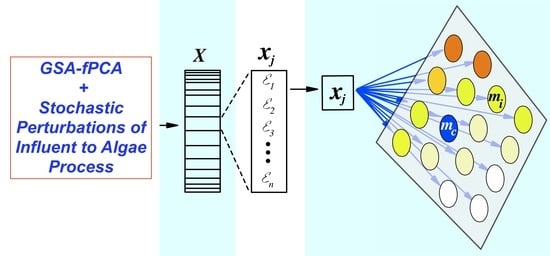
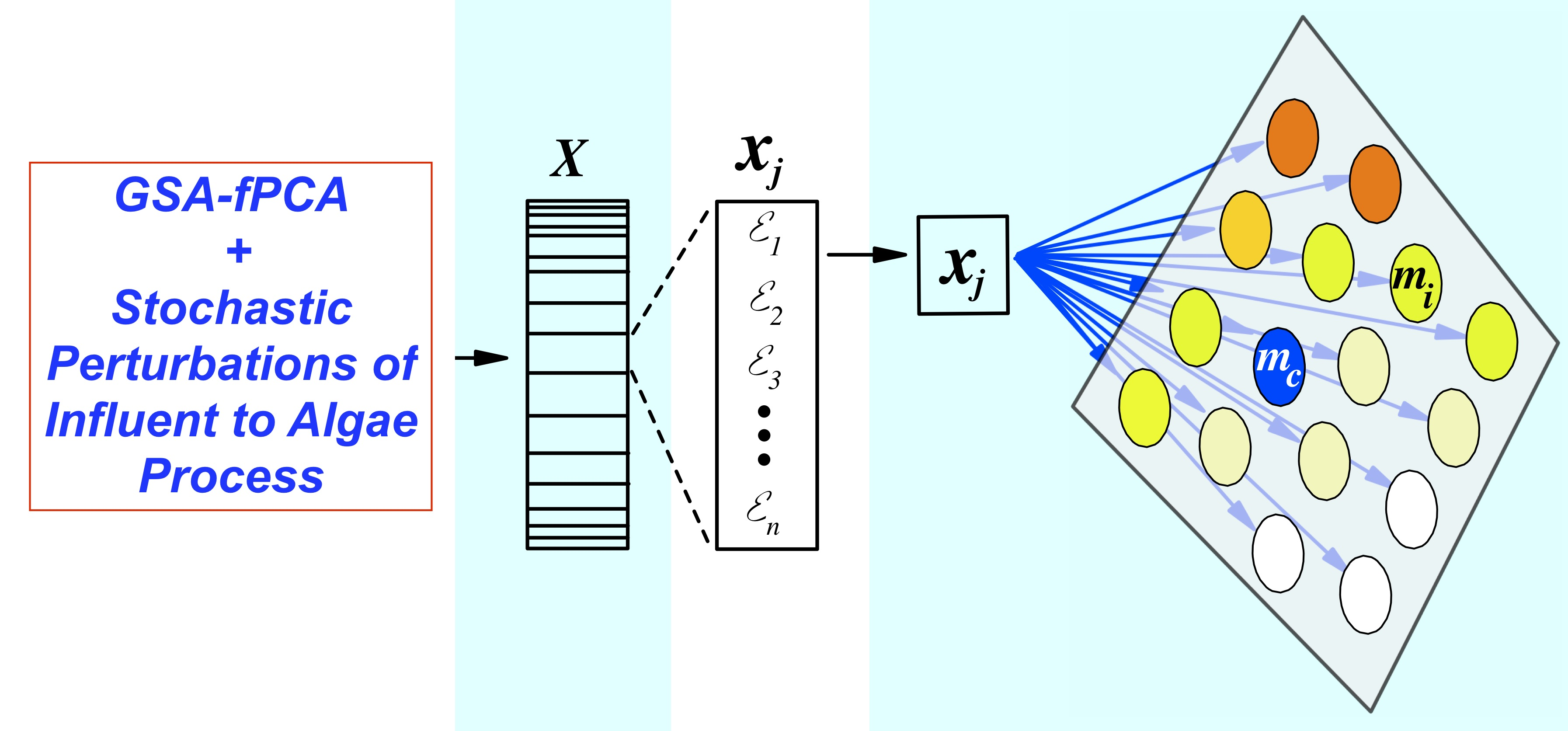
2.2. SOM Training on Parameter Sensitivity Index and Ranking

After all model simulations and parameter sensitivity index calculations were completed, the generated datasets were used to train SOM (Figure 1b). The datasets were of two matrices (1) the randomly sampled 10 variables for the influent component concentrations together with the μ * of PC1 of the S O 2 variable on the 18 model parameters; (2) the randomly sampled 10 variables for the influent component concentrations together with the ranking of the 18 model parameters based on the μ * of PC1 of the S O 2 variable. The structure of SOM can be varied and there are no current established rules to guide the specification of the map architecture. Nonetheless, results of some works that implemented SOM provide basis of map design. It was shown that the patterns elucidated by rectangular SOMs may not be so different from those of cylindrical SOMs [20]. Hence, this study uses rectangular SOM. The number of neurons or size of a SOM may be estimated using this proposed formula: 5 S [21], where n is the number of variables used for SOM training, i.e., 1 , , n , and S is the number of samples, which is equal to the number of simulation runs generated during the Morris sampling of the influent component concentration levels. Hence, n = 28 , S = 220 , and 5 S × n = 393 number of neurons. Another component of a rectangular SOM architecture is the ratio of length to width, which also does not have a set rule, but it is suggested that the map should not be a square map for proper orientation and stabilization of the learning process [17]. So, a SOM length of 40 neurons and width of 10 neurons was used, i.e., a total of 40 × 10 = 400 neurons. Lastly, the arrangement of the neurons on the map is commonly specified as hexagonal lattice structure because it does not favor horizontal and vertical directions [17]. All SOM calculations were implemented through MATLAB (MathWorks®) using the public-domain add-in SOM Toolbox version 2.0 [17,21,22] (see Supplementary Materials section for the accompanying program code).

3. Results

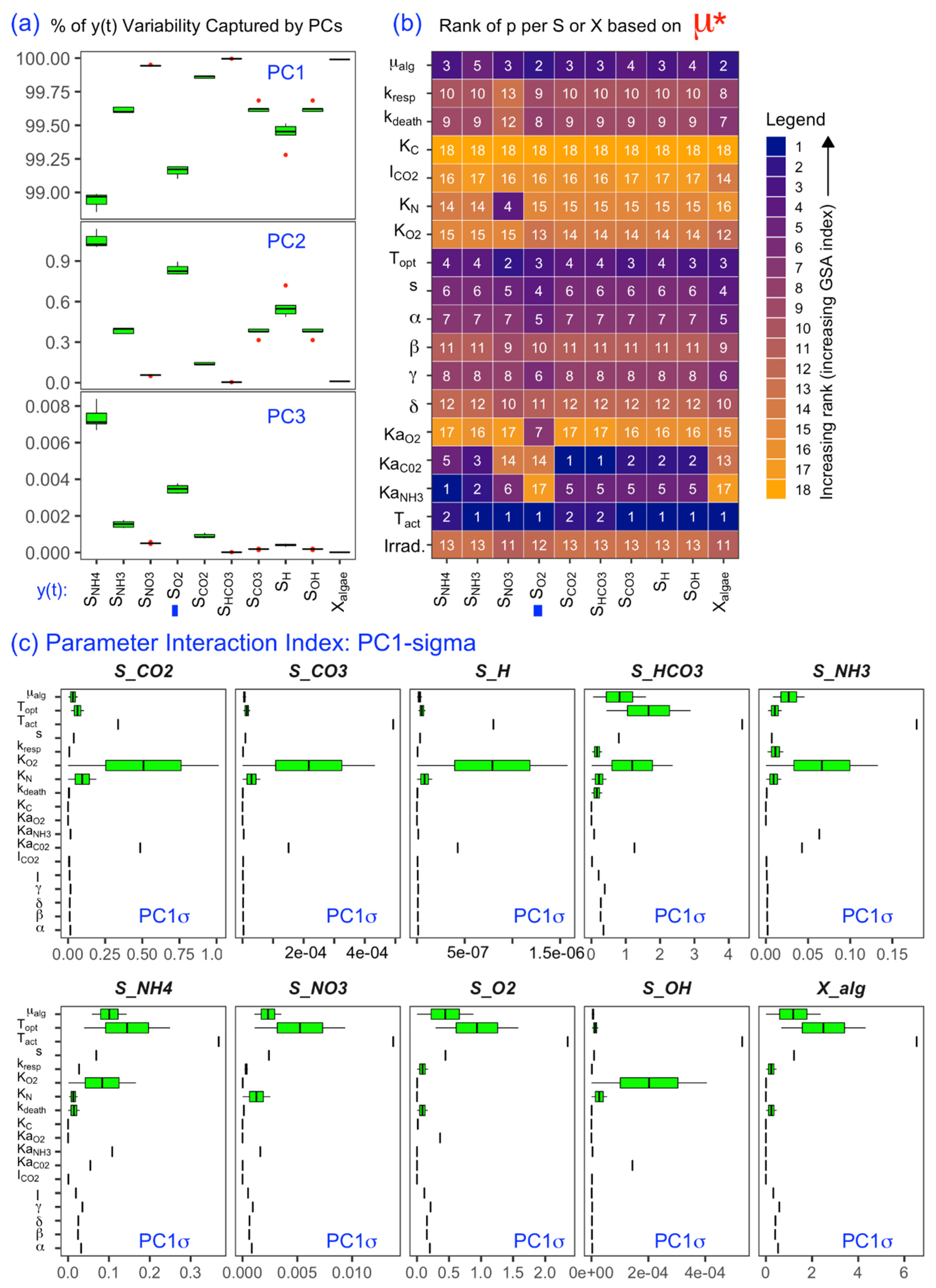
3.1. Effectiveness of GSA-fPCA in Calculating the Sensitivity Indices for Model Parameters Ranking

The performance of the GSA-fPCA methodology in calculating for the Morris sensitivity indices must be evaluated prior to the use of the indices for SOM. Figure 2a shows the percentages of model response variabilities captured by the first three PCs. It can be seen that the PC1 captures at least 99% of the time-series response dynamics across all the model variables. PC2 and PC3 captures the remaining small percentages, i.e., less than 1% (Figure 2a). This indicates that the associated scores of PC1 in all the model variables are good representations of the dynamics relative to the mean curve of the time-series dataset of each variable. Hence, the scores solely of PC1 are sufficient in calculating representative values of the GSA indices for each model parameter. Relatively high values of Morris index μ * of a model parameter mean high sensitivity of a model variable to that particular parameter. The ranking of the model parameters based on μ * of PC1 basis function are shown in Figure 2b with rank 1 having the highest value of μ * and rank 18 having the lowest. The pattern of these rankings indicate that the relative importance of the model parameters are almost consistently maintained across the model response variables. Few parameters can switch sensitivity levels drastically from one response variable to another such as K N , K a O 2 , K a C O 2 , and K a N H 3 . On the other hand, model variables are consistently very sensitive to T a c t , μ a l g , and T o p t . The temperature T a c t was found to be significantly influencing the growth of microalgae [7,23]. With the significant effect of temperature, various model forms have been evaluated to better capture its dynamics with microalgae growth [8].
An aspect parameter sensitivity that must also be considered is the interaction effect of the parameters. If parameter interaction is high, then the confounding effect of sensitivity is also high. Figure 2c shows the levels of the Morris GSA parameter interaction index σ . It can be seen that some parameters have dominantly high interaction levels when sensitivity is evaluated against certain state variables. For example, parameter KO2 has high interaction levels when the sensitivity of state variables SCO2, SCO3, SH, SHCO3 and SNH3 are evaluated. Model parameter Topt has a dominant high level of interaction when the sensitivity of state variables SHCO3, SNH4, SNO3, SO2, and Xalg are evaluated. Model parameter Tact has a dominant high level of interaction when the sensitivity of all state variables are evaluated. The parameter μ a l g also has high interaction levels when the sensitivity of state variables SHCO3, SNH3, SNH4, SNO3, SO2, and Xalg are evaluated. The other model parameters have low to moderate interaction index level; hence, these are the parameters that have low confounding effect in terms of the sensitivity of the state variables.

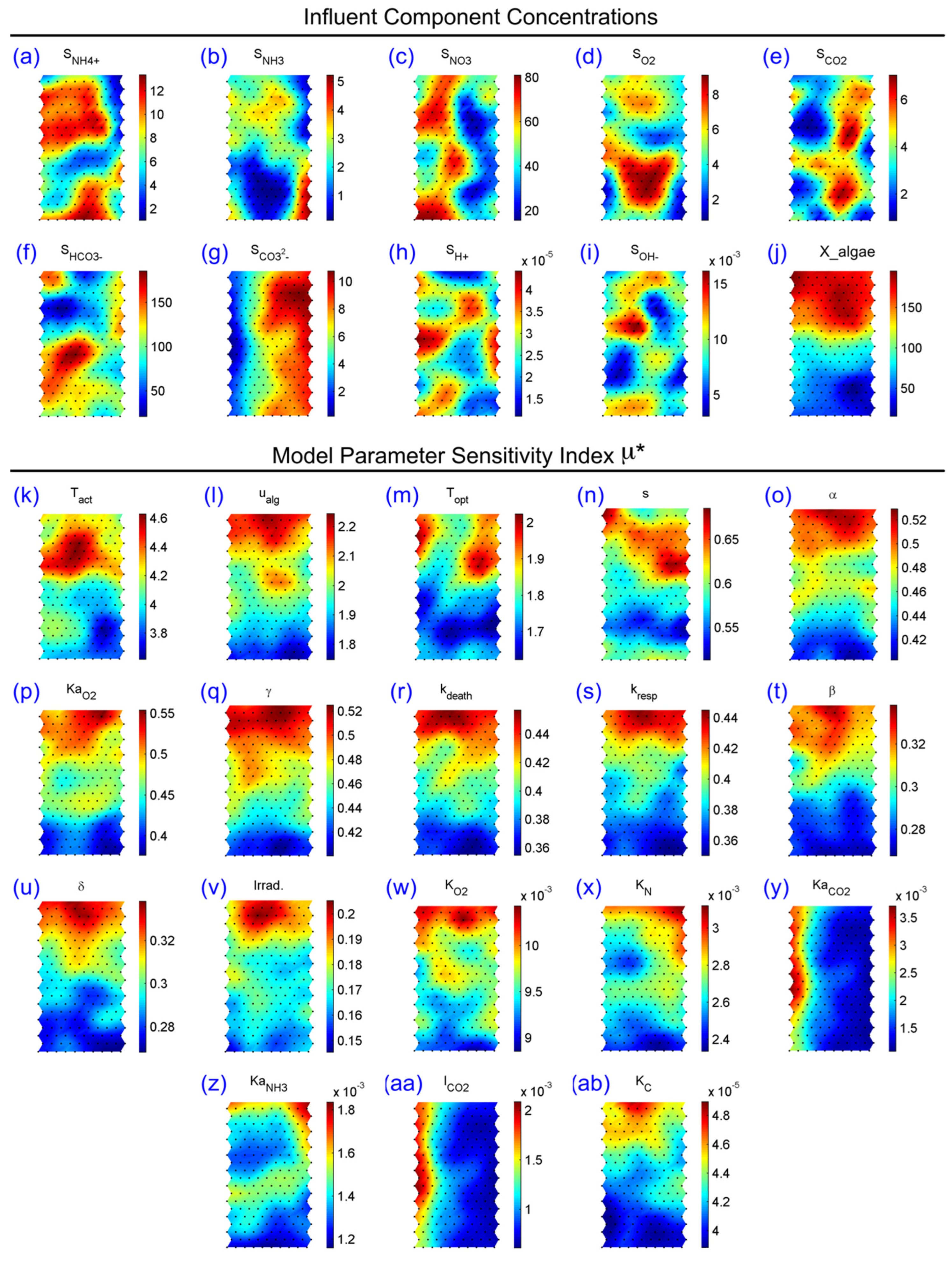
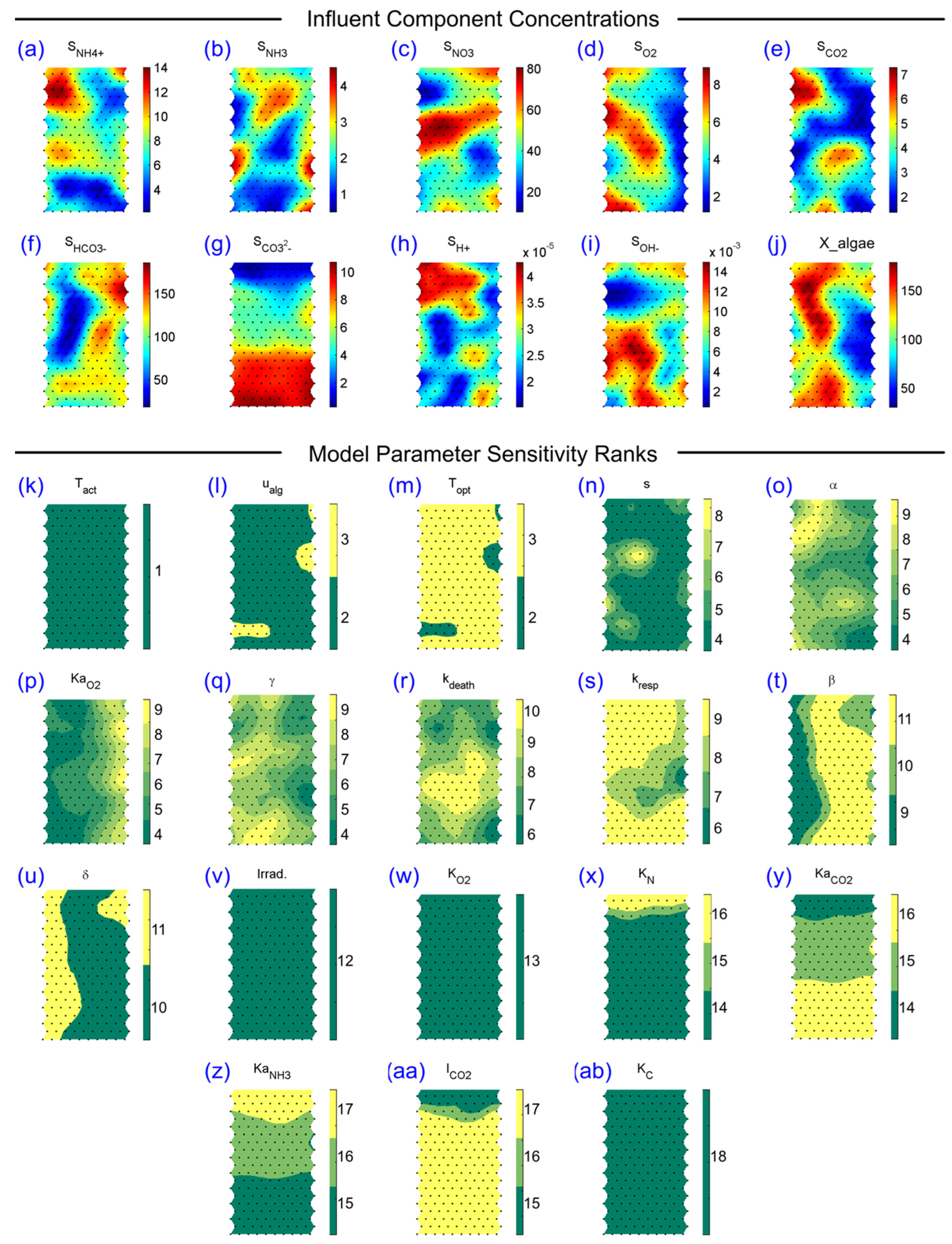
3.2. SOM Component Plane Projection of the Morris Sensitivity Index and Parameter Ranks

The model response variable S O 2 was selected for the demonstration of implementing SOM to elucidate patterns on the sensitivity indices and model parameter ranks. From the trained SOM, the useful analysis tools are the component planes, which show the mapping the various attributes. These mappings make the comparison of the variable patterns visually comprehensible. Figure 3 shows the component planes for the Morris sensitivity index μ * from PC1 of the S O 2 variable together with the randomly varied levels of the influent component concentrations. Figure 4 shows the component planes of model parameter ranks derived from the Morris sensitivity index μ * from PC1 of the S O 2 variable together with the randomly varied levels of the influent component concentrations. These graphical results suggest that some model parameters maintain dominant influence on the model response while some parameters have wide ranges of ranking levels. The parameters that have stable ranking level(s) are T a c t at rank 1,   μ a l g at ranks 2 and 3, T o p t at ranks 2 and 3, δ at ranks 10 and 11, I i r r a d at rank 12, K O 2 at rank 13, and K C at rank 18 (Figure 4).
The model parameters that have wide ranges of ranking levels are s at ranks 4 to 8, α at ranks 4 to 9, K a O 2 at ranks 4 to 9, γ at ranks 4 to 9, k d e a t h at ranks 6 to 10, k r e s p at ranks 6 to 9, β at ranks 9 to 11, K N at ranks 14 to 16, K a C O 2 at ranks 14 to 16, K a N H 3 at ranks 15 to 17, and I C O 2 at ranks 15 to 17 (Figure 4).

4. Discussion

Inherent to the use of time-dependent dynamical models such as microbial kinetic models are the problems on parameter calibration and model simplification [24]. A key step in solving both problems involves determination of the sensitivities of model parameters. In complex model forms such as the one used in this work [5], numerical procedures become necessary to perform GSA that estimates the parameter sensitivities. Model simplification for microbial systems has been gaining interest due to the need to compromise between model applications such as control theory, and availability or capability to collect empirical data for model calibration. Several computational techniques for GSA have already been successfully demonstrated in various GSA problems. Recent studies started focusing on the integration of these GSA techniques in systematic approaches for model calibration and validation [24]. Based on literature survey, this study is the first attempt to show a comprehensive approach to perform GSA on time-dependent microbial kinetic models subject to stochastic variations in the influent component concentrations, and this is accomplished through the integration of SOM for mapping of the sensitivity indices.
Unlike the works in anaerobic and aerobic wastewater treatment models [10,13,14], GSA for model simplification of microalgae models has not yet received much attention even though their structures are similar to the former. The parameter sensitivity patterns by SOMs in Figure 3 and Figure 4 warrant emphasis on some model parameters. Temperature effects such as the actual reactor temperature T a c t (rank 1) and the nominal optimum temperature T o p t (rank 2,3) that are both highly sensitive parameters (Figure 4) are known to have significant effects on microalgae dynamics [8]. It must be reiterated that temperature is mostly modeled as a system variable, and its strength of influence on microalgae dynamics were found next to dissolved nutrients [8,23]. These results confirm the findings of previous works that measured and modeled the effects of temperature on microalgae growth [23,25]. Even though its sensitivity was ranked average, light intensity I i r r a d (rank 12 in Figure 4) was found by previous works as a significant factor [23] next to temperature and dissolved nutrients. Light intensity has been commonly studied while the effect of light wavelength has only few published works [8]. There are debates on whether I i r r a d should be mathematically coupled with T a c t as their interdependency was found significant in some instances [25]. It has been suggested, however, that T a c t and I i r r a d should be uncoupled to eliminate complexities in the mathematics that may lead to overfitting [25]. The model by Solimeno, Samsó [5] used in this work maintains this uncoupling approach; hence the multiplication of the functions separately containing T a c t and I i r r a d (see Supplementary Materials). The maximum growth rate of microalgae μ a l g (rank 2,3) appears in several rate expressions defining various processes. Its high ranking manifests the importance of this fundamental step in the microalgae dynamics [8]. Moreover, four groups of parameter ranking patterns may be deduced from the results of computational analysis (Figure 3 and Figure 4): (1) high and stable rank order, (2) high and unstable rank order, (3) low and stable rank order, and (4) low and unstable rank order. The grouping of parameters based on sensitivity ranking warrants the question of the cut-off criteria between groups. Such establishment of criteria are of significant value and being suggested for future works.
Several variables influence the dynamics of microalgae cultivation–influent component concentrations are just few variables that must be considered for process simulation, design, and operation [7]. The intent of this work is to lay down a base protocol for the computational analysis of model parameter sensitivities to these potential variable fluctuations of various forcing functions. Other variables that have been accounted in existing microalgae models are microalgae species, salinity, reactor geometry, geographic location, and weather data [7,8]. Accounting for potential effects of the variables in these aspects during GSA for model parameter analysis will result to large arrays of data. An analysis of parameter sensitivities in such multi-dimensional arrays may be efficiently accomplished through the implementation of SOM as demonstrated in this work.

5. Conclusions

The findings in this work reveal that the ranks of some model parameters in the algae model tested can be stable over a wide range of variations in the levels of influent component concentrations. This implies that the strengths of the mechanisms being modeled through these model parameters may not significantly vary with variations in the influent variations. Therefore, SOM can be used to reveal the trends in multi-dimensional data arrays arising from the implementation of GSA of kinetic models under stochastic perturbation of input forcing functions. A future perspective based on the results of this work is the evaluation of the potential benefits of the proposed protocol to variables other than the influent component concentration levels.

6. Recommendations

Future implementations of this method should consider algal models that incorporate as state variable the phosphate (P) concentration in a limited supply so the effects of P variations can be modeled. The model used in this work, which is the model developed by Solimeno, Samsó [5], assumed that P is at an abundant supply, hence, as not a limiting nutrient and not modeled as a state variable. Based on the literature of algae dynamics, the P concentration can be critical to algal growth. Finally, some of the model parameters such as Topt may be specified if the species of microalgae is known, hence eliminating these specified parameters from the sensitivity analysis.

Supplementary Materials

The following supporting information can be downloaded at: https://www.mdpi.com/article/10.3390/cleantechnol5010003/s1, Document 1: Algae model differential equations and parameters. A copy of this material is also available in the project GitHub repository: https://github.com/dhanfort/NASA-LURA-2019-dlbfortela/blob/d329b38b35acee60b37ef6367201476f3ad6651f/Appendix%201%20-%20Algae%20Model%20ODEs.pdf; Code File 1: R-script of the GSA-fPCA of the microalgae model. A copy of this material is also available in the project GitHub repository: https://github.com/dhanfort/NASA-LURA-2019-dlbfortela/blob/9c8947e336ccae6274241e352f662da241db6747/Appendix%205%20-%20ALGAE_GSA_FPCA_.R; Code File 2: MATLAB code for the SOM training. A copy of this material is also available in the project GitHub repository: https://github.com/dhanfort/NASA-LURA-2019-dlbfortela/blob/d9c12ed9ffb72e5f5f9d10a20ef3357a3276accf/SOM_base1_Matlab_SOM_FINALresults.m.

Author Contributions

Conceptualization, D.L.B.F. and A.M.D.; methodology, D.L.B.F. and A.M.D.; formal analysis, D.L.B.F., W.W.S., E.D.R. and M.E.Z.; resources, D.L.B.F., W.W.S., E.D.R. and M.E.Z.; data curation, D.L.B.F. and A.M.D.; writing—original draft preparation, D.L.B.F. and A.M.D.; writing—review and editing, D.L.B.F., W.W.S., E.D.R. and M.E.Z.; funding acquisition, D.L.B.F. and M.E.Z. All authors have read and agreed to the published version of the manuscript.

Funding

This research was funded by the Louisiana Space Grant Consortium (LaSPACE) with subaward number PO-0000105697 under the primary grant from National Aeronautics and Space Administration (NASA) with primary grant number NNX15AH82H; and by the NASA-EPSCoR through the Louisiana Board of Regents with grant number 80NSSC18M0062.

Institutional Review Board Statement

Not applicable.

Informed Consent Statement

Not applicable.

Data Availability Statement

The supporting information and data files used and created in this work are publicly available online via the GitHub repository of the project: https://github.com/dhanfort/NASA-LURA-2019-dlbfortela.git.

Acknowledgments

We are grateful to the students and staff of the Energy Institute of Louisiana (EIL) at the University of Louisiana at Lafayette, particularly to Sheila Holmes and William “Bill” Holmes for assistance in project implementation.

Conflicts of Interest

The authors declare no potential conflict of interest. The funders had no role in the design of the study; in the collection, analyses, or interpretation of data; in the writing of the manuscript, or in the decision to publish the results.

Appendix A

(i)
Algae model solution form:
y ( t ) = F ( u , P , t )
where y ( t ) are the N time ( t ) -dependent response curves, u are external model inputs such as influent component concentrations, P is the k parameters vector, i.e., P = ( p 1 , p 2 , , p k ) , and F is the solution to the system of differential and algebraic equations that are highly nonlinear in terms of P .
(ii)
Projection of model variable y i ( t ) onto 1 q basis functions ξ ( t ) :
y i ( t ) j = 1 q ω i j ξ j ( t ) ;   f o r   i = 1 , , N ξ ( t ) [ ξ 1 ( t ) ,   ξ 2 ( t ) , ,   ξ q ( t ) ]
(iii)
Calculation of Morris sensitivity index μ * using basis function scores ω i j ’s:
E E d ,   i j ( P * ) = [ ω i j ( p 1 , , p d 1 , p d + Δ , p d + 1 , , p k * ) ω i j ( P * ) ] Δ ( σ p d σ ω )
μ * = r | E E d ,   i j | r
The parameter interaction index σ indicates high model parameter interaction at high levels:
σ = 1 r r ( E E d ,   i j μ * ) 2

References

  1. Zhao, B.; Su, Y. Macro assessment of microalgae-based CO2 sequestration: Environmental and energy effects. Algal Res. 2020, 51, 102066. [Google Scholar] [CrossRef]
  2. Gaskill, M. NASA—Building Better Life Support Systems for Future Space Travel. 2016. Available online: https://www.nasa.gov/mission_pages/station/research/news/photobioreactor-better-life-support (accessed on 21 May 2022).
  3. A Scott, S.; Davey, M.P.; Dennis, J.S.; Horst, I.; Howe, C.J.; Lea-Smith, D.J.; Smith, A.G. Biodiesel from algae: Challenges and prospects. Curr. Opin. Biotechnol. 2010, 21, 277–286. [Google Scholar] [CrossRef] [PubMed]
  4. Wang, Y.; Tibbetts, S.M.; McGinn, P.J. Microalgae as Sources of High-Quality Protein for Human Food and Protein Supplements. Foods 2021, 10, 3002. [Google Scholar] [CrossRef] [PubMed]
  5. Solimeno, A.; Samsó, R.; Uggetti, E.; Sialve, B.; Steyer, J.-P.; Gabarró, A.; García, J. New mechanistic model to simulate microalgae growth. Algal Res. 2015, 12, 350–358. [Google Scholar] [CrossRef] [Green Version]
  6. Lee, E.; Jalalizadeh, M.; Zhang, Q. Growth kinetic models for microalgae cultivation: A review. Algal Res. 2015, 12, 497–512. [Google Scholar] [CrossRef]
  7. Marsullo, M.; Mian, A.; Ensinas, A.; Manente, G.; Lazzaretto, A.; Marechal, F. Dynamic Modeling of the Microalgae Cultivation Phase for Energy Production in Open Raceway Ponds and Flat Panel Photobioreactors. Front. Energy Res. 2015, 3, 41. [Google Scholar] [CrossRef] [Green Version]
  8. Darvehei, P.; Bahri, P.A.; Moheimani, N.R. Model development for the growth of microalgae: A review. Renew. Sustain. Energy Rev. 2018, 97, 233–258. [Google Scholar] [CrossRef]
  9. Fogler, H.S. Elements of Chemical Reaction Engineering, 5th ed.; Prentice Hall: Hoboken, NJ, USA, 2016. [Google Scholar]
  10. Hassam, S.; Ficara, E.; Leva, A.; Harmand, J. A generic and systematic procedure to derive a simplified model from the anaerobic digestion model No. 1 (ADM1). Biochem. Eng. J. 2015, 99, 193–203. [Google Scholar] [CrossRef]
  11. Bernard, O.; Hadj-Sadok, Z.; Dochain, D.; Genovesi, A.; Steyer, J.-P. Dynamical model development and parameter identification for an anaerobic wastewater treatment process. Biotechnol. Bioeng. 2001, 75, 424–438. [Google Scholar] [CrossRef] [PubMed]
  12. Morris, M.D. Factorial Sampling Plans for Preliminary Computational Experiments. Technometrics 1991, 33, 161–174. [Google Scholar] [CrossRef]
  13. Fortela, D.L.B.; Farmer, K.; Zappi, A.; Sharp, W.W.; Revellame, E.; Gang, D.; Zappi, M. A Methodology for Global Sensitivity Analysis of Activated Sludge Models: Case Study with Activated Sludge Model No. 3 (ASM 3). Water Environ. Res. 2019, 91, 865–876. [Google Scholar] [CrossRef] [PubMed]
  14. Fortela, D.L.B.; Sharp, W.W.; Revellame, E.D.; Hernandez, R.; Gang, D.; Zappi, M.E. Computational evaluation for effects of feedstock variations on the sensitivities of biochemical mechanism parameters in anaerobic digestion kinetic models. Biochem. Eng. J. 2019, 143, 212–223. [Google Scholar] [CrossRef]
  15. Sumner, T.; Shephard, E.; Bogle, I.D.L. A methodology for global-sensitivity analysis of time-dependent outputs in systems biology modelling. J. R. Soc. Interface 2012, 9, 2156–2166. [Google Scholar] [CrossRef] [PubMed]
  16. Kohonen, T. Essentials of the self-organizing map. Neural Netw. 2013, 37, 52–65. [Google Scholar] [CrossRef] [PubMed]
  17. Kohonen, T. Self-Organizing Maps, 3rd ed.; Infromation Sciences; Kohonen, T., Ed.; Springer: New York, NY, USA, 2001. [Google Scholar]
  18. Johnsson, M. (Ed.) Applications of Self-Organizing Maps; IntechOpen: London, UK, 2012. [Google Scholar]
  19. Ogwueleka, T.C.; Samson, B. The effect of hydraulic retention time on microalgae-based activated sludge process for Wupa sewage treatment plant, Nigeria. Environ. Monit. Assess. 2020, 192, 271. [Google Scholar] [CrossRef] [PubMed]
  20. Fortela, D.L.B.; Crawford, M.; Delattre, A.; Kowalski, S.; Lissard, M.; Fremin, A.; Sharp, W.; Revellame, E.; Hernandez, R.; Zappi, M. Using Self-Organizing Maps to Elucidate Patterns among Variables in Simulated Syngas Combustion. Clean Technol. 2020, 2, 156–169. [Google Scholar] [CrossRef]
  21. Vesanto, J.; Himberg, J.; Alhoniemi, E.; Parhankangas, J. SOM Toolbox for MATLAB 5; Helsinki University of Technology: Espoo, Finland, 2000. [Google Scholar]
  22. Kohonen, T. MATLAB Implementations and Applications of the Self-Organizing Map; Unigrafia Bookstore Helsinki: Helsinki, Finland, 2014. [Google Scholar]
  23. Bernard, O.; Rémond, B. Validation of a simple model accounting for light and temperature effect on microalgal growth. Bioresour. Technol. 2012, 123, 520–527. [Google Scholar] [CrossRef] [PubMed]
  24. Zhu, A.; Guo, J.; Ni, B.-J.; Wang, S.; Yang, Q.; Peng, Y. A Novel Protocol for Model Calibration in Biological Wastewater Treatment. Sci. Rep. 2015, 5, 8493. [Google Scholar] [CrossRef] [PubMed] [Green Version]
  25. Béchet, Q.; Shilton, A.; Guieysse, B. Modeling the effects of light and temperature on algae growth: State of the art and critical assessment for productivity prediction during outdoor cultivation. Biotechnol. Adv. 2013, 31, 1648–1663. [Google Scholar] [CrossRef] [PubMed]
Figure 1. Overview of the computational methodology implemented: (a) global sensitivity analysis (GSA) for model parameter sensitivity levels at randomly varied bioreactor influent component concentration levels; (b) training of self-organizing map (SOM) configured as rectangular sheet of neurons arranged as hexagonal lattice.
Cleantechnol 05 00003 g001
Figure 2. GSA-fPCA sample results demonstrating the (a) effectiveness of projecting the time-series datasets onto the first few PC basis functions (B-splines): PC1—principal component 1, PC2—principal component 2, and PC3—principal component 3; (b) ranking of the model parameter Morris sensitivity index μ * in PC1 across the model response variables; (c) GSA parameter interaction index σ in PC1.
Cleantechnol 05 00003 g002
Figure 3. Component planes from the trained SOM on the dataset of model parameter Morris sensitivity index μ * from PC1 of the S O 2 variable together with the randomly varied levels of the influent component concentrations.
Cleantechnol 05 00003 g003
Figure 4. Component planes from the trained SOM on the dataset of model parameter ranks derived from the Morris sensitivity index μ * from PC1 of the S O 2 variable together with the randomly varied levels of the influent component concentrations.
Cleantechnol 05 00003 g004
Table 1. Sampling bounds for the algae CSTR influent component concentrations used in the model simulations for GSA-fPCA.
Variable DefinitionSymbolUnitsLower BoundUpper Bound
Ammonium nitrogen S N H 4 g-NH4+-N/m3 1 × 10 9 15
Ammonia nitrogen S N H 3 g-NH3-N/m3 1 × 10 9 6
Nitrate nitrogen S N O 3 g-NO3-N/m3 1 × 10 9 90
Dissolved oxygen S O 2 g-O2/m3 1 × 10 9 10
Dissolved carbon dioxide S C O 2 g-CO2-C/m3 1 × 10 9 8
Bicarbonate S H C O 3 g-HCO3-C/m3 1 × 10 9 200
Carbonate S C O 3 2 g-CO32−-C/m3 1 × 10 9 12
Hydrogen ions S H g-H/m3 1 × 10 9 5 × 10 5
Hydroxide ions S O H g-OH-H/m3 1 × 10 9 2 × 10 2
Microalgae biomass X a l g a e g-COD/m3 1 × 10 9 200
Table 2. Algae model parameters and the sampling bounds for the GSA-fPCA sensitivity index calculations.
Parameter DefinitionSymbolUnitsNominal − 30%NominalNominal + 30%
Microalgae Processes
Maximum growth rate of microalgae μ alg d−11.36 1.6 1.84
Endogenous respiration constant k resp d−10.085 0.1 0.115
Inactivation constant k death d−10.085 0.1 0.115
Affinity constant of microalgae on carbon species K C gC m−30.003672 0.00432 0.004968
CO2 inhibition constant of microalgae I CO 2 gC m−3102 120 138
Affinity constant of microalgae on nitrogen species K N gN m−30.085 0.1 0.115
Affinity constant of microalgae on dissolved oxygen K O 2 gO2 m−30.17 0.2 0.23
Photosynthetic Thermal Factor
Optimum temperature for microalgae growth T opt ° C 21.25 25 28.75
Actual temperature for microalgae growth T act ° C 20varies40
Normalized parameter s ---11.05 13 14.95
Light Factor
Parameter activation α (µE m−2)−10.00164475 0.001935 0.00222525
Parameter inhibition β (µE m−2)−1 4.917 × 10 7 5.785 × 10 7 6.652 × 10 7
Parameter production γ s−10.12410.14600.1679
Parameter recovery δ s−10.00040766 0.0004796 0.00055154
Light Intensity I irrad (µE m−2)−1170 200 230
Transfer of Gases to the Atmosphere
Mass transfer coefficient for oxygen K a , O 2 d−13.4 4 4.6
Mass transfer coefficient for dioxide carbon K a , CO 2 d−10.595 0.7 0.805
Mass transfer coefficient for ammonia K a , NH 3 d−10.595 0.7 0.805
Note: The parameter definitions and their corresponding nominal levels are based on the work of Solimeno, Samsó [5].
Disclaimer/Publisher’s Note: The statements, opinions and data contained in all publications are solely those of the individual author(s) and contributor(s) and not of MDPI and/or the editor(s). MDPI and/or the editor(s) disclaim responsibility for any injury to people or property resulting from any ideas, methods, instructions or products referred to in the content.

