Unsupervised Machine Learning to Detect Impending Anomalies in Testing of Fuel Economy and Emissions of Light-Duty Vehicles

Abstract

This work focused on demonstrating the capability of unsupervised machine learning techniques in detecting impending anomalies by extracting hidden trends in the datasets of fuel economy and emissions of light-duty vehicles (LDVs), which consist of cars and light-duty trucks. This case study used the vehicles’ fuel economy and emissions testing datasets for vehicle model years 2015 to 2023 with a total of 34,602 data samples on LDVs of major vehicle manufacturers. Three unsupervised techniques were used: principal components analysis (PCA), K-Means clustering, and self-organizing maps (SOM). Results show that there are clusters of data that exhibit trends not represented by the dataset as a whole. Fuel CO vs. Fuel Economy has a negative correlation in the whole dataset (r = −0.355 for LDVs model year 2022), but it has positive correlations in certain sample clusters (e.g., LDVs model year 2022: r = +0.62 in a K-Means cluster where the slope is around 0.347 g−CO/mi/MPG). A time series analysis of the results of clustering indicates that Test Procedure and Fuel Type, specifically Test Procedure 11 and Fuel Type 26 as defined by the US EPA, could be the contributors to the positive correlation of CO and Fuel Economy. This detected peculiar trend of CO-vs.-Fuel Economy is an impending anomaly, as the use of Fuel 26 in emissions testing with Test Procedure 11 of US-EPA has been increasing through the years. With the finding that the clustered data samples with positive CO-vs.-Fuel Economy correlation all came from vehicle manufacturers that independently conduct the standard testing procedures and not data from US-EPA testing centers, it was concluded that the chemistry of using Fuel 26 in performing Test Procedure 11 should be re-evaluated by US-EPA.

1. Introduction

Through the years, gas-fueled vehicles have been transformed by various means to improve performance in terms of fuel economy and emissions. With the guidance of regulatory agencies such as the US Environmental Protection Agency (US-EPA), better performance in terms of lower emissions and higher fuel economy to meet regulations has been the goal of vehicle manufacturers. Among the various types of transportation vehicles, the light-duty vehicle (LDV) category, which consists of cars and light-duty trucks [1], has the highest annual sales worldwide, amounting to 70–90 million vehicles per year from 2010 to 2020 [2]. Hence, LDVs have been the subject of early implementation testing of various regulatory procedures and standards for transportation vehicles. LDVs were the only vehicles covered when stringent emission standards were implemented by US-EPA in the 1960s–1970s; on-board diagnostics were first implemented only on LDVs in the 1990s; and a mandatory LDV manufacturer in-use testing program was implemented in the 2000s, whereas other fleet categories were covered years later [3]. LDVs are the focus of more stringent rules and standards [4], such as the “Revised 2023 and Later Model Year Light-Duty Vehicle GHG Emissions Standards” [5]. From 2014 to 2017, the annual volume of vehicles affected by emissions recalls in the US was in the range of 4 to 9 million per year [6].

Inherent to the task of regulating LDVs’ performance and emissions is the responsibility of the regulating agencies to make sure the testing protocols are appropriate [7]. Even though revisions of established emissions testing protocols involve various entities in the judicial, legislative, and executive branches of the government, the information used in making such decisions starts from the trends analysis of empirical data [8]. With continued implementation of emissions testing protocols, testing datasets may contain information that indicates the need to revise testing protocols. Oftentimes, however, such indicators of anomalous trends that must be addressed are not apparent due to the multitude of features in the datasets and the large amount of observations. This is a pervasive challenge in multivariate datasets, and some of the literature in data analytics calls it the “curse of dimensionality” [9], but this must be addressed to pave the way for detecting impending anomalies which can be costly if not checked specially in the business of LDVs. Unsupervised machine learning techniques can be used to determine hidden trends in large datasets [10,11] such as the performance and emissions datasets of LDVs.

Unsupervised learning, which does not rely on labeling the dataset but rather on calculating similarities and differences in variable attributes, can be used to segment datasets and uncover hidden trends in the data [11]. Various unsupervised learning techniques, such as K-Means clustering [12], principal components analysis (PCA) [13], and self-organizing maps (SOM) have been commonly used in various applications [14,15].

This work demonstrates the capability of unsupervised learning PCA, K-Means, and SOM algorithms to extract data trends within a multivariate large dataset on fuel economy and emissions. Specifically, this work examines the LDV emissions and fuel economy datasets of US-EPA to demonstrate a data analytics workflow that may elucidate hidden trends that can result in anomalies if not addressed. Hence, this work shows how to detect impending anomalies in LDV emissions and fuel economy tests by using unsupervised machine learning techniques.

2. Methodology

A workflow schematic of the data analysis done is shown in Figure 1. The raw data, which was downloaded from the US-EPA data center [16], was preprocessed to consider only the key column variables for fuel economy, vehicle design, and emissions data (

Table 1. Summary of the LDVs dataset variables used in the unsupervised learning analytics.

Variable	Description	Data Type
Fuel Economy	Fuel economy in miles per gallon (MPG)	Numeric, continuous
Displacement	Engine volume displacement in liters (L)	Numeric, continuous
PWR	Power-to-Weight ratio of the vehicle in horsepower/pound (hp/lb)	Numeric, continuous
Axle Ratio	The number of revolutions the output shaft or driveshaft needs to make to spin the axle one complete turn	Numeric, continuous
THC	Exhaust total hydrocarbons (THC) in grams/mile (g/mi)	Numeric, continuous
CO2	Exhaust carbon dioxide in grams/mile (g/mi)	Numeric, continuous
CO	Exhaust carbon monoxide in grams/mile (g/mi)	Numeric, continuous
NOx	Exhaust NOx in grams/mile (g/mi)	Numeric, continuous

). Then the following analysis cases were done: (1) PCA on the whole dataset without any segmentation or clustering of the samples, and (2) PCA on samples within clusters after applying clustering algorithms, i.e., K-Means and SOM. K-Means is a greedy algorithm, which has the tendency to stop convergence search at a local optimum [11], whereas SOM is a non-greedy clustering algorithm, which has the capability to search for a global optimum [17]. Hence, variable trends resulting from the clusters of these two algorithms would be an interesting comparison, especially in terms of consistency of results. After clustering, variable trends within clusters were then analyzed for peculiar patterns using typical techniques such as regression, multivariate correlations, and sample distribution analysis. These techniques were done using the SAS-JMP Pro 16 software [14] and MATLAB R2013a programming language [18].

2.1. Data Source

The dataset used in this work was composed of the US-EPA datasets on vehicles used for testing fuel economy and emissions for LDVs with model years 2015, 2016, 2017, 2018, 2019, 2020, 2021, 2022, and 2023 [16]. The datasets were the combined results from vehicle testing done at the EPA’s National Vehicle and Fuel Emissions Laboratory in Ann Arbor, Michigan, and from testing results from vehicle manufacturers that independently implemented the standard testing procedures and submitted their own test data to US-EPA. The whole dataset can be accessed from the GitHub repository for this work [19]: https://github.com/dhanfort/Cars22-FEandEmissions.git (accessed on 9 April 2022), and is also free to download from the US-EPA webpage [16]. Note that the LDVs model year 2023 dataset accounted only for the early reporting data and an updated version for the second half of the year would be typically released by US-EPA.

2.2. Data Preprocessing

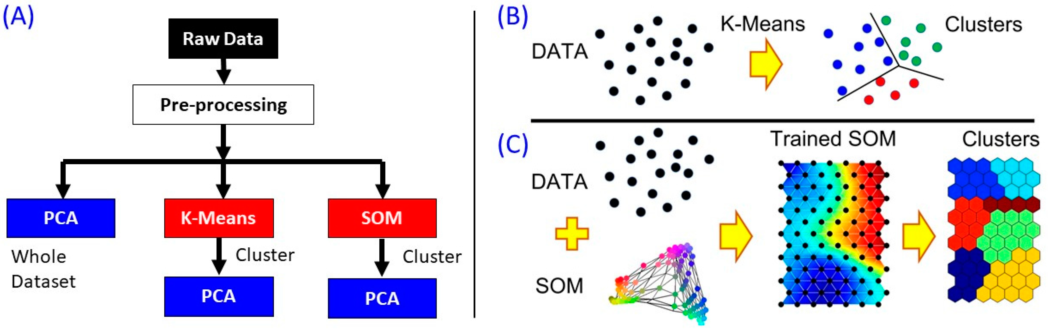
The raw datasets were preprocessed to extract only the key variables of unsupervised learning. An overview summary of the key variables and their definitions is shown in Table 1. The dataset was also checked for any emissions levels exceeding set limits by US-EPA [1] and it was found that all samples were below the emission limits for light-duty vehicles and light-duty trucks.

2.3. Data Analysis

The dataset of vehicles with model year 2022 was first used to show the detailed analysis tools and discussions of results derived from unsupervised machine learning analytics (Figure 1). This particular vehicle model year was also the source of the most peculiar trends in clusters of emission results, as shown in the results and discussion sections. Then, the datasets of other model years, 2015 to 2023, were added to conduct a more comprehensive analysis of the peculiar trends observed in the 2022 dataset. In general, the number of observations in each working dataset for the various vehicle model years was as follows: 4390 for 2015; 4116 for 2016; 4077 for 2017; 4164 for 2018; 4061 for 2019; 3815 for 2020; 3549 for 2021; 3580 for 2022; and 2850 for 2023. In total, there were 34,602 observations from nine vehicle model years. The number of observations in any model year was well above the suggested minimum number of samples for clustering analysis [20].

2.3.1. K-Means Implementation

The K-Means algorithm for clustering was implemented via the SAS-JMP software that uses the FASTCLUS procedure [21]. The optimal number of clusters was determined via the fit statistic Cubic Clustering Criterion (CCC), which has larger values at better fit models. The range of 2 to 10 clusters were tested iteratively and the optimal number of K-Means clusters was indicated by the maximum CCC.

2.3.2. SOM Implementation

The SOM algorithm available via the MATLAB R2013a add-in SOM Toolbox [17] was used instead of the SOM in SAS-JMP, as the former is more amenable to model configuration by user compared to the latter. A rectangular topographic map of hexagonal lattice of size 15 neurons by 12 neurons constituted the SOM model. This map size meets the size requirement for SOM to have enough datapoints that can hit most of the map neurons (best matching units, or BMU). The rectangular map was chosen over the cylindrical and toroid maps that were also available from the Toolbox due to its lower quantization error during preliminary testing of the SOM models. The other details of the rectangular SOM and its coded implementation in MATLAB can be checked in the supplementary materials in the online repository for this work [19]. The optimal number of clusters from the trained SOM was determined using the Davies–Bouldin Index (DBI), which must have a minimum value at optimal cluster size [17]. The range of 2 to 10 clusters were tested iteratively and the optimal number of rectangular SOM clusters was indicated by the minimum DBI.

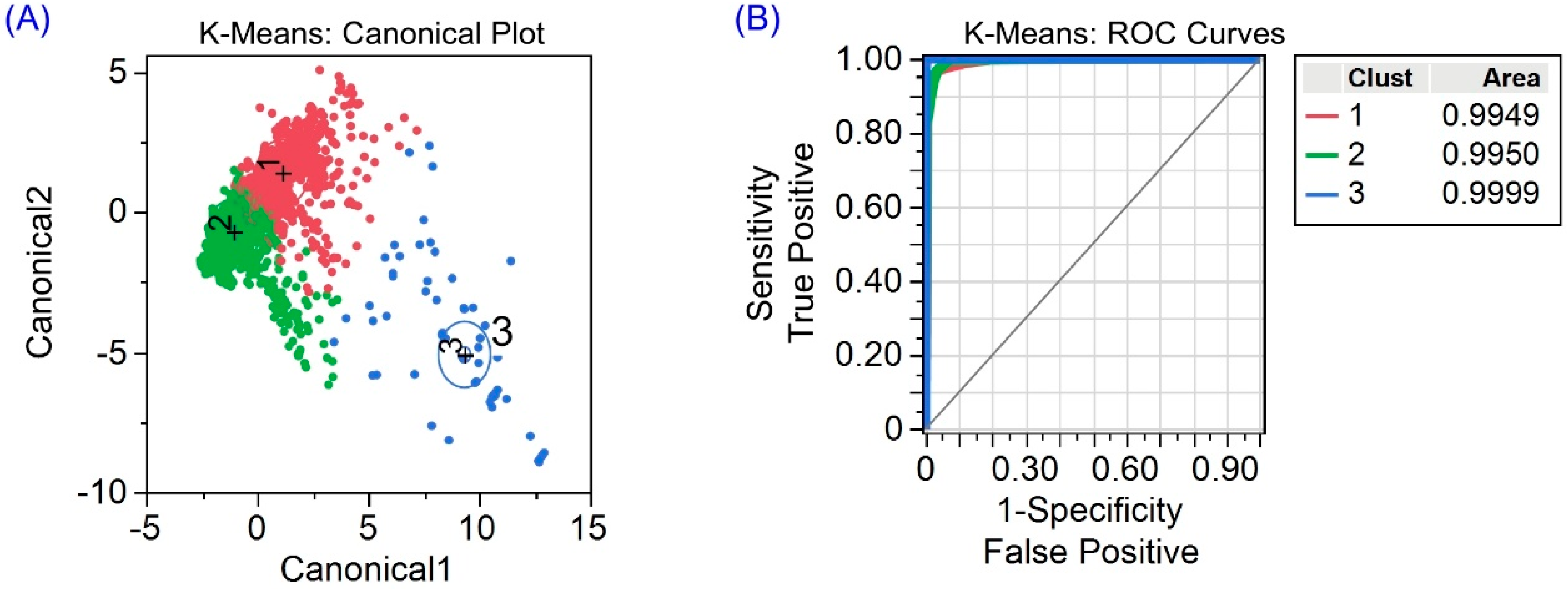
2.3.3. Linear Discriminant Analysis

To evaluate the performance of the clusters from K-Means and SOM as separating planes of the dataset, linear discriminant analysis (LDA) in SAS-JMP [14] was done on all the working variables against the cluster assignments. This analysis was the only supervised learning step in the data analysis. Canonical plots were created to visually show the clusters in terms of the canonical variables. The prediction rates of the clusters were also determined. The receiver operating characteristic (ROC) curve of each cluster on the training data was also calculated to determine the trade-off between the sensitivity and (1-specificity) across a series of cut-off points through the clusters.

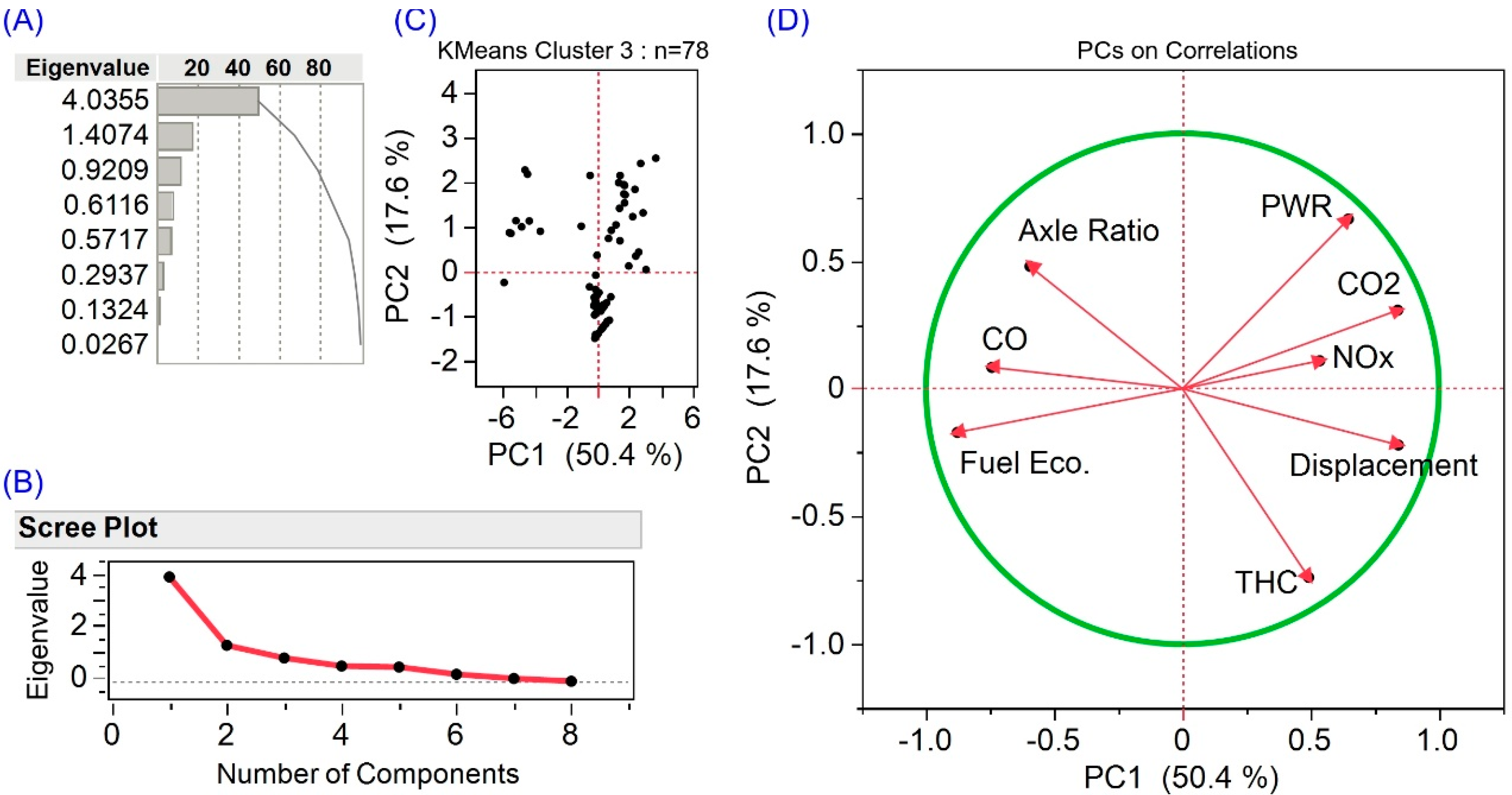
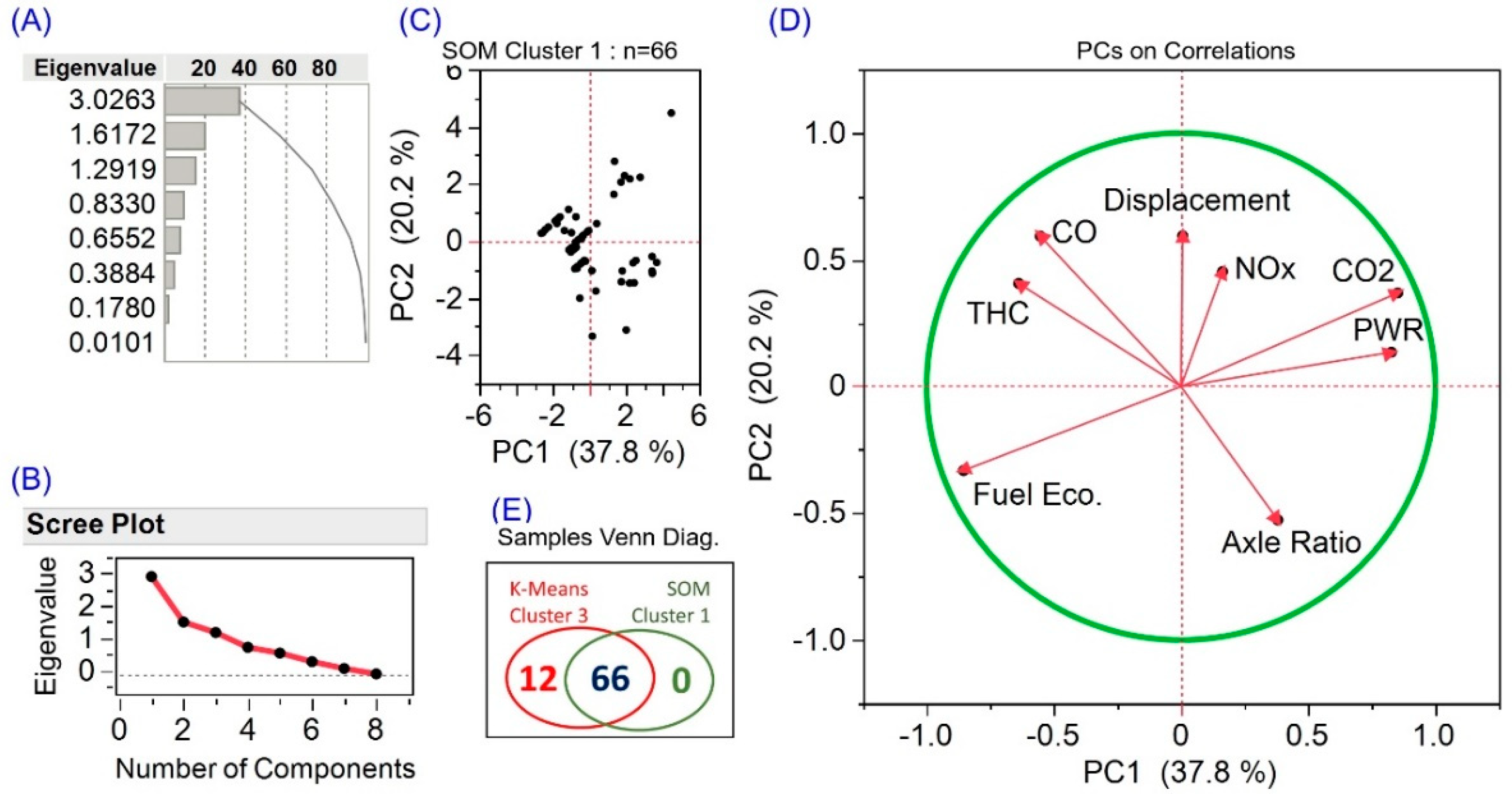
2.3.4. PCA Implementation

PCA was implemented via the SAS-JMP software [14]. The eigenvalues of the principal components (PCs) were evaluated to determine the data variance captured by the first two PCs (PC1 and PC2), which were then used as projection axes on two-dimensional loadings plots to render the trends of all the variables relative to each other.

3. Results and Discussion

Data re-projection onto the first few principal components (PCs) was done to reduce the dimensionality of the multivariate dataset, hence simplifying the comparison of variable trends. With this technique, variable trends in the whole (unsegmented) dataset were compared with the segmented dataset resulting from K-Means and SOM clustering. Then, statistical testing of model fits on the whole dataset and pertinent clusters was done to test the significance of parameter statistics.

3.1. Whole Dataset Fuel Economy and Emissions

When looking at the whole dataset projected onto the first few PCs (Figure 2), it was found that the first two PCs were enough to capture most of the variabilities in the dataset. That is, the eigenvalues of the first two PCs were higher compared to the residual eigenvalues after the first two PCs (Figure 2A,B). The combined PC1 and PC2 projections can explain 60.8% of the data variability. The score plot of the samples when projected on PC1 and PC2 (Figure 2C) shows some samples are far from the centroid, which indicates the possibility of a unique outliers cluster [10]. These outliers increase the variance of the data, which must be reduced to minimize uncertainties in statistic parameters [14]. Variance reduction can be done through data segmentation such as K-Means and SOM clustering. The loadings plot (Figure 2D) shows the direction (from the center (0, 0)) of variables relative to each other. For example, Fuel Economy is opposite the direction of all emissions variables THC, CO, CO_2, and NO_x, which means there is an inverse relationship of Fuel Economy with the emissions variables. As the variables approach orthogonal relation, for example THC with either PWR or Axle Ratio, the correlation becomes negligible. Displacement and CO₂ emission almost coincide, which indicates direct proportionality.

3.2. Clustered Dataset Fuel Economy and Emissions

The implementation and testing of clustering algorithms in segmenting the dataset into groups of similar attributes was done using K-Means and SOM. The optimal number of clusters was determined, then the clusters with distinct trends were examined further to elucidate variable trends.

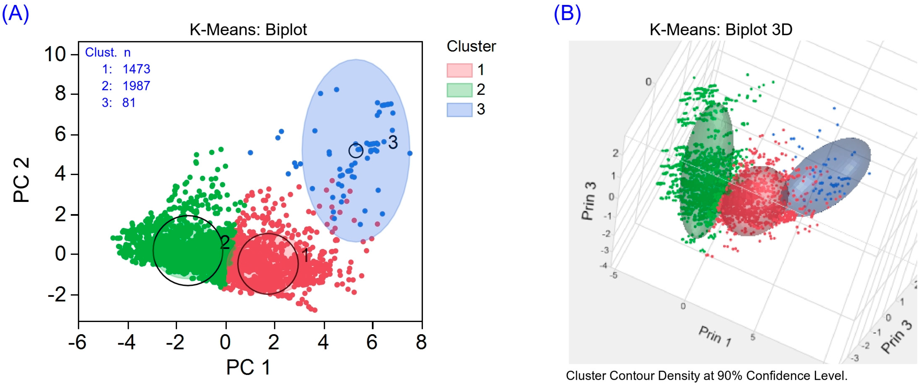
3.2.1. K-Means Clustering

The results of K-Means clustering are shown in Figure 3 and Figure 4. The optimal number of clusters, which was found to be three, resulted in distinct segmentation of the whole dataset. A visual representation of the segmentation is evident in Figure 3, which shows the projection of the cluster-coded samples onto the first two PCs (Figure 3A) and onto the first three PCs (Figure 3B). The results of LDA on these three clusters (Figure 4) confirmed that the three clusters achieve a very high area under the ROC (AUC), which is in the range 0.9949–0.9999. AUC is the probability that a classifier will rank a randomly chosen positive instance higher than a randomly chosen negative one, with AUC = 1.0 being a perfect classifier and AUC = 0.5 being a uniformly random classifier [14]. Hence, the three clusters from the K-Means clustering meet the requirements for a set of good segmentation planes for the dataset. The classification scores of these three clusters are summarized in

Table 2. Linear discriminant analysis prediction scores and rates for the K-Means clusters. LDVs model year is 2022.

Actual	Predicted Count			Predicted Rate
Cluster	1	2	3	1	2	3
1	1270	87	0	0.936	0.064	0.000
2	26	2115	2	0.012	0.986	0.001
3	2	0	76	0.038	0.000	0.962
Total Count: 3580	Percent Misclassified: 3.32%			Entropy R-square: 0.848

. The prediction rates of the three clusters are close to one, with an overall percent misclassification of only 3.22%. The trends within each of these clusters were then examined using PCA (Figure 5).

As an unsupervised learning technique, K-Means is not guaranteed to produce clusters containing equal numbers of samples. Clusters 1 and 2 were assigned 1357 and 2144 samples, respectively, whereas Cluster 3 was assigned 79 samples (out of the 3580 total samples). When applying PCA in each cluster, Clusters 1 and 2 demonstrated variable trends similar to the whole dataset (see supplementary material for these results), whereas Cluster 3 showed a peculiar trend (Figure 5). For Cluster 3, the CO levels were directly proportional to the Fuel Economy levels (Figure 5D), which had the opposite relation when considering the whole dataset (Figure 2D). The Axle Ratio was also directly proportional to the CO levels in K-Means Cluster 3, but it did not have any effect on CO levels on average in the whole dataset (Figure 2D). The same trend exists for Axle Ratio and THC, with Axle Ratio inversely proportional to the THC levels in K-Means Cluster 3, but not having any effect on THC levels on average in the whole dataset (Figure 2D).

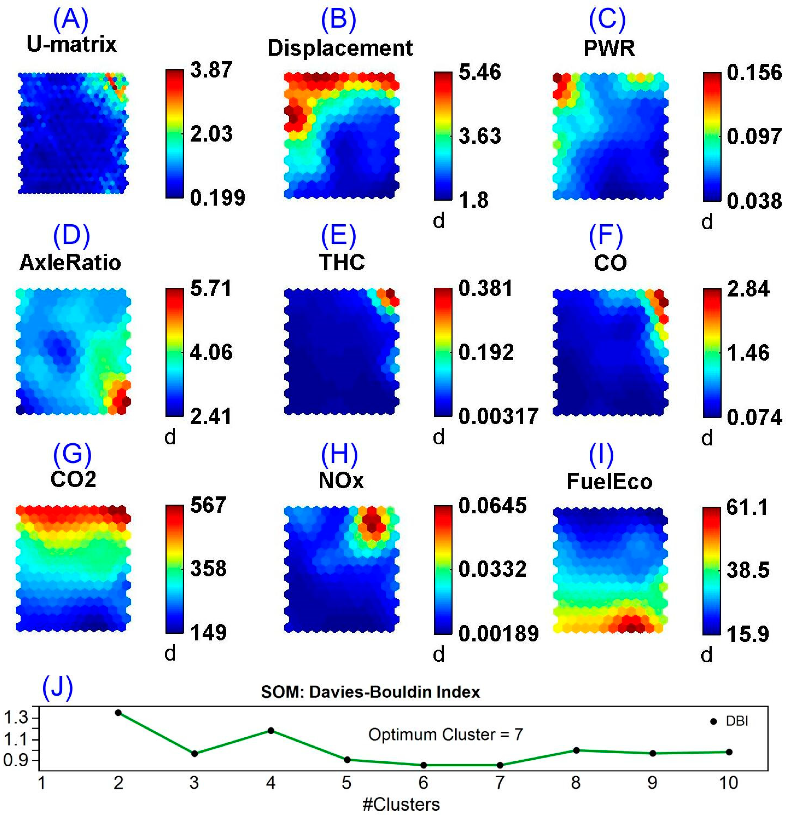
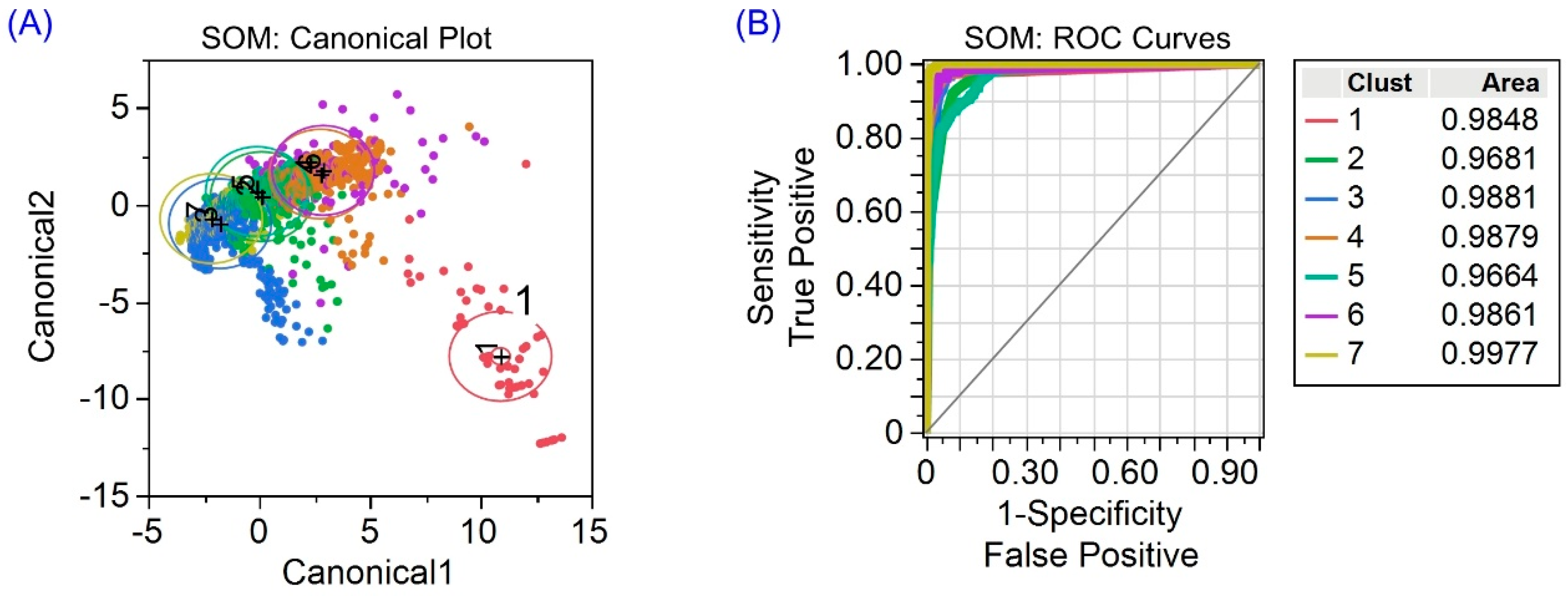
3.2.2. Self-Organizing Maps Clustering

The results of SOM clustering are shown in Figure 6 and Figure 7. A unique set of results from SOM are the projections of the variables onto component planes (Figure 6B,I) after the SOM model training on the dataset. These are visual renderings of the relative levels of the variables at a specific neuron position (a unit cell on the map) on the maps. The U-matrix, or unified distance matrix (Figure 6A), represents the Euclidean distance between the codebook vectors of neighboring neurons, and the high values in the map indicate regions of samples of distinct attribute levels [17]. The optimal number of clusters for the model year 2022 dataset was seven, which resulted in the minimum DBI during the SOM clustering (Figure 6J). Unlike the K-Means, which showed very distinct segmentation of the dataset on a 2D canonical plot, SOM produced a set of clusters that have some overlaps when projected onto the first two canonical variables in the LDA (Figure 7A). This is expected, as the number of SOM clusters is greater than the first few canonical variable representations. Nonetheless, the AUCs of the seven SOM clusters were in the range of 0.9664-0.9977 (Figure 7B), which are still high AUC values [10]. The classification scores of these seven SOM clusters, which are in the prediction rate range of 0.794–0.955 (

Table 3. Linear discriminant analysis prediction scores and rates for the SOM clusters. LDVs model year is 2022.

Actual	Predicted Count
Cluster	1	2	3	4	5	6	7
1	63	0	0	2	0	1	0
2	0	800	24	7	25	7	15
3	0	93	913	0	105	1	0
4	0	45	0	476	47	0	4
5	0	71	7	0	399	0	1
6	0	8	0	17	1	100	0
7	0	3	30	0	13	0	304
Actual	Predicted Rate
Cluster	1	2	3	4	5	6	7
1	0.955	0.000	0.000	0.030	0.000	0.015	0.000
2	0.000	0.911	0.027	0.008	0.028	0.008	0.017
3	0.000	0.084	0.821	0.000	0.094	0.001	0.000
4	0.000	0.079	0.000	0.832	0.082	0.000	0.007
5	0.000	0.149	0.015	0.000	0.834	0.000	0.002
6	0.000	0.063	0.000	0.135	0.008	0.794	0.000
7	0.000	0.009	0.086	0.000	0.037	0.000	0.869
Total Count: 3580		Percent Misclassified: 14.72%			Entropy R-Square: 0.753

), are not as high as those of K-Means and have an overall percent misclassification of 14.72%.

The segmentation of samples in each SOM cluster was examined for any commonality with the K-Means clusters. The samples captured by SOM Cluster 1 are subset samples of the K-Means Cluster 3. That is, of the 78 samples in K-Means Cluster 3, 66 were also assigned to the SOM Cluster 1 (Figure 8E). This indicates that these two clusters covered almost the same segment of the dataset. This can be visually verified in Figure 4A and Figure 7A, showing these clusters as extreme groups in the first two canonical variables in LDA. The prediction rate of the SOM Cluster 1 is at 0.955, which is the second highest rate in the eight clusters (Table 3).

3.3. Performance of K-Means and SOM Clustering

The data segmentation results of the K-Means and the SOM algorithms are not exactly the same, but they both capture clusters of samples, K-Means Cluster 3 and SOM Cluster 1, that exhibit similar trends. These clusters show some variable trends that the whole dataset does not represent. These findings demonstrate the capability of K-Means and SOM in extracting hidden trends in the bigger dataset. Of the 3580 total working samples, 78 (or 2.18 % of 3580) are assigned to K-Means Cluster 3, and 66 (or 1.84% of 3580) are assigned to SOM Cluster 1. This is the kind of data mining problem where clustering algorithms K-Means and SOM are needed—detecting outliers that are of smaller percentages of the data, but that can have attributes with correlations different from the whole dataset [10,11]. The LDA results (Figure 4 and Figure 7; Table 2 and Table 3) also confirm this consistency of clustering results for K-Means Cluster 3 and SOM Cluster 1. Between the two clustering techniques, however, K-Means has a lower cluster misclassification rate of 3.32% (Table 2) than that of SOM at 14.72% (Table 3).

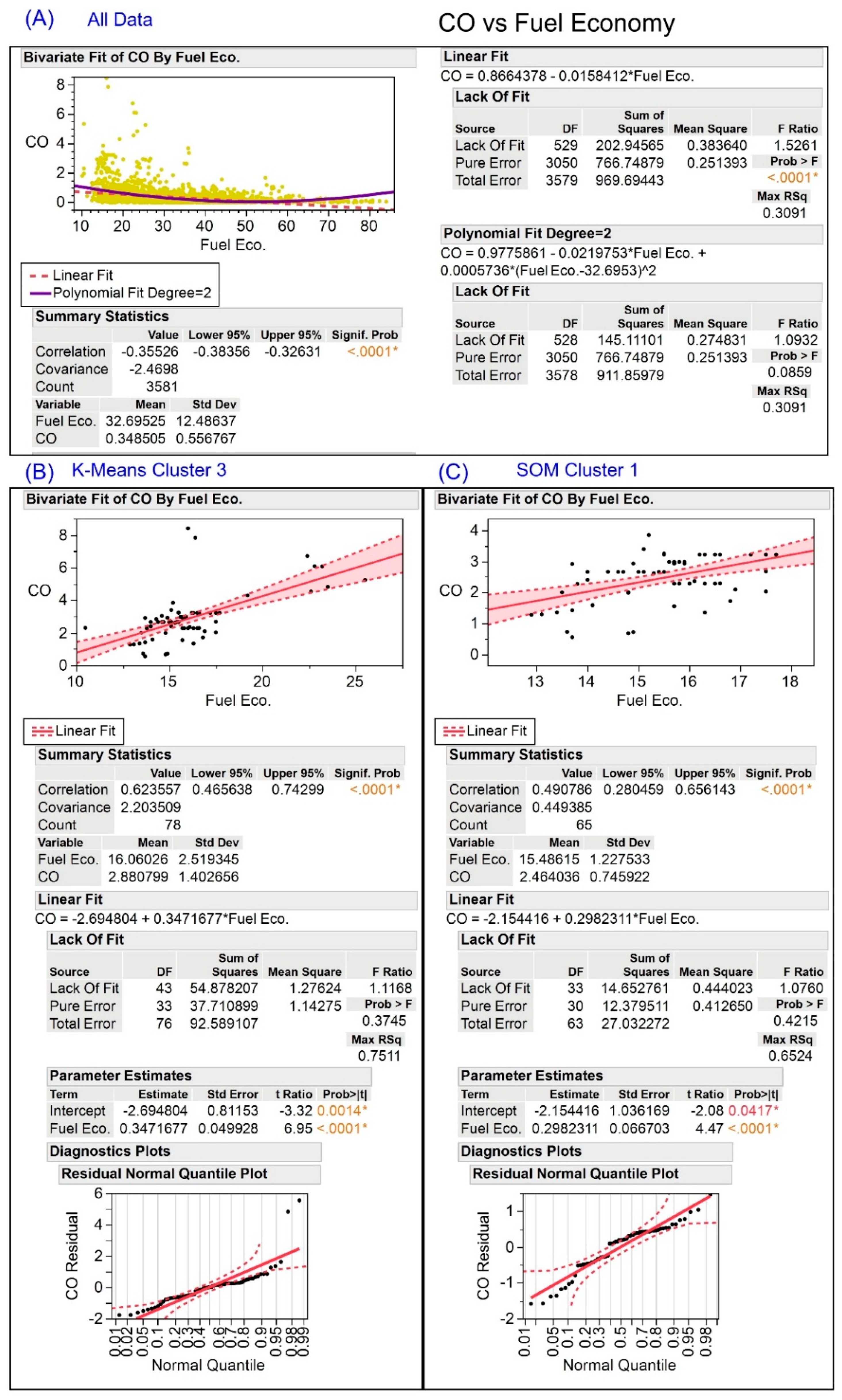
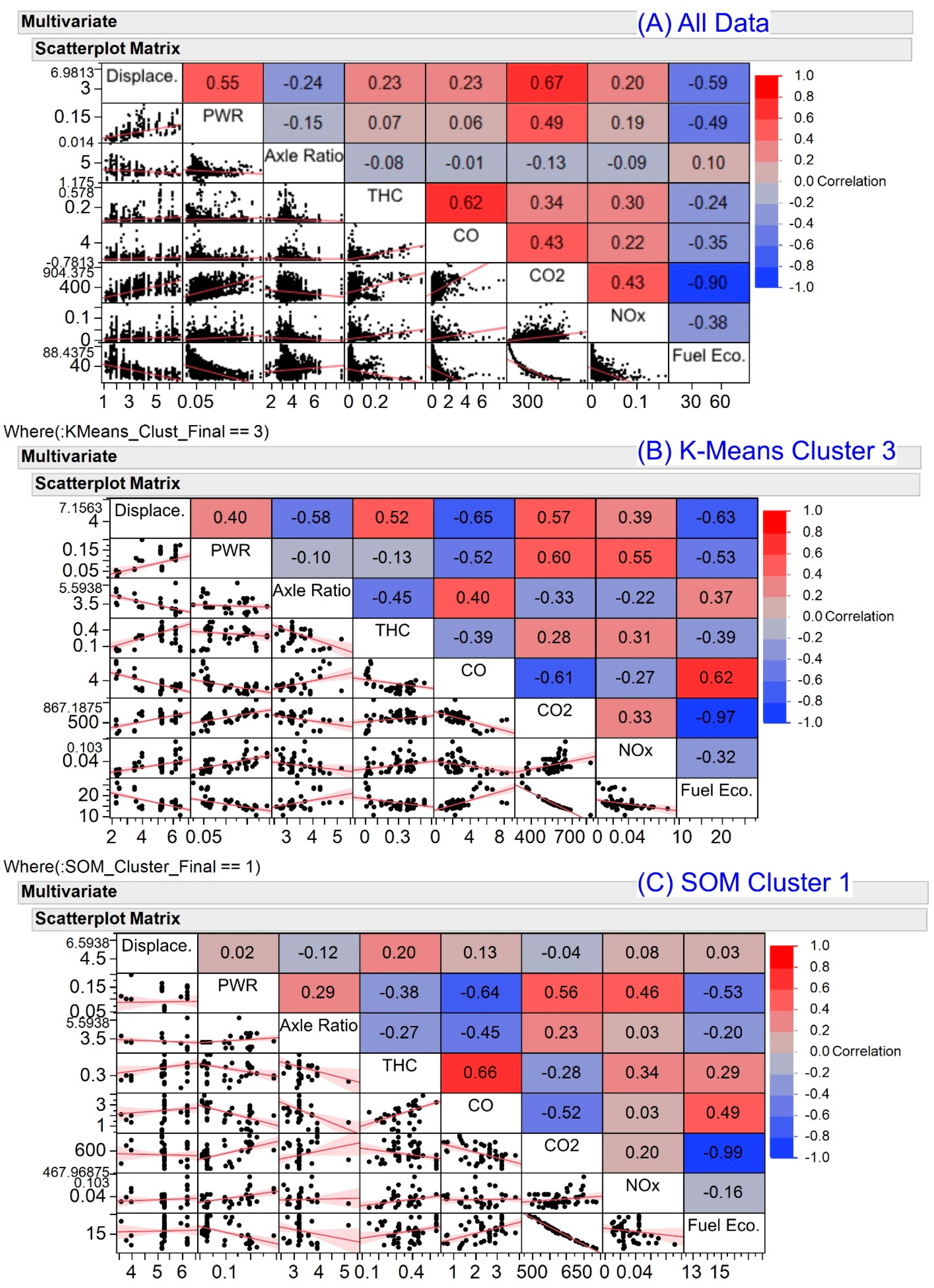
3.4. Bivariate Analysis on CO vs. Fuel Economy

Among the various clusters determined, Cluster 3 from K-Means and Cluster 1 from SOM showed peculiar trends regarding the relation of CO emissions to Fuel Economy. A bivariate analysis of this relation was done to determine summary statistics and model fitting. Figure 9 shows a summary of the results for the whole dataset samples (Figure 9A), K-Means Cluster 3 samples (Figure 9B), and SOM Cluster 1 samples (Figure 9B). These results show that the correlation of CO emissions and Fuel Economy is statistically different between the calculation on the whole dataset and the calculation on the clusters. The direction of proportionality changes from negative correlation r = (−) 0.355 (Figure 9A) on the whole dataset to a positive correlation on the clusters; r = (+) 0.62 on K-Means Cluster 3 (Figure 9B) and r = (+) 0.491 on SOM Cluster 1 (Figure 9C). Model fitting on the data was also done to test the null hypothesis that the slopes of proportionality are zero, which would mean no functional linear relation between CO and Fuel Economy. Rejecting this null hypothesis would mean the slopes are statistically different from zero, which eliminates the possibility of random errors causing the correlations. The calculated slopes of the linear models fitted to the clusters data are different from zero; they are 0.347 CO (g/mi)/MPG and 0.298 CO (g/mi)/MPG for K-Means Cluster 3 and SOM Cluster 1, respectively, with [Prob>|t|] less than 0.001 at a 5% significance level (Figure 9B,C). In addition, the lack-of-fit test was done to confirm the fitting performance of the models; it tested whether the lack-of-fit error is zero (equivalently means significantly smaller than pure error) [14]. With F-statistic probabilities [Prob>F] = 0.0.2349 and 0.4215 for K-Means Cluster 3 and SOM Cluster 1, respectively, the lack-of-fit test cannot reject the null hypothesis at a 5% significance level, which means that the lack-of-fit error is statistically zero. This confirms the inference that the linear models for CO vs. Fuel Economy statistically fit the data in each cluster. These results mean that when looking at the whole dataset, the statistical inference is that the CO emission decreases with Fuel Economy. On the other hand, when looking at the two clusters, K-Means Cluster 3 and SOM Cluster 1, the statistical inference is that CO emission is increasing with increasing Fuel Economy.

3.5. Other Notable Variable Correlations

There are other notable trends seen on the whole dataset and on the K-Means Cluster 3 and SOM Cluster 1 as shown by the multivariate correlation graphs in Figure 10. Power-to-weight (PWR) and Fuel Economy correlation values are close to each other, with negative values r = (−) 0.49, r = (−) 0.53, and r = (−) 0.53 for the whole dataset, K-Means Cluster 3, and SOM Cluster 1, respectively. This means an increasing PWR results in decreasing Fuel Economy whether considering the whole dataset or the clusters. On the other hand, the PWR shows a change in direction of correlation with CO when analyzed from the whole dataset compared to the clustered dataset. PWR and CO have almost negligible correlation if analyzed in the whole dataset, with r = (+) 0.06, but they have a negative correlation, seen in values r = (−) 0.52 and r = (−) 0.64, in K-Means Cluster 3 and SOM Cluster 1, respectively.

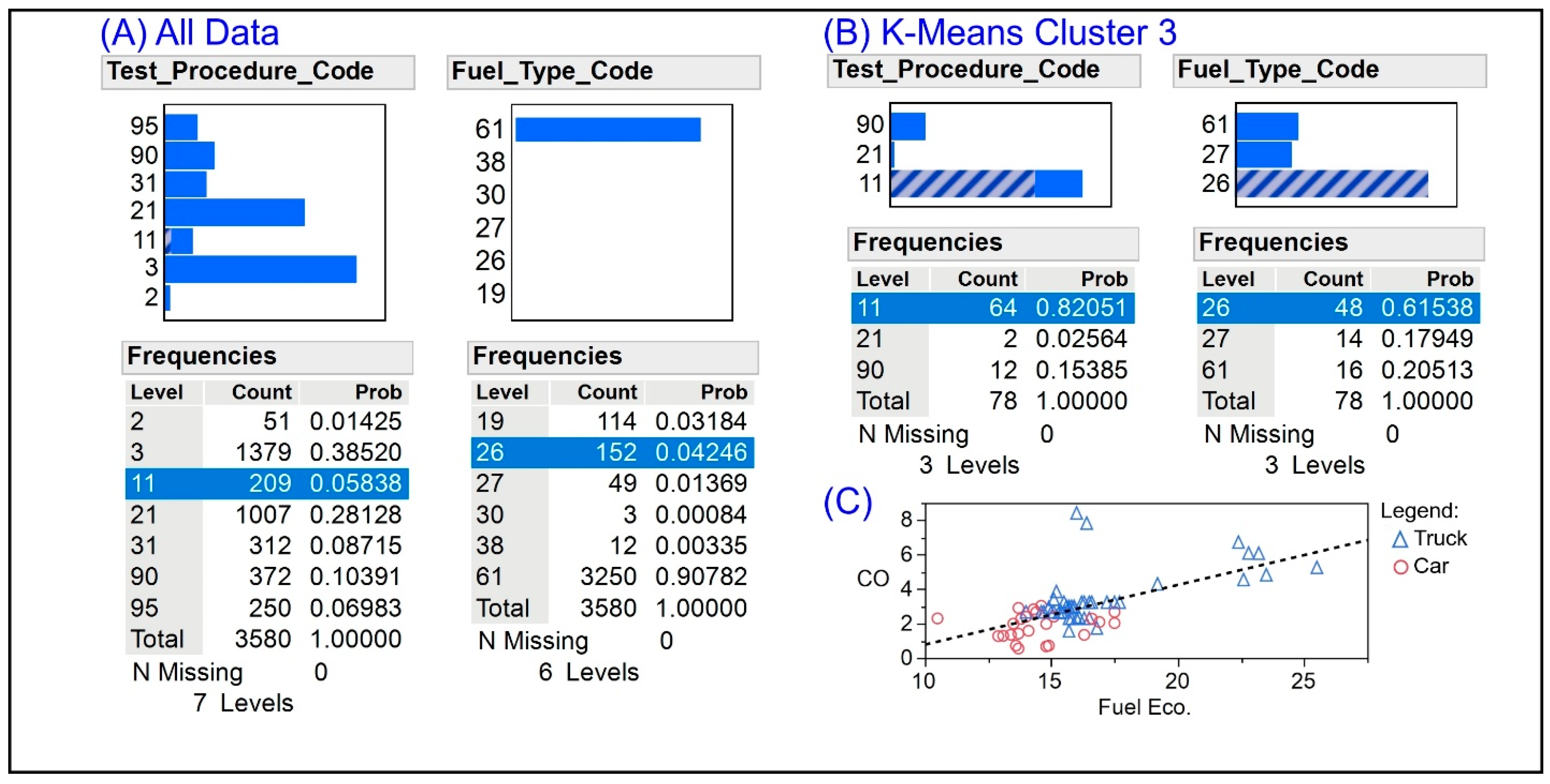
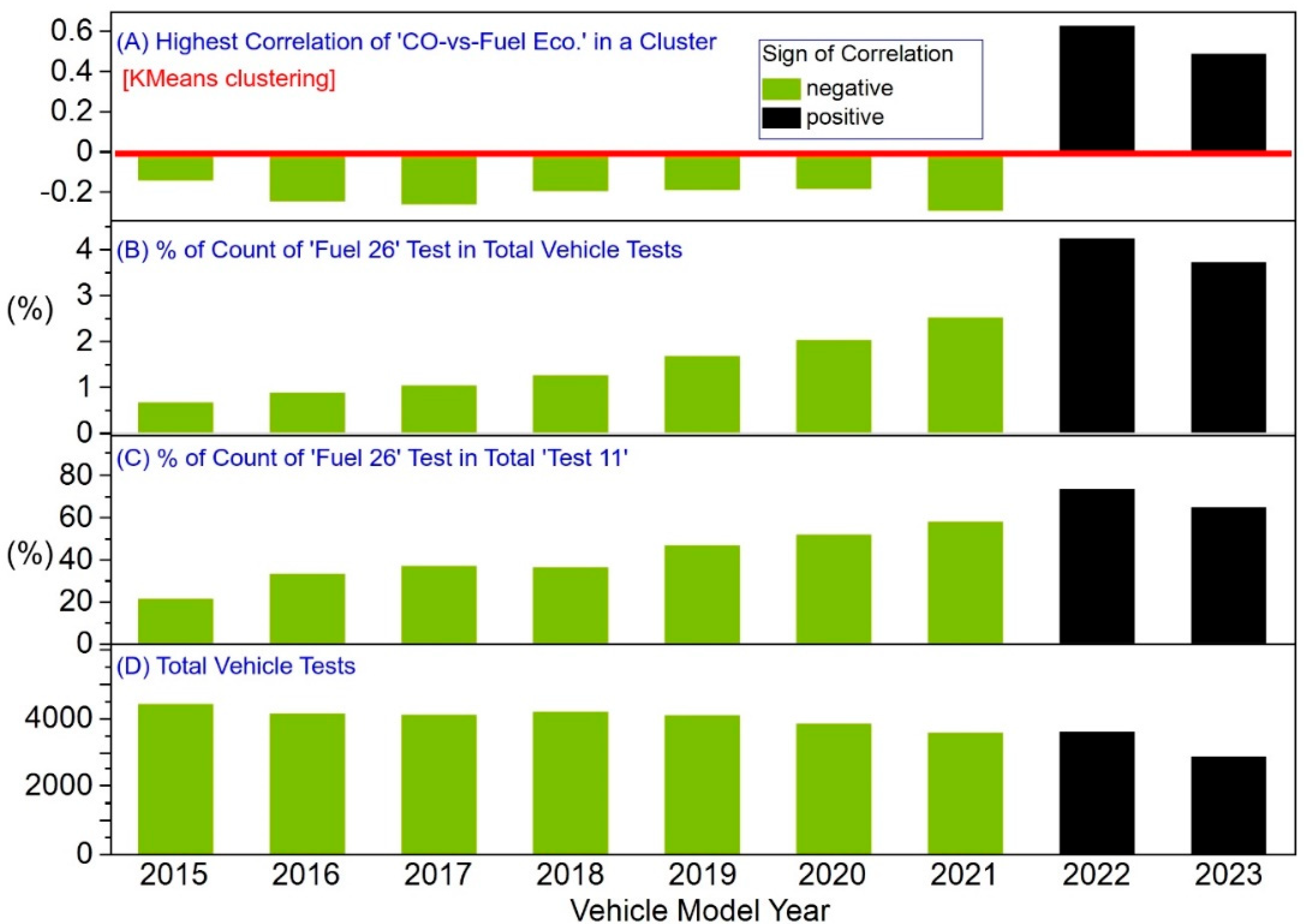
3.6. Unsupervised Learning Uncovers an Impending Anomaly

With the clusters K-Means Cluster 3 and SOM Cluster 1 for LDVs model year 2022 showing peculiar trends relative to the whole dataset, the distributions of clustered data based on the categorical variables in the dataset were evaluated. These categorical variables were not used in the unsupervised clustering of the dataset done in the preceding discussions, but their dominance in the K-Means Cluster 3 and SOM Cluster 1 could help explain the peculiar CO-vs.-Fuel Economy correlations. Two categorical variables were found to have dominant levels in K-Means Cluster 3 and SOM Cluster 1: Test Procedure and Fuel Type. Figure 11 shows a distribution analysis of Test Procedure and Fuel Type in the whole 2022 dataset and in K-Means Cluster 3. Note that because SOM Cluster 1 is a subset of K-Means Cluster 3, and because K-Means has a lower misclassification rate (3.32% in Table 2) than SOM, the distribution analysis used only the clustered K-Means Cluster 3 against the whole dataset. The categorical level codes for the Test Procedure and Fuel Type are based on the US-EPA coding described in

Table 4. US-EPA testing procedure codes and descriptions [16].

Test Procedure Code	Test Procedure Description
2	CVS 75 and later (w/o canister load); Constant Volume Sampler (CVS)-75 is an emission certification driving mode for gasoline, LPG, and older diesel vehicles
3	HWFE, which is the Highway Fuel Economy Driving Schedule, represents highway driving conditions under 60 mph
11	Cold CO, which is the cold temperature testing procedures for measuring CO
21	Federal Test Procedure (FTP) fuel 2-day exhaust (w/canister load)
31	Federal Test Procedure (FTP) fuel 3-day exhaust
90	US06, which is a high acceleration aggressive driving schedule that is often identified as the “Supplemental FTP” driving schedule
95	SC03, which is the Air Conditioning “Supplemental FTP” driving schedule

and

Table 5. US-EPA testing fuel type codes and descriptions [16].

Fuel Type Code	Fuel Type Description
19	Federal Cert Diesel 7–15 PPM Sulfur
26	Cold CO Regular (Tier 2)
27	Cold CO Premium (Tier 2)
30	Cold CO Diesel 7–15 ppm Sulfur
38	E85 (85% Ethanol 15% EPA Unleaded Gasoline)
61	Tier 2 Cert Gasoline

.

To perform a more comprehensive evaluation of the influence of Test Procedure and Fuel Type, the datasets for other vehicle model years 2015, 2016, 2017, 2018, 2019, 2020, 2021, and 2023 were also analyzed in the same data analytics workflow applied to model year 2022 as depicted in Figure 1. This allowed for a trends analysis that leveraged on the strength of the K-Means algorithm to test the hypothesis that increasing the use of Test Procedure 11 and Fuel 26 results in a higher tendency to have positive correlation of CO vs. Fuel Economy. This concept is based on the fact that segmentation of dataset via K-Means results in more distinct clusters that exhibit particular trends as the number of observations increases [10,20]. That is, higher percentages of a particular test or fuel type implemented on LDVs should result in higher chances of their being clustered together due to the higher dominance of their influence on the features used in clustering. If the influence of a test procedure or a fuel type is not peculiar, then it should be clustered by K-Means with the majority of the dataset amid the increasing percentage of its count in the dataset; otherwise, its peculiar influence would stand out with its increasing count in the dataset. Figure 12 shows the graphical results of this analysis.

The use of Fuel 26 as part of US-EPA’s emissions testing standard fuel set has been increasing through the years (Figure 12B). The use of Fuel 26 in Test Procedure 11 has also been increasing through the years (Figure 12C). Applying the concept that the increasing sample size of a particular treatment can affect the clustering of samples with peculiar feature trends [20], it can be inferred that Fuel 26 and Test Procedure 11 may have been the factors behind the positive correlation of CO and Fuel Economy (Figure 12A). Isolating the effects of each factor may be difficult because Fuel 26 has been increasingly used in Test Procedure 11 in recent years. Also worth noting is that the originators of the data samples in the clusters with positive correlation of CO vs. Fuel Economy are the vehicle manufacturers (see captions of Figure 5 and Figure 8) and not a US-EPA testing center. This was found in both the LDVs model years 2022 and 2023. Considering that manufacturers follow established test procedures and use test fuel standards independent of each other and US-EPA, the independence of sampling was guaranteed in the clustered datasets. This also eliminates the possible issue of US-EPA testing centers being factors in the peculiar trends. This leads the inquiry to the chemistry of Fuel 26 being used in Test Procedure 11.

The exact causal relations of these two factors cannot be determined using the datasets in this work, as strong correlation is not sufficient to model any mechanistic relations of variables. However, the correlations can be used to warrant some actions by US-EPA, such as re-evaluating the chemistry of Fuel 26 when it is used in Test Procedure 11. Fuel 26 and test Procedure 11 supposedly simulate a cold start of a vehicle [16]. Previous works have investigated the case of cold-start emissions and compared the standard limits of California’s LDVs surveillance program and found that the cold-start emissions in the actual setup produced lower levels than the levels predicted by the standard model, and concluded that the importance of cold-start emissions may be overstated in emission inventories [22]. This also leads to the question of how accurate is using Fuel 26 with Test Procedure 11 in modeling actual driving conditions, and some of the literature [23] has already demonstrated some techniques in such an inquiry. Such evaluation may elucidate necessary adjustments to the established testing procedures and standard fuels [7,8].

3.7. CO vs. Fuel Economy Anomaly in the Big Picture of LDVs Market

The fuel economy of vehicles has been a common parameter used in the valuation of vehicle performance, not just in the US, but also worldwide [24,25]. Hence, vehicle manufacturers have been aiming to constantly improve fuel economy ratings. Part of having these vehicles be available for purchase by consumers, however, is the need for certifications issued by regulatory agencies such as US-EPA that consider emissions performance in addition to fuel economy ratings. Emissions performance has been the center of legislative and regulatory issues; for example, the state of California in the US has been imposing stricter emission standards relative to US-EPA standards [26,27]. A higher fuel economy rating does not necessarily mean a good emissions rating, as shown in this work (Figure 9). However, emissions ratings are the result not solely of vehicle engine design, but also of the implemented testing procedures and the test fuels used in testing, as shown in this work (Figure 11, Table 4 and Table 5). Therefore, it is necessary for regulatory agencies to make sure the test procedures and test fuels are appropriate, especially for LDVs that are averaging sales of around 70–90 million vehicles per year [2]. Amid the efforts for the massive use of electric vehicles, the use of petrol-based vehicles is still the largest fraction of transportation worldwide, especially the LDVs category [28]. Gasoline and diesel are still the major energy sources, but new technologies are diffusing into the LDV sector in response to fuel efficiency and emissions standards [29].

If emissions test procedures and test fuel types are found to be not the issue, then the findings in this work (Figure 9) imply that certain LDVs are emitting higher CO levels at higher Fuel Economies. The fact that the positive correlation of CO and Fuel Economy was detected in the test LDVs datasets that meet emissions limits alludes to the questions: “What is the trend of CO and Fuel Economy in the LDVs that did not meet emissions limits?” and “Are Test Procedure and Fuel Type still probable significant factors for any emissions anomaly in the LDVs that did not meet emissions limits?” These are questions that this work may not be able to answer due to dataset limitations. Nonetheless, the data analytics workflow demonstrated in this work (Figure 1) would still be appropriate in answering such questions.

4. Conclusions

This study demonstrated that unsupervised machine learning algorithms PCA, K-Means, and SOM can elucidate trends in a large collection of testing datasets on vehicle fuel economy and emissions of LDVs collected by US-EPA. The combined application of these techniques shows that variable trends for the whole dataset can be different from the variable trends within certain K-Means and SOM clusters. Among the bivariate trends that significantly change, the trends between the Fuel Economy and CO emission levels are evidently significantly different when calculated on the whole dataset and when calculated in clusters. CO vs. Fuel Economy has a negative correlation in the whole dataset, but it has positive correlations in certain sample clusters. Upon performing a comprehensive analysis of datasets for LDVs model years 2015 to 2023, it was found that Test Procedure and Fuel Type could be the significant factors behind the positive correlation of CO and Fuel Economy. Specifically, the increasing use of Test Fuel 26 used in Test Procedure 11 was found to be the probable cause. This is an impending anomaly, as the use of Fuel 26 in emissions testing with Test Procedure 11 of US-EPA has been increasing through the years. With the finding that the clustered data samples with positive CO-vs.-Fuel Economy correlation all came from vehicle manufacturers that independently conduct the standard testing procedures, it is suggested that the chemistry of using Fuel 26 in performing Test Procedure 11 be re-evaluated by US-EPA.

References

1. US-EPA. Light-Duty Vehicles and Light-Duty Trucks: Clean Fuel Fleet Exhaust Emission Standards; US-EPA: Washington, DC, USA, 2016; Volume EPA-420-B-16-006. [Google Scholar]
2. IEA. World Energy Investment; International Energy Agency (IEA): Paris, France, 2020. [Google Scholar]
3. Hui, H.; Jin, L. A Historical Review of the U.S. In Vehicle Emission Compliance Program and Emission Recall Case; The International Council on Clean Transportation (ICCT): Washington, DC, USA, 2017. [Google Scholar]
4. US-EPA. Emission Standards Reference Guide: All EPA Emission Standards. Available online: https://www.epa.gov/emission-standards-reference-guide/all-epa-emission-standards (accessed on 9 April 2022).
5. US-EPA. Revised 2023 and Later Model Year LightDuty Vehicle GHG Emissions Standards: Regulatory Impact Analysis; US-EPA Assessment and Standards Division Office of Transportation and Air Quality: Washington, DC, USA, 2021. [Google Scholar]
6. US-EPA. 2014–2017 Progress Report: Vehicle and Engine Compliance Activities; US-EPA: Washington, DC, USA, 2019; Volume 420R19003, p. 122. [Google Scholar]
7. UNECE. Sustainable Development Brief No. 4: Emissions Testing for Cars and Environmental Regulations; United Nations Economic Commission for Europe (UNECE): Geneva, Switzerland, 2016. [Google Scholar]
8. US-EPA. Revisions to Test Methods, Performance Specifications, and Testing Regulations for Air Emission Sources; EPA, Ed.; Environmental Protection Agency (EPA): Washington, DC, USA, 2016; Volume EPA-HQ-OAR-2014-0292. [Google Scholar]
9. Trunk, G.V. A Problem of Dimensionality: A Simple Example. IEEE Trans. Pattern Anal. Mach. Intell. 1979, PAMI-1, 306–307. [Google Scholar] [CrossRef] [PubMed]
10. Gareth James, D.W.; Trevor, H.; Robert, T. An Introduction to Statistical Learning, 1st ed.; Springer: New York, NY, USA, 2013. [Google Scholar]
11. Hastie, T.; Tibshirani, R.; Friedman, J. The Elements of Statistical Learning: Data Mining, Inference, and Prediction, 2nd ed.; Springer: Berlin/Heidelberg, Germany, 2009. [Google Scholar]
12. Kanungo, T.; Mount, D.M.; Netanyahu, N.S.; Piatko, C.D.; Silverman, R.; Wu, A.Y. An efficient k-means clustering algorithm: Analysis and implementation. IEEE Trans. Pattern Anal. Mach. Intell. 2002, 24, 881–892. [Google Scholar] [CrossRef]
13. Jolliffe, I.T.; Cadima, J. Principal component analysis: A review and recent developments. Philos. Trans. R. Soc. A Math. Phys. Eng. Sci. 2016, 374, 20150202. [Google Scholar] [CrossRef] [PubMed] [Green Version]
14. SAS. JMP® 16 Documentation Library; SAS Institute Inc.: Cary, NC, USA, 2022. [Google Scholar]
15. Fortela, D.L.B.; Crawford, M.; DeLattre, A.; Kowalski, S.; Lissard, M.; Fremin, A.; Sharp, W.; Revellame, E.; Hernandez, R.; Zappi, M. Using Self-Organizing Maps to Elucidate Patterns among Variables in Simulated Syngas Combustion. Clean Technol. 2020, 2, 156–169. [Google Scholar] [CrossRef]
16. US-EPA. Data on Cars used for Testing Fuel Economy. Available online: https://www.epa.gov/compliance-and-fuel-economy-data/data-cars-used-testing-fuel-economy (accessed on 9 April 2022).
17. Kohonen, T. MATLAB Implementations and Applications of the Self-Organizing Map; Unigrafia Bookstore: Helsinki, Finland, 2014. [Google Scholar]
18. MathWorks MATrix LABoratory (MATLAB) R2013a; MathWorks: Natick, MA, USA, 2013.
19. Fortela, D.L. GitHub Repo: Unsupervised Learning to Elucidate Trends in Testing Data on Fuel Economy and Emissions of Light-Weight Vehicles. 2022. Available online: https://github.com/dhanfort/Cars22-FEandEmissions.git (accessed on 9 April 2022).
20. Henry, D.; Dymnicki, A.B.; Mohatt, N.; Allen, J.; Kelly, J.G. Clustering Methods with Qualitative Data: A Mixed-Methods Approach for Prevention Research with Small Samples. Prev. Sci. Off. J. Soc. Prev. Res. 2015, 16, 1007–1016. [Google Scholar] [CrossRef] [PubMed] [Green Version]
21. SAS. SAS/STAT 15.2 User’s Guide: The FASTCLUS Procedure; SAS, Ed.; SAS: Singapore, 2020. [Google Scholar]
22. Singer, B.C.; Kirchstetter, T.W.; Harley, R.A.; Kendall, G.R.; Hesson, J.M. A Fuel-Based Approach to Estimating Motor Vehicle Cold-Start Emissions. J. Air Waste Manag. Assoc. 1999, 49, 125–135. [Google Scholar] [CrossRef] [PubMed] [Green Version]
23. Khan, T.; Frey, H.C. Comparison of real-world and certification emission rates for light duty gasoline vehicles. Sci. Total Environ. 2018, 622–623, 790–800. [Google Scholar] [CrossRef] [PubMed]
24. Bansal, P.; Dua, R.; Krueger, R.; Graham, D.J. Fuel economy valuation and preferences of Indian two-wheeler buyers. J. Clean. Prod. 2021, 294, 126328. [Google Scholar] [CrossRef]
25. Sheldon, T.L.; Dua, R. How responsive is Saudi new vehicle fleet fuel economy to fuel-and vehicle-price policy levers? Energy Econ. 2021, 97, 105026. [Google Scholar] [CrossRef]
26. CARB. States That Have Adopted California’s Vehicle Standards under Section 177 of the Federal Clean Air Act; California Air Resources Board (CARB): Sacramento, CA, USA, 2021. [Google Scholar]
27. U.S. Congress. Clean Air Act. In United States Code Title 42 Chapter 85; U.S. Congress: Washington, DC, USA, 1990. [Google Scholar]
28. Briceno-Garmendia, C.; Qiao, W.; Foste, V. The Economics of Electric Vehicles for Passenger Transportation. In Mobility and Transport Connectivity Series, November 2022 ed.; The World Bank: Washington, DC, USA, 2022. [Google Scholar]
29. Frey, H.C. Trends in onroad transportation energy and emissions. J. Air Waste Manag. Assoc. 2018, 68, 514–563. [Google Scholar] [CrossRef] [PubMed]
Figure 1. Schematic of the data analysis workflow implemented in this study: (A) PCA, K-Means and SOM unsupervised learning techniques were applied; (B) cluster calculation by K-Means algorithm and (C) cluster calculation by SOM algorithm.
Cleantechnol 05 00021 g001
Figure 2. PCA results for the whole dataset. (A) Eigenvalues and their proportions, (B) scree plot of eigenvalues, (C) score plots of the samples on the PC1 and PC2, and (D) loadings plot of the variables on PC1 and PC2. LDVs model year is 2022.
Cleantechnol 05 00021 g002
Figure 3. Optimal clusters identified through K-Means clustering. (A) Clusters projected on the first two PCs-PC1 and PC2, and (B) clusters projected on the first three PCs-PC1, PC2, and PC3. LDVs model year is 2022.
Cleantechnol 05 00021 g003
Figure 4. Linear discriminant analysis canonical plot (A) and ROC curves (B) for the K-Means clusters. LDVs model year is 2022.
Cleantechnol 05 00021 g004
Figure 5. PCA trends in K-Means Cluster 3. (A) Eigenvalues and their proportions, (B) scree plot of eigenvalues, (C) score plots of the samples on the PC1 and PC2, and (D) loadings plot of the variables on PC1 and PC2. Note that the originators of the data samples clustered in K-Means Cluster 3 are the vehicle manufacturers that independently conduct the fuel economy and emissions tests. LDVs model year is 2022.
Cleantechnol 05 00021 g005
Figure 6. Performance of SOM in training on the input dataset. The optimal cluster number based on the Davies–Bouldin index (minimum) is seven clusters. The rendered maps are the denormalized values of variables (denoted by “d”) in their original units. LDVs model year is 2022.
Cleantechnol 05 00021 g006
Figure 7. Linear discriminant analysis canonical plot (A) and ROC curves (B) for the SOM clusters. LDVs model year is 2022.
Cleantechnol 05 00021 g007
Figure 8. PCA trends in SOM Cluster 1. (A) Eigenvalues and their proportions, (B) scree plot of eigenvalues, (C) score plots of the samples on the PC1 and PC2, and (D) loadings plot of the variables on PC1 and PC2. Note that the originators of the data samples clustered in SOM Cluster 1 are the vehicle manufacturers that independently conduct the fuel economy and emissions tests. LDVs model year is 2022.
Cleantechnol 05 00021 g008
Figure 9. Bivariate analysis and modeling between Fuel Economy and CO emissions in the (A) whole dataset, (B) K-Means Cluster 3 linear model fit with dashed lines as 95% confidence boundaries, and (C) SOM Cluster 1 linear model fit with dashed lines as 95% confidence boundaries. LDVs model year is 2022.
Cleantechnol 05 00021 g009
Figure 10. Multivariate correlation of variables on the (A) whole dataset, (B) K-Means Cluster 3, and (C) SOM Cluster 1. LDVs model year is 2022.
Cleantechnol 05 00021 g010
Figure 11. Distribution of data in the whole dataset (A) and the K-Means Cluster 3 (B) according to the Test Procedure and the Fuel Type used during testing. The level codes for the procedure and the fuel are based on the US-EPA codes. LDVs model year is 2022. The diagonal hashes on the bars in (A,B) visually indicate the features levels associated with the selection of the Fuel Type level 26 in the K-Means Cluster 3 (B). Subplot (C) is a bivariate plot of CO and Fuel Economy with datapoint legend for trucks and cars to show the locations of the K-Means Cluster 3 data relative to the linear model fit.
Cleantechnol 05 00021 g011
Figure 12. The potential effects of Fuel Type and Test Procedure, specifically “Fuel 26” and “Test 11” in the US-EPA emissions test standards, on the positive correlation of CO vs. Fuel Economy. (A) The highest correlation value of CO vs. Fuel Economy in a cluster after applying K-Means clustering; (B) percentage of number of tests that used Fuel 26 in the whole dataset from a vehicle model year; (C) percentage of number of tests that used Fuel 26 in the Test Procedure 11; (D) the total number of LDV tests in the dataset for a model year.
Cleantechnol 05 00021 g012