
Spatial Optimization of Conservation Practices for Sediment Load Reduction in Ungauged Agricultural Watersheds

Abstract
:1. Introduction
2. Materials and Methods
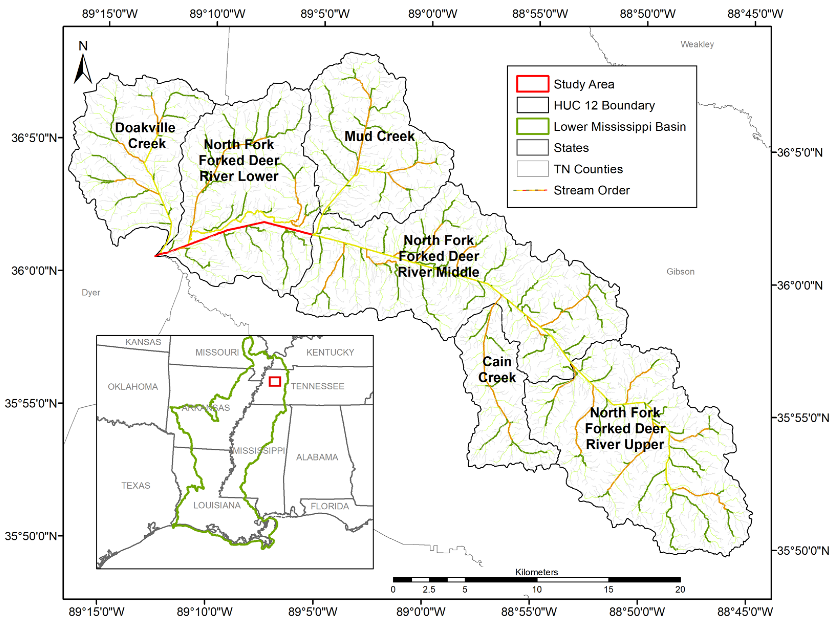
2.1. Study Area
2.2. The AnnAGNPS Model
2.3. Characterization and Modeling of Riparian Buffers
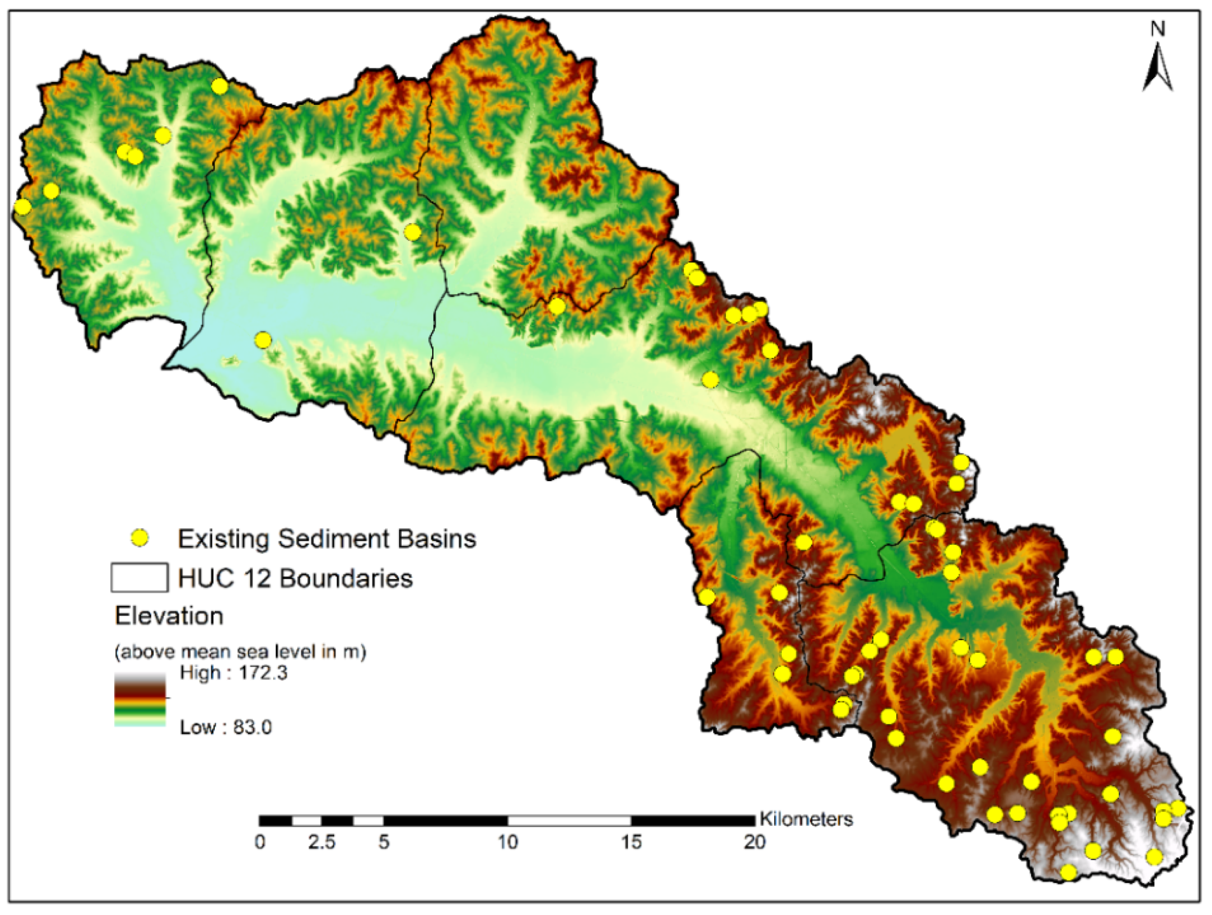
2.4. Characterization and Modeling of Constructed Sediment Basins
2.5. Baseline Conditions
2.5.1. Topography
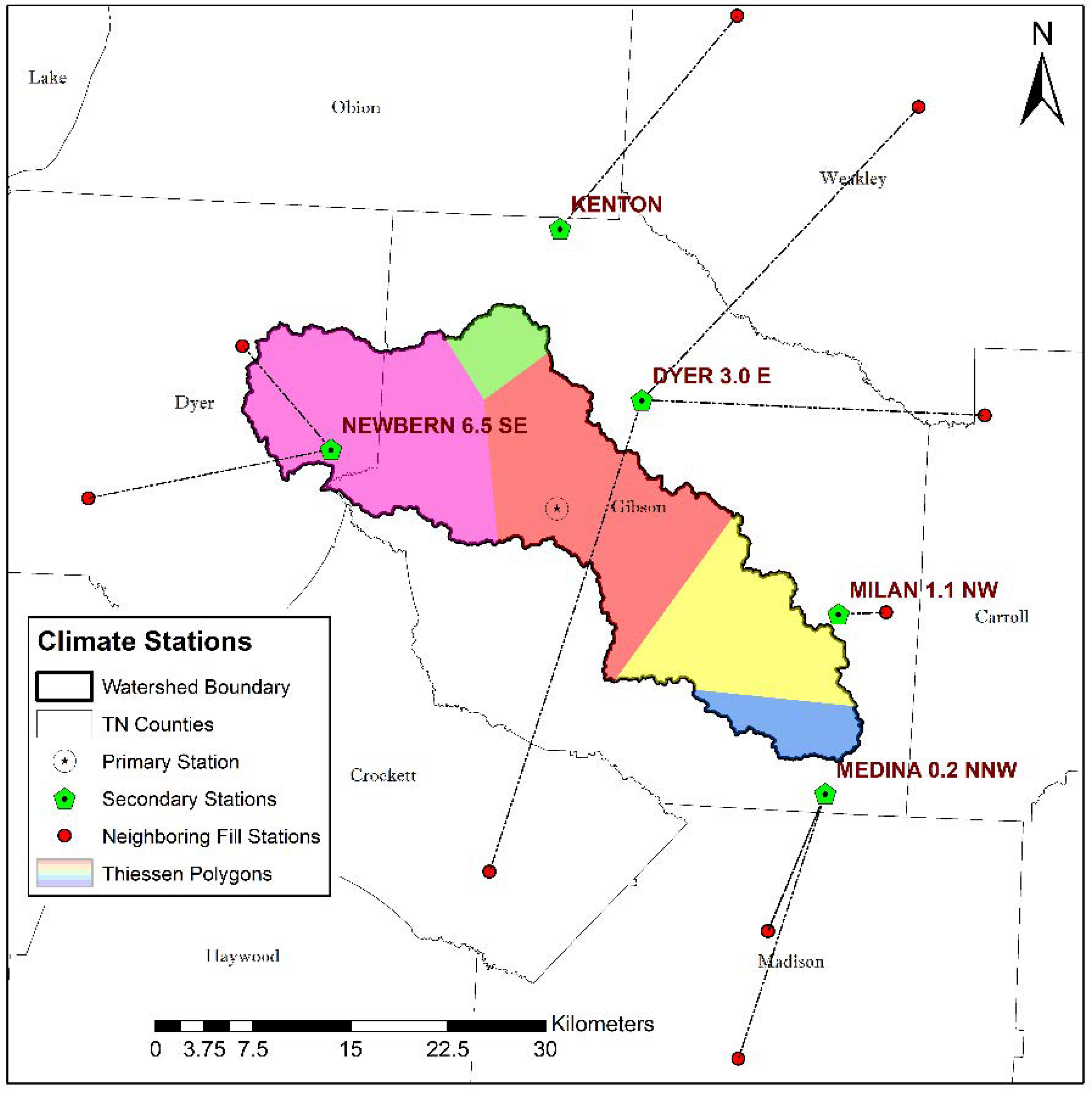
2.5.2. Climate
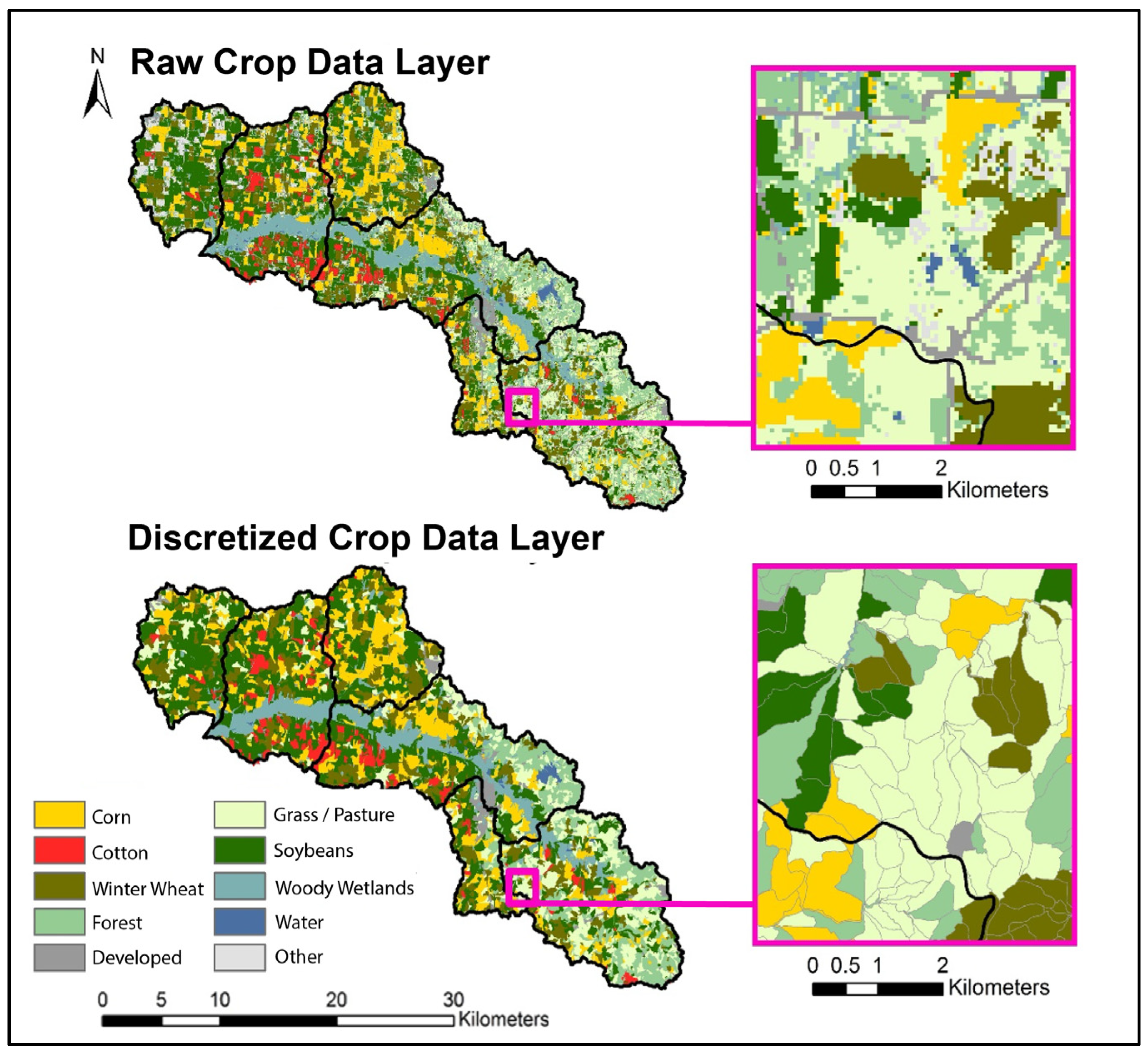
2.5.3. Soil
2.5.4. Management
2.6. Conservative Practices Scenarios
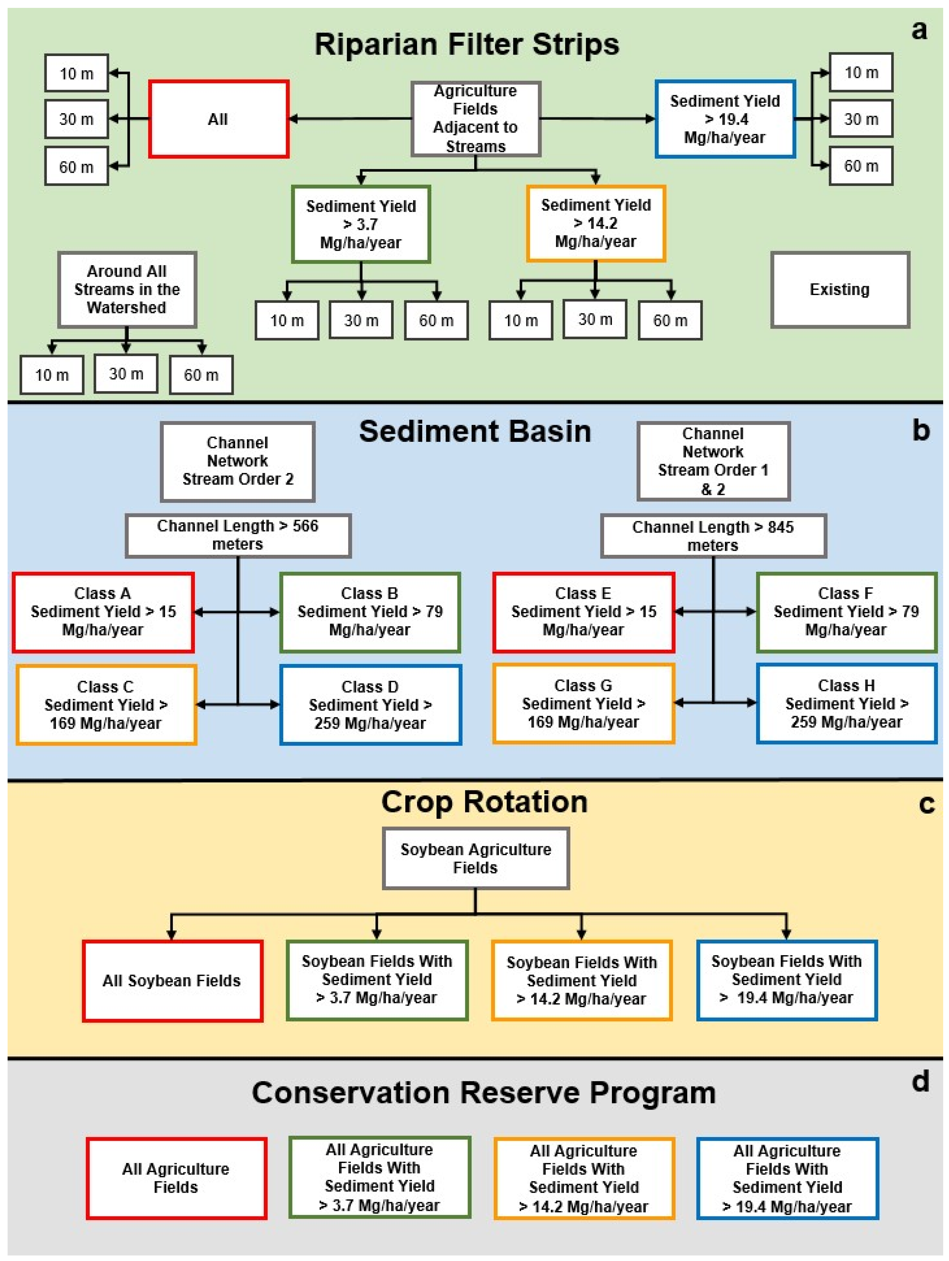
2.6.1. Riparian Buffer
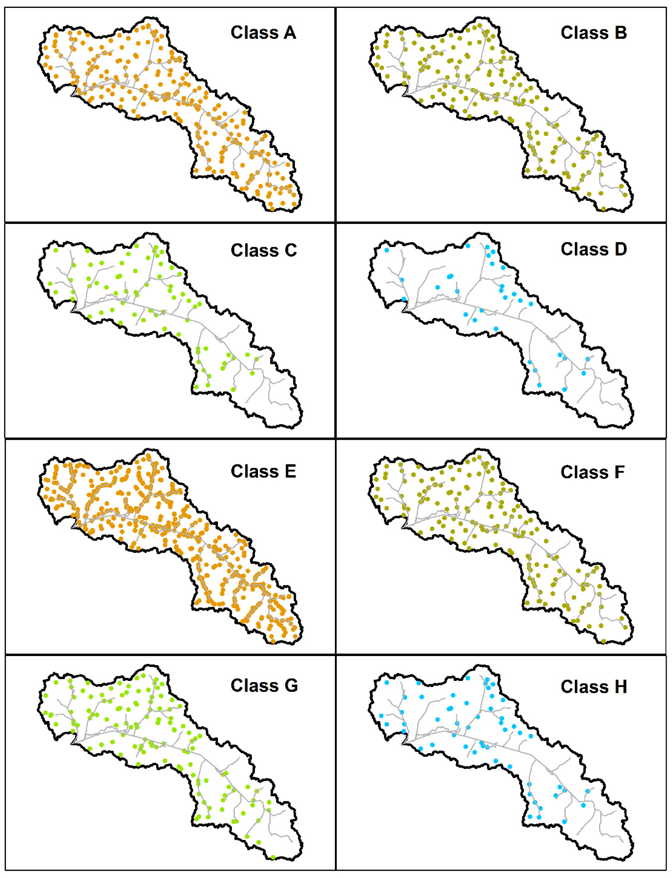
2.6.2. Sediment Basin
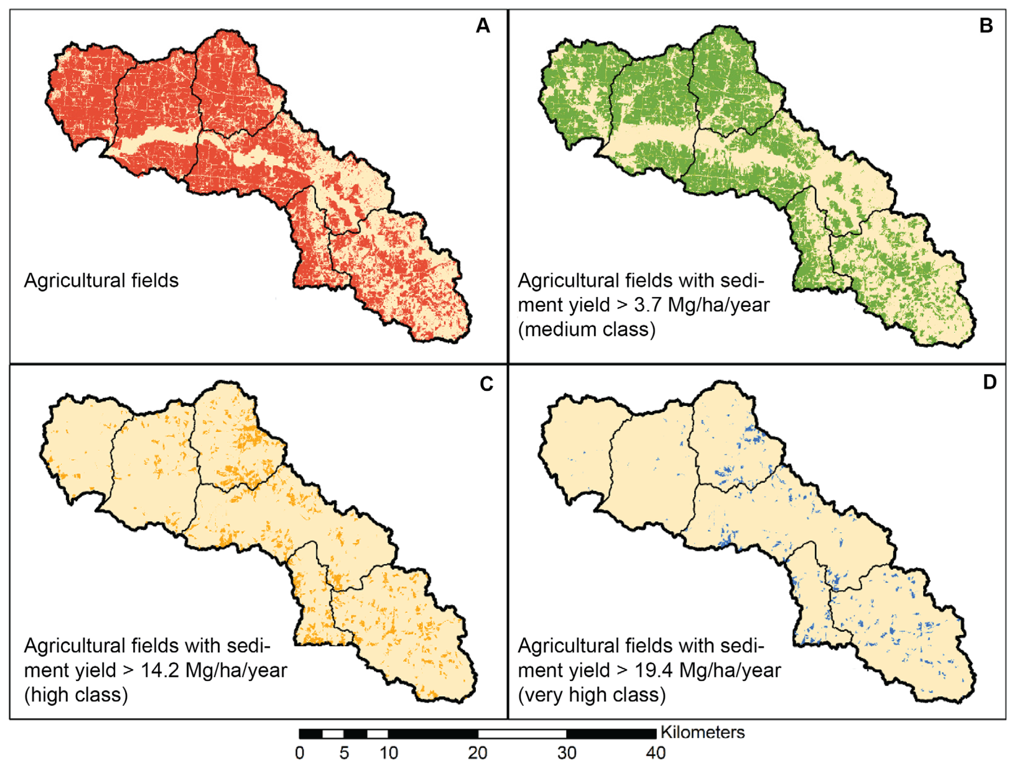
2.6.3. Crop Rotation
2.6.4. Conservation Reserve Program
2.6.5. Optimization and Comparison of Conservation Practice Scenarios
3. Results
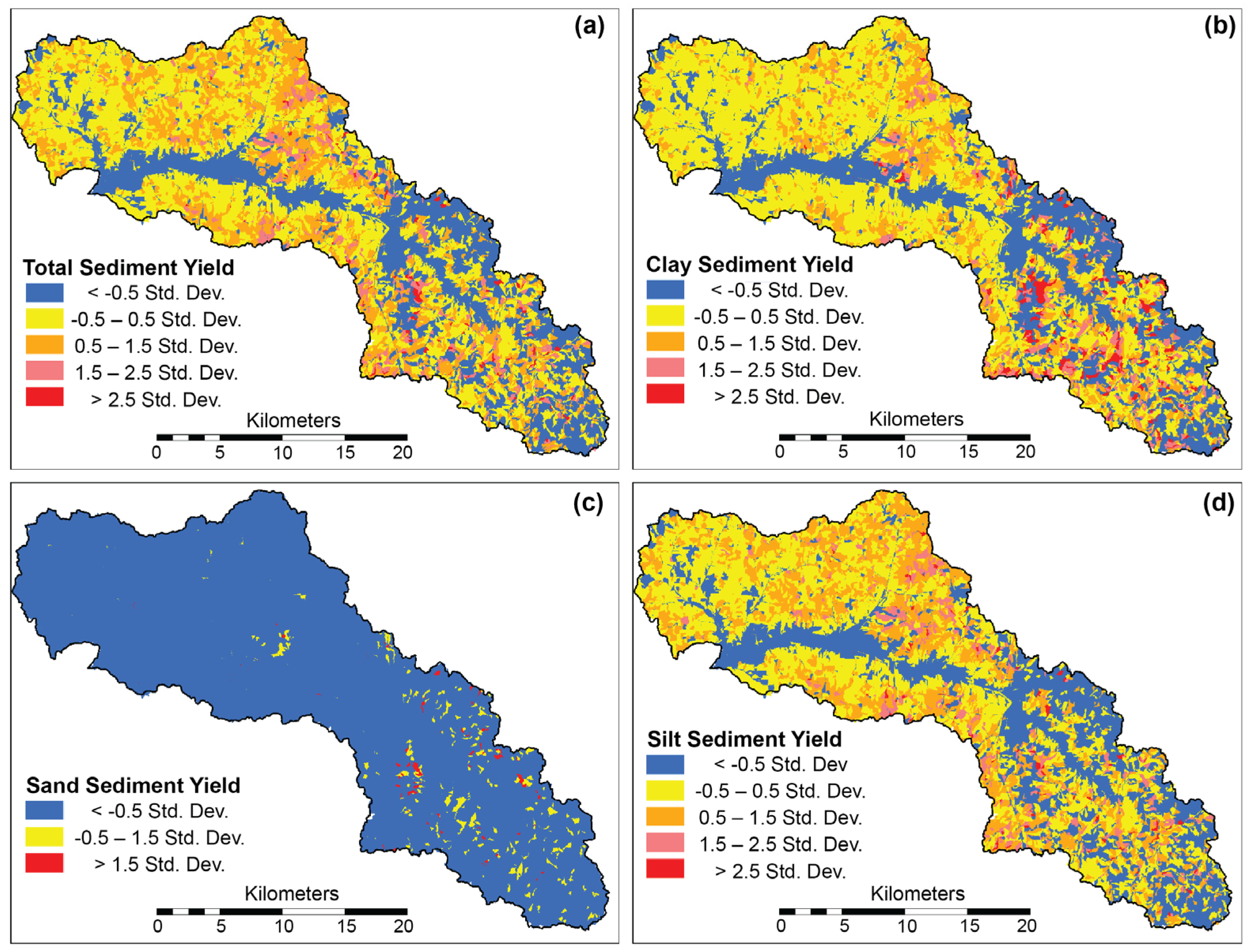
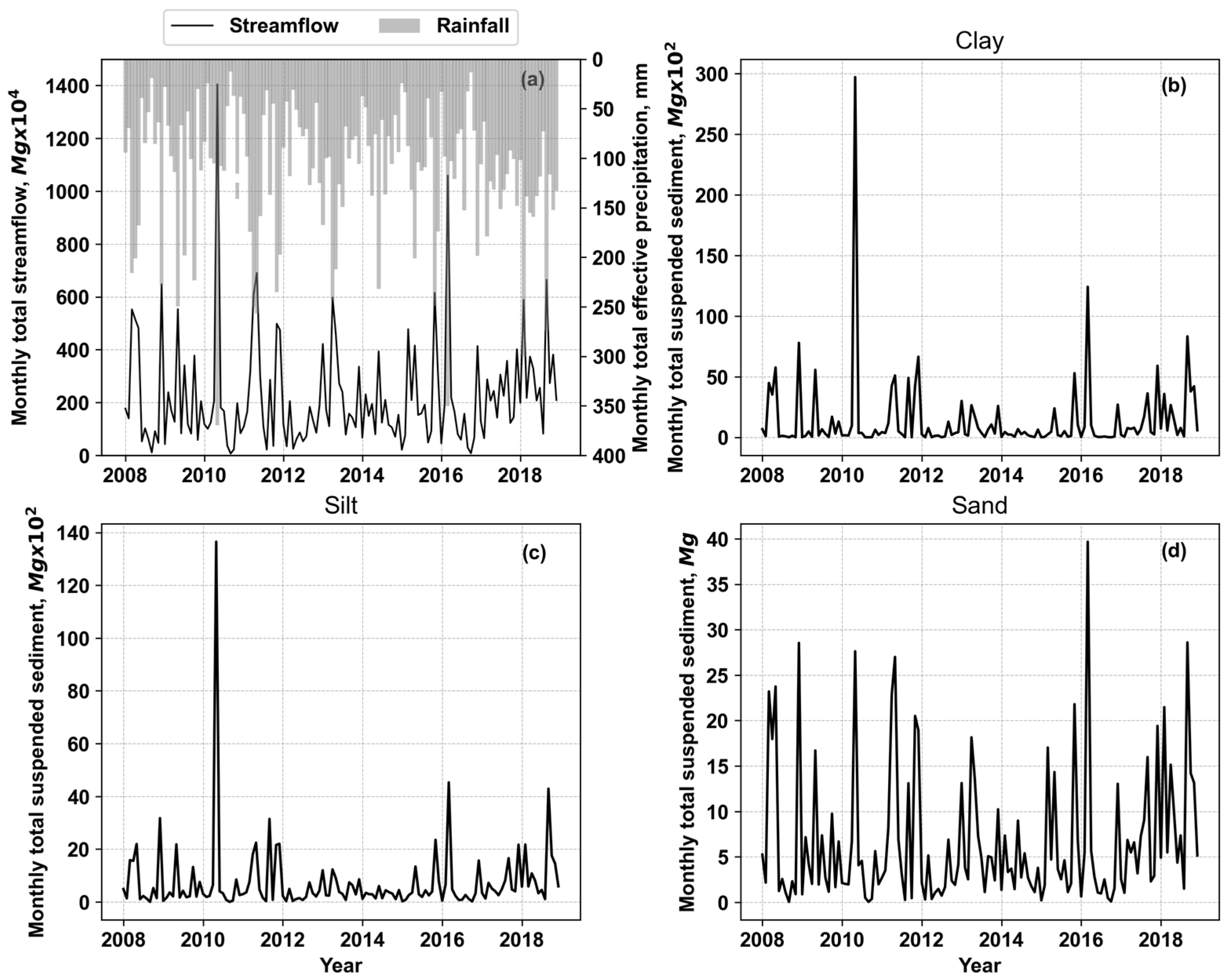
3.1. Baseline Conditions
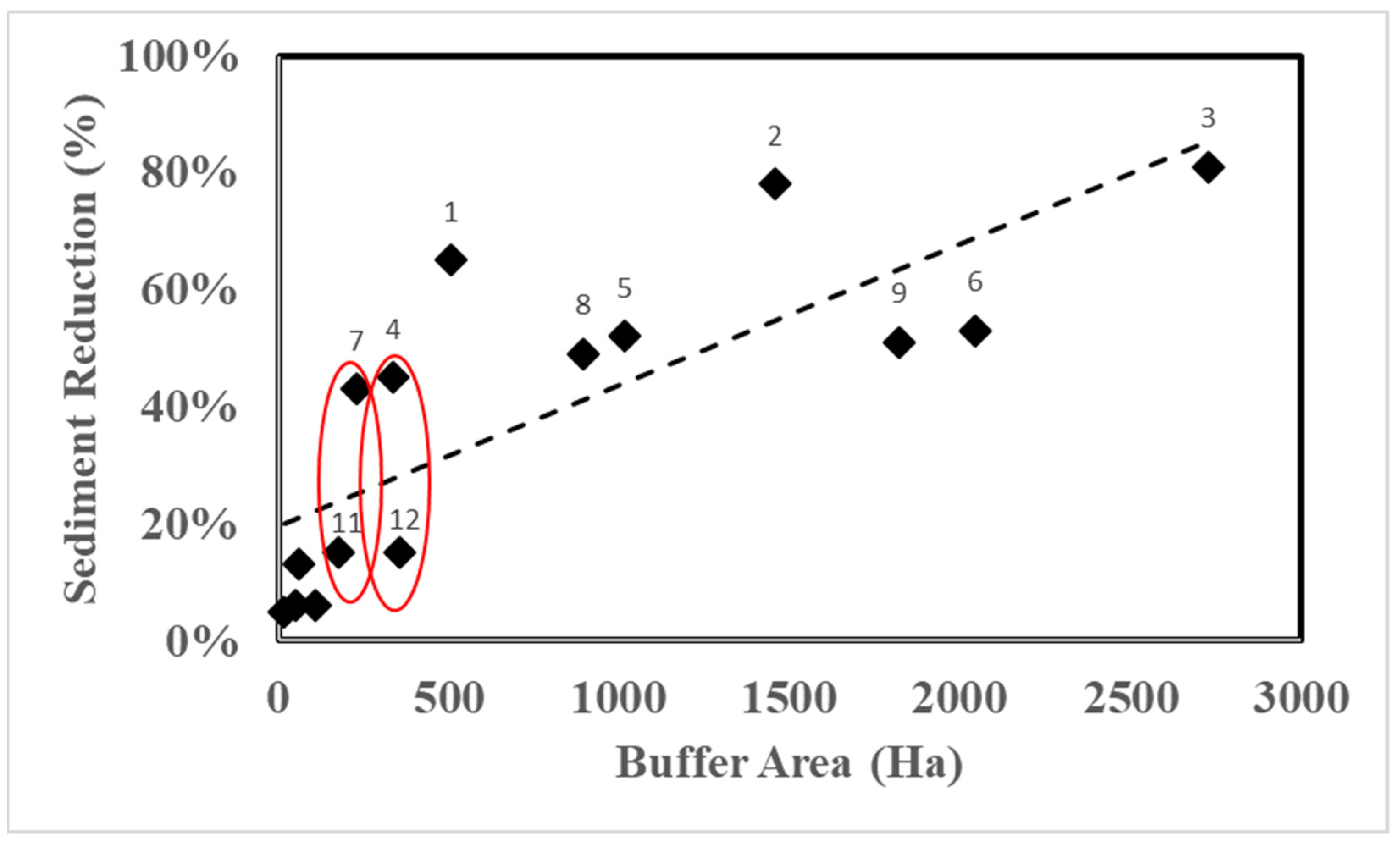
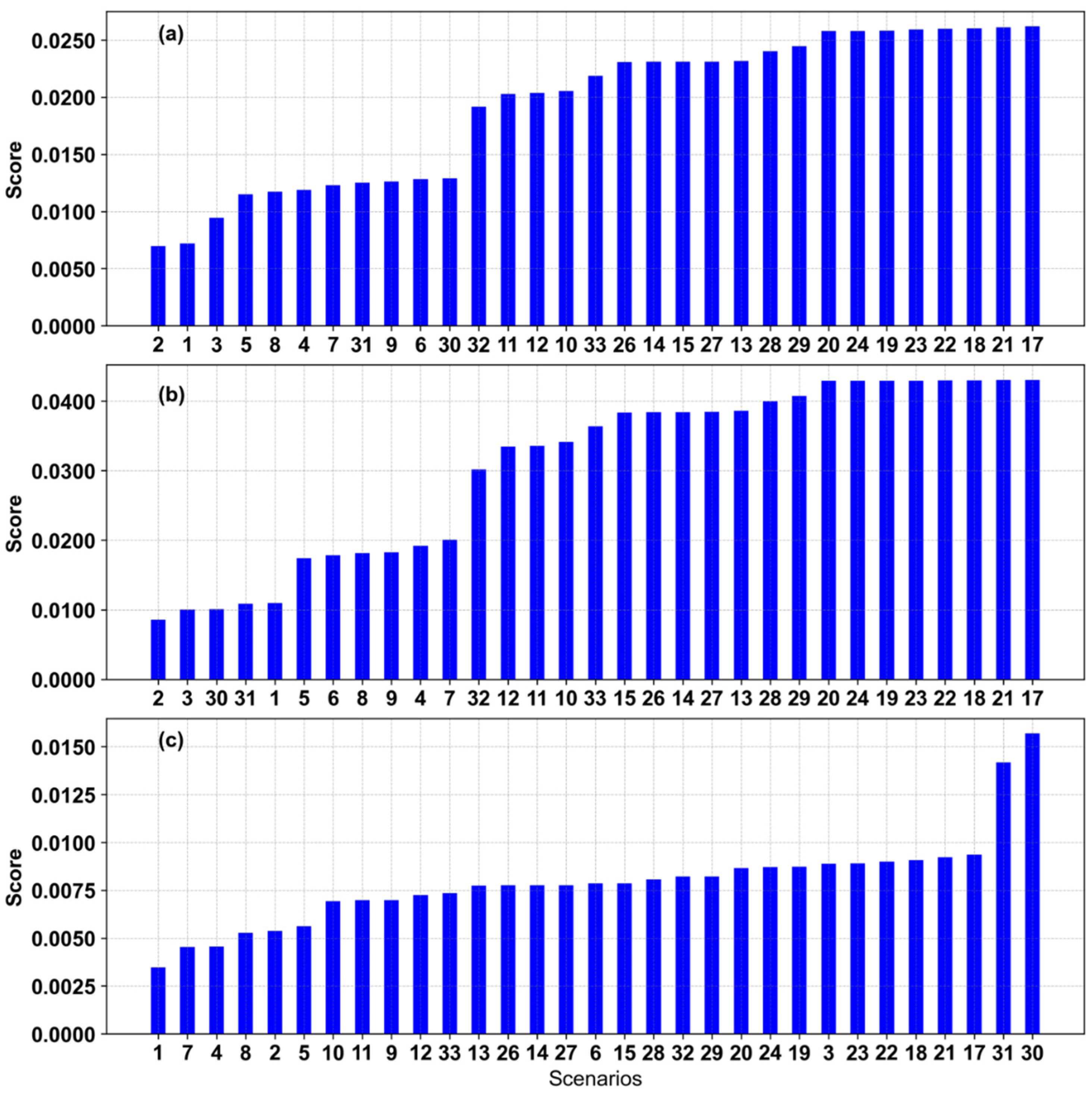
3.2. Conservation Practices Scenarios
4. Discussion
4.1. Prioritization of Conservation Practice Location
4.2. Optimization and Comparison of Conservation Practice Scenarios
4.3. Building Decision Support Tools Based on Study Results: A Riparian Buffer Example
4.4. Methodology Uncertainties
5. Conclusions
Author Contributions
Funding
Institutional Review Board Statement
Informed Consent Statement
Data Availability Statement
Acknowledgments
Conflicts of Interest
References
- Pimentel, D.; Harvey, C.; Resosudarmo, P.; Sinclair, K.; Kurz, D.; McNair, M.; Crist, S.; Shpritz, L.; Fitton, L.; Saffouri, R.; et al. Environmental and Economic Costs of Soil Erosion and Conservation Benefits. Science 1995, 267, 1117–1123. [Google Scholar] [CrossRef] [PubMed] [Green Version]
- Kagabo, D.M.; Stroosnijder, L.; Visser, S.M.; Moore, D. Soil Erosion, Soil Fertility and Crop Yield on Slow-Forming Terraces in the Highlands of Buberuka, Rwanda. Soil Tillage Res. 2013, 128, 23–29. [Google Scholar] [CrossRef]
- Zhuang, Y.; Du, C.; Zhang, L.; Du, Y.; Li, S. Research Trends and Hotspots in Soil Erosion from 1932 to 2013: A Literature Review. Scientometrics 2015, 105, 743–758. [Google Scholar] [CrossRef]
- Berihun, M.L.; Tsunekawa, A.; Haregeweyn, N.; Dile, Y.T.; Tsubo, M.; Fenta, A.A.; Meshesha, D.T.; Ebabu, K.; Sultan, D.; Srinivasan, R. Evaluating Runoff and Sediment Responses to Soil and Water Conservation Practices by Employing Alternative Modeling Approaches. Sci. Total Environ. 2020, 747, 141118. [Google Scholar] [CrossRef]
- Borrelli, P.; Robinson, D.A.; Panagos, P.; Lugato, E.; Yang, J.E.; Alewell, C.; Wuepper, D.; Montanarella, L.; Ballabio, C. Land Use and Climate Change Impacts on Global Soil Erosion by Water (2015–2070). Proc. Natl. Acad. Sci. USA 2020, 117, 21994–22001. [Google Scholar] [CrossRef] [PubMed]
- Eekhout, J.P.C.; de Vente, J. Global Impact of Climate Change on Soil Erosion and Potential for Adaptation through Soil Conservation. Earth Sci. Rev. 2022, 226, 103921. [Google Scholar] [CrossRef]
- Sulaeman, D.; Westhoff, T. The Causes and Effects of Soil Erosion, and How to Prevent It. Available online: https://www.wri.org/insights/causes-and-effects-soil-erosion-and-how-prevent-it (accessed on 15 September 2021).
- EPA. National Nonpoint Source Program: A Catalyst for Water Quality Improvements; EPA: Cincinnati, OH, USA, 2016.
- Jabbar, F.K.; Grote, K.; Tucker, R.E. A novel approach for assessing watershed susceptibility using weighted overlay and analytical hierarchy process (AHP) methodology: A case study in Eagle Creek Watershed, USA. Environ. Sci. Pollut. Res. 2019, 26, 31981–31997. [Google Scholar] [CrossRef] [Green Version]
- EPA. Basic Information about Nonpoint Source (NPS) Pollution. Available online: https://www.epa.gov/nps/basic-information-about-nonpoint-source-nps-pollution#:~:TEXT=NONPOINT%20SOURCE%20POLLUTION%20CAN%20INCLUDE,FOREST%20LANDS%2C%20AND%20ERODING%20STREAMBANKS (accessed on 8 August 2020).
- Arabi, M.; Frankenberger, J.R.; Engel, B.A.; Arnold, J.G. Representation of Agricultural Conservation Practices with SWAT. Hydrol. Process. 2008, 22, 3042–3055. [Google Scholar] [CrossRef]
- Kassam, A.; Friedrich, T.; Derpsch, R. Global Spread of Conservation Agriculture. Int. J. Environ. Stud. 2019, 76, 29–51. [Google Scholar] [CrossRef]
- Hermans, T.D.G.; Dougill, A.J.; Whitfield, S.; Peacock, C.L.; Eze, S.; Thierfelder, C. Combining Local Knowledge and Soil Science for Integrated Soil Health Assessments in Conservation Agriculture Systems. J. Environ. Manag. 2021, 286, 112192. [Google Scholar] [CrossRef]
- Farooq, M.; Siddique, K.H.M. Conservation Agriculture: Concepts, Brief History, and Impacts on Agricultural Systems; Springer International Publishing: Cham, Switzerland, 2015; pp. 3–17. [Google Scholar]
- USDA. Conservation Programs. Available online: https://www.ers.usda.gov/topics/natural-resources-environment/conservation-programs/#:~:text=Common%20practices%20include%20nutrient%20management,to%20exclude%20livestock%20from%20streams (accessed on 12 October 2021).
- Pittelkow, C.M.; Liang, X.; Linquist, B.A.; van Groenigen, K.J.; Lee, J.; Lundy, M.E.; van Gestel, N.; Six, J.; Venterea, R.T.; van Kessel, C. Productivity Limits and Potentials of The Principles of Conservation Agriculture. Nature 2015, 517, 365–368. [Google Scholar] [CrossRef]
- Brannan, K.M.; Mostaghimi, S.; McClellan, P.W.; Inamdar, S. Animalwaste Bmp Impacts on Sediment and Nutrient Losses in Runoff from the Owl Run Watershed. Trans. ASABE 2000, 43, 1155–1166. [Google Scholar] [CrossRef]
- Inamdar, S.P.; Mostaghimi, S.; McClellan, P.W.; Brannan, K.M. Bmp Impacts on Sediment and Nutrient Yields from an Agricultural Watershed in the Coastal Plain Region. Trans. ASABE 2001, 44, 1191–1200. [Google Scholar] [CrossRef] [Green Version]
- Richards, R.P.; Baker, D.B. Trends in Water Quality in LEASEQ Rivers and Streams (Northwestern Ohio), 1975–1995. J. Environ. Qual. 2002, 31, 90–96. [Google Scholar] [CrossRef]
- Gagnon, S.R.; Makuch, J.; Sherman, T.J. Implementing Agricultural Conservation Practices: Barriers and Incentives: A Conservation Effects Assessment Bibliography; Water Quality Information Center, National Agricultural Library: Beltsville, MD, USA, 2004.
- Gagnon, S.R.; Makuch, J.; Harper, C.Y. Effects of Agricultural Conservation Practices on Fish and Wildlife [Volume 2]: A Conservation Effects Assessment Bibliography; Water Quality Information Center, National Agricultural Library: Beltsville, MD, USA, 2008; Volume 7b.
- Osmond, D.; Meals, D.; Hoag, D.; Arabi, M.; Luloff, A.; Jennings, G.; McFarland, M.; Spooner, J.; Sharpley, A.; Line, D. Improving Conservation Practices Programming to Protect Water Quality in Agricultural Watersheds: Lessons Learned from the National Institute of Food and Agriculture–Conservation Effects Assessment Project. J. Soil Water Conserv. 2012, 67, 122A–127A. [Google Scholar] [CrossRef] [Green Version]
- Her, Y.; Chaubey, I.; Frankenberger, J.; Jeong, J. Implications of Spatial and Temporal Variations in Effects of Conservation Practices on Water Management Strategies. Agric. Water Manag. 2017, 180, 252–266. [Google Scholar] [CrossRef]
- Renschler, C.S.; Harbor, J. Soil Erosion Assessment Tools from Point to Regional Scales—The Role of Geomorphologists in Land Management Research and Implementation. Geomorphology 2002, 47, 189–209. [Google Scholar] [CrossRef]
- Gitau, M.W.; Veith, T.L.; Gburek, W.J.; Jarrett, A.R. Watershed Level Best Management Practice Selection and Placement in the Town Brook Watershed, New York. J. Am. Water Resour. Assoc. 2006, 42, 1565–1581. [Google Scholar] [CrossRef]
- Giri, S.; Nejadhashemi, A.P.; Woznicki, S.A. Evaluation of Targeting Methods for Implementation of Best Management Practices in the Saginaw River Watershed. J. Environ. Manag. 2012, 103, 24–40. [Google Scholar] [CrossRef]
- Xie, H.; Shen, Z.; Chen, L.; Qiu, J.; Dong, J. Time-Varying Sensitivity Analysis of Hydrologic and Sediment Parameters at Multiple Timescales: Implications for Conservation Practices. Sci. Total Environ. 2017, 598, 353–364. [Google Scholar] [CrossRef]
- Tomer, M.D.; Porter, S.A.; James, D.E.; Boomer, K.M.B.; Kostel, J.A.; McLellan, E. Combining Precision Conservation Technologies into A Flexible Framework to Facilitate Agricultural Watershed Planning. J. Soil Water Conserv. 2013, 68, 113A–120A. [Google Scholar] [CrossRef] [Green Version]
- Tomer, M.D.; Porter, S.A.; Boomer, K.M.B.; James, D.E.; Kostel, J.A.; Helmers, M.J.; Isenhart, T.M.; McLellan, E. Agricultural Conservation Planning Framework: 1. Developing Multipractice Watershed Planning Scenarios and Assessing Nutrient Reduction Potential. J. Environ. Qual. 2015, 44, 754–767. [Google Scholar] [CrossRef] [Green Version]
- Arnold, J.G.; Srinivasan, R.; Muttiah, R.S.; Williams, J.R. Large Area Hydrologic Modeling and Assessment Part I: Model Development. J. Am. Water Resour. Assoc. 1998, 34, 73–89. [Google Scholar] [CrossRef]
- Yuan, Y.; Koropeckyj-Cox, L. SWAT Model Application for Evaluating Agricultural Conservation Practice Effectiveness in Reducing Phosphorous Loss from the Western Lake Erie Basin. J. Environ. Manag. 2022, 302, 114000. [Google Scholar] [CrossRef] [PubMed]
- Naseri, F.; Azari, M.; Dastorani, M.T. Spatial Optimization of Soil and Water Conservation Practices Using Coupled SWAT Model and Evolutionary Algorithm. Int. Soil Water Conserv. Res. 2021, 9, 566–577. [Google Scholar] [CrossRef]
- Davie, D.K.; Lant, C.L. The effect of CRP enrollment on sediment loads in two southern Illinois streams. J. Soil Water Conserv. 1994, 49, 407–412. [Google Scholar]
- Carroll, C.; Halpin, M.; Burger, P.; Bell, K.; Sallaway, M.M.; Yule, D.F. The effect of crop type, crop rotation, and tillage practice on runoff and soil loss on a Vertisol in central Queensland. Aust. J. Soil Res. 1997, 35, 925–940. [Google Scholar] [CrossRef]
- Edwards, C.L.; Shannon, R.D.; Jarrett, A.R. Sedimentation Basin Retention Efficiencies for Sediment, Nitrogen, and Phosphorus from Simulated Agricultural Runoff. Trans. ASAE 1999, 42, 403–409. [Google Scholar] [CrossRef]
- Parkyn, S.M.; Davies-Colley, R.J.; Cooper, A.B.; Stroud, M.J. Predictions of stream nutrient and sediment yield changes following restoration of forested riparian buffers. Ecol. Eng. 2005, 24, 551–558. [Google Scholar] [CrossRef]
- Bailey, A.; Deasy, C.; Quinton, J.; Silgram, M.; Jackson, B.; Stevens, C. Determining the cost of in-field mitigation options to reduce sediment and phosphorus loss. Land Use Policy 2013, 30, 234–242. [Google Scholar] [CrossRef]
- Johnson, K.A.; Dalzell, B.J.; Donahue, M.; Gourevitch, J.; Johnson, D.L.; Karlovits, G.S.; Keeler, B.; Smith, J.T. Conservation Reserve Program (CRP) lands provide ecosystem service benefits that exceed land rental payment costs. Ecosyst. Serv. 2016, 18, 175–185. [Google Scholar] [CrossRef]
- Vigiak, O.; Malagó, A.; Bouraoui, F.; Grizzetti, B.; Weissteiner, C.J.; Pastori, M. Impact of current riparian land on sediment retention in the Danube River Basin. Sustain. Water Qual. Ecol. 2016, 8, 30–49. [Google Scholar] [CrossRef]
- Yuan, Y.; Locke, M.A.; Bingner, R.L. Annualized Agricultural Non-Point Source Model Application for Mississippi Delta Beasley Lake Watershed Conservation Practices Assessment. J. Soil Water Conserv. 2008, 63, 542–551. [Google Scholar] [CrossRef] [Green Version]
- Momm, H.G.; Porter, W.S.; Yasarer, L.M.; ElKadiri, R.; Bingner, R.L.; Aber, J.W. Crop Conversion Impacts on Runoff and Sediment Loads in The Upper Sunflower River Watershed. Agric. Water Manag. 2019, 217, 399–412. [Google Scholar] [CrossRef]
- Momm, H.G.; Yasarer, L.M.W.; Bingner, R.L.; Wells, R.R.; Kunhle, R.A. Evaluation of Sediment Load Reduction by Natural Riparian Vegetation in the Goodwin Creek Watershed. Trans. ASABE 2019, 62, 1325–1342. [Google Scholar] [CrossRef]
- Chahor, Y.; Casalí, J.; Giménez, R.; Bingner, R.L.; Campo, M.A.; Goñi, M. Evaluation of The Annagnps Model for Predicting Runoff and Sediment Yield in A Small Mediterranean Agricultural Watershed in Navarre (Spain). Agric. Water Manag. 2014, 134, 24–37. [Google Scholar] [CrossRef]
- Bisantino, T.; Bingner, R.; Chouaib, W.; Gentile, F.; Trisorio Liuzzi, G. Estimation of Runoff, Peak Discharge and Sediment Load at the Event Scale in a Medium-Size Mediterranean Watershed Using the Annagnps Model. Land Degrad. Dev. 2015, 26, 340–355. [Google Scholar] [CrossRef]
- Momm, H.G.; Bingner, R.L.; Emilaire, R.; Garbrecht, J.; Wells, R.R.; Kuhnle, R.A. Automated Watershed Subdivision for Simulations Using Multi-Objective Optimization. Hydrol. Sci. J. 2017, 62, 1564–1582. [Google Scholar] [CrossRef]
- Momm, H.G.; Bingner, R.L.; Yuan, Y.; Locke, M.A.; Wells, R.R. Spatial Characterization of Riparian Buffer Effects on Sediment Loads from Watershed Systems. J. Environ. Qual. 2014, 43, 1736–1753. [Google Scholar] [CrossRef]
- Bingner, R.L.; Theurer, F.D.; Yuan, Y.; Taguas, E.V. AnnAGNPS Technical Processes; U.S. Department of Agriculture: Washington, DC, USA, 2018.
- Momm, H.; Bingner, R.L.; Yuan, Y.; Kostel, J.; Monchak, J.J.; Locke, M.A.; Gilley, A. Characterization and Placement of Wetlands for Integrated Conservation Practice Planning. Trans. ASABE 2016, 59, 1345–1357. [Google Scholar] [CrossRef] [Green Version]
- Web Soil Survey, Natural Resources Conservation Service, United States Department of Agriculture. Available online: http://websoilsurvey.nrcs.usda.gov/ (accessed on 20 May 2020).
- Wagener, T.; Montanari, A. Convergence of Approaches toward Reducing Uncertainty in Predictions in Ungauged Basins. Water Resour. Res. 2011, 47. [Google Scholar] [CrossRef]
- TN Department of Finance and Administration. State of Tennessee LiDAR Initiative. Available online: https://lidar.tn.gov/ (accessed on 20 May 2020).
- Garbrecht, J.; Martz, L.W. Digital Landscape Parameterization for Hydrological Applications. IAHS Publ.-Ser. Proc. Rep.-Intern. Assoc. Hydrol. Sci. 1996, 235, 169–174. [Google Scholar]
- Garbrecht, J.; Martz, L.W. The Assignment of Drainage Direction Over Flat Surfaces in Raster Digital Elevation Models. J. Hydrol. 1997, 193, 204–213. [Google Scholar] [CrossRef]
- National Centers for Environmental Information, National Oceanic and Atmospheric Administration. Available online: https://www.ncdc.noaa.gov/cdo-web/search (accessed on 15 June 2020).
- NRCS. AGNPS Climate Generator GEM. Available online: https://www.nrcs.usda.gov/wps/portal/nrcs/detailfull/national/water/manage/hydrology/?cid=stelprdb1043533 (accessed on 15 June 2020).
- NRCS. Web Soil Survey. Available online: https://websoilsurvey.sc.egov.usda.gov/App/HomePage.htm (accessed on 19 June 2020).
- NRCS. Soil Data Access. Available online: https://sdmdataaccess.nrcs.usda.gov (accessed on 10 June 2020).
- NASS. National Agricultural Statistics Service. Available online: https://nassgeodata.gmu.edu/CropScape/ (accessed on 10 June 2020).
- Boryan, C.; Yang, Z.; Mueller, R.; Craig, M. Monitoring US agriculture: The US Department of Agriculture, National Agricultural Statistics Service, Cropland Data Layer Program. Geocarto Int. 2011, 26, 341–358. [Google Scholar] [CrossRef]
- U.S. National Agricultural Statistics Service. Available online: https://www.nass.usda.gov (accessed on 10 June 2020).
- USDA. Riparian Forest Buffers. Available online: https://www.fs.usda.gov/nac/practices/riparian-forest-buffers.php (accessed on 3 February 2020).
- Lv, J.; Wu, Y. Nitrogen Removal by Different Riparian Vegetation Buffer Strips with different Stand Densities and Widths. Water Supply 2021, 21, 3541–3556. [Google Scholar] [CrossRef]
- Mayer, P.M.; Reynolds, S.K.; McCutchen, M.D.; Canfield, T.J. Riparian Buffer Width, Vegetative Cover, and Nitrogen Removal Effectiveness: A Review of Current Science and Regulations; EPA: Cincinnati, OH, USA, 2005.
- Graziano, M.P.; Deguire, A.K.; Surasinghe, T.D. Riparian Buffers as a Critical Landscape Feature: Insights for Riverscape Conservation and Policy Renovations. Diversity 2022, 14, 172. [Google Scholar] [CrossRef]
- Lee, P.; Smyth, C.; Boutin, S. Quantitative review of riparian buffer width guidelines from Canada and the United States. J. Environ. Manag. 2004, 70, 165–180. [Google Scholar] [CrossRef]
- Clinton, B.D. Stream water responses to timber harvest: Riparian buffer width effectiveness. For. Ecol. Manag. 2011, 261, 979–988. [Google Scholar] [CrossRef]
- King, S.E.; Osmond, D.L.; Smith, J.; Burchell, M.R.; Dukes, M.; Evans, R.O.; Knies, S.; Kunickis, S. Effects of Riparian Buffer Vegetation and Width: A 12-Year Longitudinal Study. J. Environ. Qual. 2016, 45, 1243–1251. [Google Scholar] [CrossRef] [Green Version]
- Wenger, S. A Review of the Scientific Literature on Riparian Buffer Width, Extent, and Vegetation; Office of Public Service and Outreach, Institute of Ecology, The University of Georgia: Athens, GA, USA, 1999. [Google Scholar]
- Jones, R.S.; ElKadiri, R.; Momm, H. Canopy Classification Using LiDAR: A Generalizable Machine Learning Approach. Model. Earth Syst. Environ. 2022, 58, 1–14. [Google Scholar] [CrossRef]
- Zech, W.C.; Fang, X.; Logan, C. State-Of-The-Practice: Evaluation of Sediment Basin Design, Construction, Maintenance, and Inspection Procedures. Pract. Period. Struct. Des. Constr. 2014, 19. [Google Scholar] [CrossRef] [Green Version]
- Yasarer, L.M.W.; Bingner, R.L.; Momm, H.G. Characterizing Ponds in a Watershed Simulation and Evaluating Their Influence on Streamflow in a Mississippi Watershed. Hydrol. Sci. J. 2018, 63, 302–311. [Google Scholar] [CrossRef]
- Blanco, H.; Lal, R. Principles of Soil Conservation and Management; Springer: New York, NY, USA, 2008; Volume 167169. [Google Scholar]
- Gonzalez, J.M. Runoff and Losses of Nutrients and Herbicides Under Long-Term Conservation Practices (No-Till and Crop Rotation) in the U.S. Midwest: A Variable Intensity Simulated Rainfall Approach. Int. Soil Water Conserv. Res. 2018, 6, 265–274. [Google Scholar] [CrossRef]
- Shah, K.K.; Modi, B.; Pandey, H.P.; Subedi, A.; Aryal, G.; Pandey, M.; Shrestha, J. Diversified Crop Rotation: An Approach for Sustainable Agriculture Production. Adv. Agric. 2021, 2021, 8924087. [Google Scholar] [CrossRef]
- Shrestha, J.; Subedi, S.; Timsina, K.P.; Subedi, S.; Pandey, M.; Shrestha, A.; Shrestha, S.; Hossain, M.A. Sustainable Intensification in Agriculture: An Approach for Making Agriculture Greener and Productive. J. Nepal Agric. Res. Counc. 2021, 7, 133–150. [Google Scholar] [CrossRef]
- FAPRI-MU. Estimating Water Quality, Air Quality, and Soil Carbon Benefits of the Conservation Reserve Program; FAPRI-UMC Report #01-07; Food and Agriculture Policy Research Institute (FAPRI): Reno, NV, USA, 2007. [Google Scholar]
- Nagy-Reis, M.B.; Lewis, M.A.; Jensen, W.F.; Boyce, M.S. Conservation Reserve Program is a key element for managing white-tailed deer populations at multiple spatial scales. J. Environ. Manag. 2019, 248, 109299. [Google Scholar] [CrossRef]
- USDA. Conservation Reserve Program. Available online: https://www.fsa.usda.gov/programs-and-services/conservation-programs/conservation-reserve-program/ (accessed on 20 April 2020).
- Baginska, B.; Milne-Home, W.; Cornish, P.S. Modelling Nutrient Transport in Currency Creek, NSW with AnnAGNPS and PEST. Environ. Model. Softw. 2003, 18, 801–808. [Google Scholar] [CrossRef]
- Polyakov, V.; Fares, A.; Kubo, D.; Jacobi, J.; Smith, C. Evaluation of a Non-Point Source Pollution Model, AnnAGNPS, in a Tropical Watershed. Environ. Model. Softw. 2007, 22, 1617–1627. [Google Scholar] [CrossRef]
- Pease, L.M.; Oduor, P.; Padmanabhan, G. Estimating Sediment, Nitrogen, and Phosphorous Loads from the Pipestem Creek Watershed, North Dakota, Using AnnAGNPS. Comput. Geosci. 2010, 36, 282–291. [Google Scholar] [CrossRef]
- Taguas, E.V.; Yuan, Y.; Bingner, R.L.; Gómez, J.A. Modeling the Contribution of Ephemeral Gully Erosion Under Different Soil Managements: A Case Study in An Olive Orchard Microcatchment using the AnnAGNPS model. CATENA 2012, 98, 1–16. [Google Scholar] [CrossRef]
- Abdelwahab, O.; Bisantino, T.; Milillo, F.; Gentile, F. Runoff and Sediment Yield Modeling in A Medium-Size Mediterranean Watershed. J. Agric. Eng. 2013, 44. [Google Scholar] [CrossRef]
- Li, Z.; Luo, C.; Xi, Q.; Li, H.; Pan, J.; Zhou, Q.; Xiong, Z. Assessment of the AnnAGNPS model in Simulating Runoff and Nutrients in a Typical Small Watershed in The Taihu Lake Basin, China. CATENA 2015, 133, 349–361. [Google Scholar] [CrossRef]
- Nahkala, B.A.; Kaleita, A.L.; Soupir, M.L. Assessment of Input Parameters and Calibration Methods for Simulating Prairie Pothole Hydrology using AnnAGNPS. Appl. Eng. Agric. 2021, 37, 495–503. [Google Scholar] [CrossRef]
- Stroud Water Research Center. Model My Watershed. Available online: https://stroudcenter.org/virtual-learning-resource/model-my-watershed/ (accessed on 13 October 2020).
- Yuan, Y.; Bingner, R.L.; Locke, M.A. A review of effectiveness of vegetative buffers on sediment trapping in agricultural areas. Ecohydrology 2009, 2, 321–336. [Google Scholar] [CrossRef]
- Zhang, X.; Liu, X.; Zhang, M.; Dahlgren, R.A. A review of vegetated buffers and a meta-analysis of their mitigation efficacy in reducing nonpoint source pollution. J. Environ. Qual. 2010, 39, 76–84. [Google Scholar] [CrossRef] [PubMed] [Green Version]
- Hellerstein, D.M. The US Conservation Reserve Program: The Evolution of an Enrollment Mechanism. Land Use Policy 2017, 63, 601–610. [Google Scholar] [CrossRef]
- Taylor, M.R.; Hendricks, N.P.; Sampson, G.S.; Garr, D. The Opportunity Cost of the Conservation Reserve Program: A Kansas Land Example. Appl. Econ. Perspect. Policy 2021, 43, 849–865. [Google Scholar] [CrossRef]
- Palmeri, L.; Trepel, M. A GIS-Based Score System for Siting and Sizing of Created or Restored Wetlands: Two Case Studies. Water Resour. 2002, 16, 307–328. [Google Scholar] [CrossRef]
- Tanner, C.C.; Kadlec, R.H. Influence of Hydrological Regime on Wetland Attenuation of Diffuse Agricultural Nitrate Losses. Ecol. Eng. 2013, 56, 79–88. [Google Scholar] [CrossRef]
- USDA-NRCS. Mississippi River Basin Healthy Watersheds Initiative. Available online: https://www.nrcs.usda.gov/wps/portal/nrcs/detailfull/national/programs/initiatives/?cid=stelprdb1048200 (accessed on 5 February 2020).


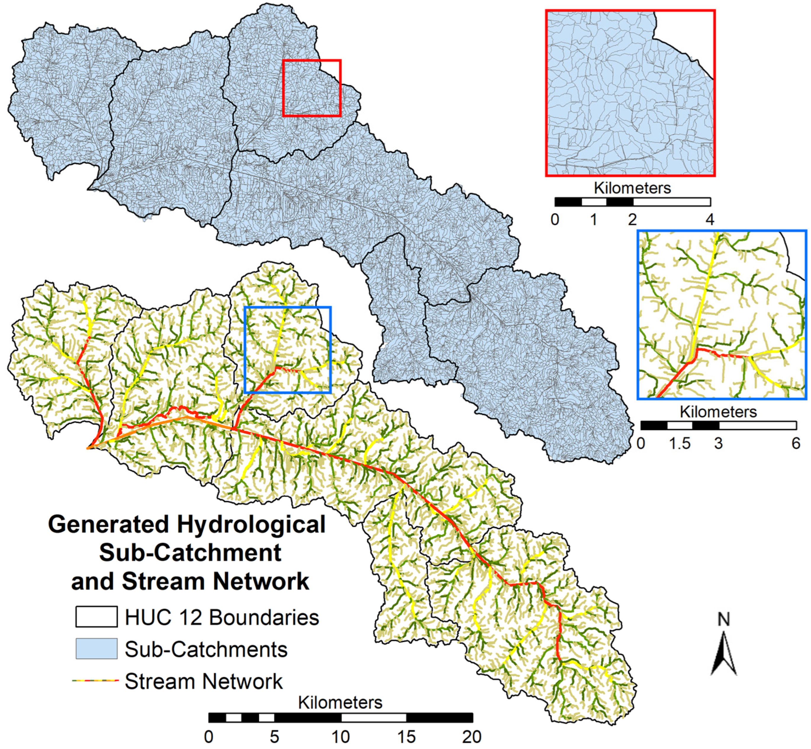
| HUC-12 Name | AnnAGNPS Cells (Sub-Catchments) | |||
|---|---|---|---|---|
| Number | Average Area (ha) | Average Slope (%) | Average Flow Length (m) | |
| North Fork Forked Deer River Upper | 2946 | 5.00 | 8% | 246.45 |
| Cain Creek | 904 | 4.81 | 8% | 245.89 |
| Mud Creek | 1682 | 5.04 | 6% | 255.84 |
| North Fork Forked Deer River Middle | 3165 | 5.10 | 5% | 259.92 |
| Doakville Creek | 1565 | 4.95 | 6% | 243.84 |
| North Fork Forked Deer River Lower | 2311 | 4.99 | 4% | 259.56 |
| Total | 12,573 | |||
| Crop | Date | Operation |
|---|---|---|
| Corn | 15 Mar. | Bedder/Lister |
| 1 Apr. | Disk | |
| 13 Apr. | Fertilizer | |
| 14 Apr. | Disk | |
| 15 Apr. | Sprayer | |
| 16 Apr. | Plant | |
| 9 May | Sprayer | |
| 15 May | Fertilizer | |
| 29 May | Sprayer | |
| 15 Sep. | Harvest | |
| 16 Sep. | Weed Growth | |
| Cotton | 17 Apr. | Sprayer |
| 18 Apr. | Fertilizer | |
| 1 May | Plant | |
| 15 May | Sprayer | |
| 15 June | Fertilizer | |
| 16 June | Sprayer | |
| 15 July | Sprayer | |
| 31 July | Sprayer | |
| 15 Aug. | Sprayer | |
| 29 Aug. | Defoliant | |
| 15 Oct. | Weed Growth | |
| Soybean | 20 Mar. | Chisel |
| 5 May | Fertilizer | |
| 10 May | Disk | |
| 11 May | Plant | |
| 29 May | Sprayer | |
| 20 July | Sprayer | |
| 28 Aug. | Sprayer | |
| 15 Oct. | Harvest | |
| 20 Oct. | Weed Growth |
| Crop | Date | Operation |
|---|---|---|
| Soybean (with no rotation) | 20 Mar. | Chisel |
| 5 May | Fertilizer | |
| 10 May | Disk | |
| 11 May | Plant | |
| 29 May | Sprayer | |
| 20 July | Sprayer | |
| 28 Aug. | Sprayer | |
| 15 Oct. | Harvest | |
| 20 Oct. | Weed Growth | |
| Winter Wheat + Soybean Rotation | 30 Oct. | Sprayer |
| 31 Oct. | Fertilizer | |
| 1 Nov. | Rill or Air Seeder | |
| 15 Nov. | Sprayer | |
| 15 Feb. | Fertilizer | |
| 15 Mar. | Sprayer | |
| 10 May | Disk | |
| 15 May | Sprayer | |
| 10 June | Harvest | |
| 11 June | Sprayer | |
| 13 June | Plant | |
| 27 June | Sprayer | |
| 20 July | Sprayer | |
| 28 Aug. | Sprayer | |
| 15 Oct. | Harvest | |
| 20 Oct. | Weed Growth |
| Simulation ID | Location Description | Riparian Buffer Width | Sediment Load (Mg/Year) | Sediment Reduction (%) | Spatial Footprint (Ha) |
|---|---|---|---|---|---|
| 1 | All Streams | 10 m | 71,312.7 | 65% | 506.6 |
| 2 | All Streams | 30 m | 44,970.2 | 78% | 1458.3 |
| 3 | All Streams | 60 m | 39,745.7 | 81% | 2728.2 |
| 4 | All streams adjacent to agricultural fields. | 10 m | 113,389.3 | 45% | 338.0 |
| 5 | All streams adjacent to agricultural fields. | 30 m | 99,602.6 | 52% | 1018.9 |
| 6 | All streams adjacent to agricultural fields. | 60 m | 96,321.7 | 53% | 2043.8 |
| 7 | All streams adjacent to agricultural fields with a sediment yield higher than 3.7 Mg/ha/year | 10 m | 118,246.5 | 43% | 228.6 |
| 8 | All streams adjacent to agricultural fields with a sediment yield higher than 3.7 Mg/ha/year | 30 m | 105,205.8 | 49% | 893.9 |
| 9 | All streams adjacent to agricultural fields with a sediment yield higher than 3.7 Mg/ha/year | 60 m | 101,905.8 | 51% | 1823.0 |
| 10 | All streams adjacent to agricultural fields with a sediment yield higher than 14.2 Mg/ha/year | 10 m | 178,229.7 | 13% | 60.9 |
| 11 | All streams adjacent to agricultural fields with a sediment yield higher than 14.2 Mg/ha/year | 30 m | 175,074.4 | 15% | 175.0 |
| 12 | All streams adjacent to agricultural fields with a sediment yield higher than 14.2 Mg/ha/year | 60 m | 174,124.0 | 15% | 357.9 |
| 13 | All streams adjacent to agricultural fields with a sediment yield higher than 19.4 Mg/ha/year | 10 m | 195,271.1 | 5% | 19.1 |
| 14 | All streams adjacent to agricultural fields with a sediment yield higher than 19.4 Mg/ha/year | 30 m | 194,101.3 | 6% | 52.7 |
| 15 | All streams adjacent to agricultural fields with a sediment yield higher than 19.4 Mg/ha/year | 60 m | 193,756.4 | 6% | 106.5 |
| 16 | Existing riparian buffer | Variable | 178,956.2 | 13% | 4683.8 |
| Baseline Conditions | No buffer is integrated into the model | 0 m | 205,880.2 | 0% | 0 |
| Simulation ID | Scenario Classification (Figure 6b) | Sediment Load (Mg/Year) | Sediment Reduction (%) | Spatial Footprint (Ha) |
|---|---|---|---|---|
| 17 | Class A | 10,699.1 | 95% | 214.3 |
| 18 | Class B | 70,137.00 | 66% | 200.7 |
| 19 | Class C | 184,607.9 | 10% | 91.2 |
| 20 | Class D | 199,254.0 | 3% | 39.9 |
| 21 | Class E | 164,705.5 | 20% | 252.1 |
| 22 | Class F | 179,666.4 | 13% | 276.4 |
| 23 | Class G | 179,073.7 | 13% | 172.2 |
| 24 | Class H | 198,661.2 | 4% | 79.6 |
| 25 | Existing Sediment Basins | 204,992.0 | 0% | 82.8 |
| Baseline conditions | 205,880.2 | 0% | 0 | |
| Simulation ID | Description | Sediment Load (Mg/year) | Sediment Reduction (%) | Spatial Footprint (Ha) |
|---|---|---|---|---|
| 26 | Crop rotation is applied to all soybean fields in the watershed | 182,278.4 | 11% | 0 * |
| 27 | Crop rotation is applied to all soybean fields in the watershed with a sediment yield higher than 3.7 Mg/ha/year | 193,476.4 | 11% | 0 * |
| 28 | Crop rotation is applied to all soybean fields in the watershed with a sediment yield higher than 14.2 Mg/ha/year | 182,969.3 | 6% | 0 * |
| 29 | Crop rotation is applied to all soybean fields in the watershed with a sediment yield higher than 19.4 Mg/ha/year | 197,905.3 | 4% | 0 * |
| Baseline Conditions | No additional crop rotation is integrated into the model | 205,880.2 | 0% | 0 * |
| Simulation ID | Description | Sediment Load (Mg/Year) | Sediment Reduction (%) | Spatial Footprint (Ha) |
|---|---|---|---|---|
| 30 | CRP is applied to all agricultural fields in the watershed | 38,598.1 | 81% | 7146.9 |
| 31 | CRP is applied to all agricultural fields in the watershed with a sediment yield higher than 3.7 Mg/ha/year | 44,460.2 | 78% | 6792.5 |
| 32 | CRP is applied to all agricultural fields in the watershed with a sediment yield higher than 14.2 Mg/ha/year | 154,930.8 | 25% | 1519.3 |
| 33 | CRP is applied to all agricultural fields in the watershed with a sediment yield higher than 19.4 Mg/ha/year | 186,290.7 | 10% | 388.5 |
| Baseline Conditions | No CRP is simulated in the model | 205,880.2 | 0% | 0 |
Disclaimer/Publisher’s Note: The statements, opinions and data contained in all publications are solely those of the individual author(s) and contributor(s) and not of MDPI and/or the editor(s). MDPI and/or the editor(s) disclaim responsibility for any injury to people or property resulting from any ideas, methods, instructions or products referred to in the content. |
© 2023 by the authors. Licensee MDPI, Basel, Switzerland. This article is an open access article distributed under the terms and conditions of the Creative Commons Attribution (CC BY) license (https://creativecommons.org/licenses/by/4.0/).
Share and Cite
ElKadiri, R.; Momm, H.G.; Bingner, R.L.; Moore, K. Spatial Optimization of Conservation Practices for Sediment Load Reduction in Ungauged Agricultural Watersheds. Soil Syst. 2023, 7, 4. https://doi.org/10.3390/soilsystems7010004
ElKadiri R, Momm HG, Bingner RL, Moore K. Spatial Optimization of Conservation Practices for Sediment Load Reduction in Ungauged Agricultural Watersheds. Soil Systems. 2023; 7(1):4. https://doi.org/10.3390/soilsystems7010004
Chicago/Turabian StyleElKadiri, Racha, Henrique G. Momm, Ronald L. Bingner, and Katy Moore. 2023. "Spatial Optimization of Conservation Practices for Sediment Load Reduction in Ungauged Agricultural Watersheds" Soil Systems 7, no. 1: 4. https://doi.org/10.3390/soilsystems7010004