


Historical Global Review of Acid-Volatile Sulfide Sediment Monitoring Data
Abstract
:1. Introduction
2. Materials and Methods
3. Results
3.1. General Overview
3.2. Waterbody Types
3.2.1. Streams/Creeks
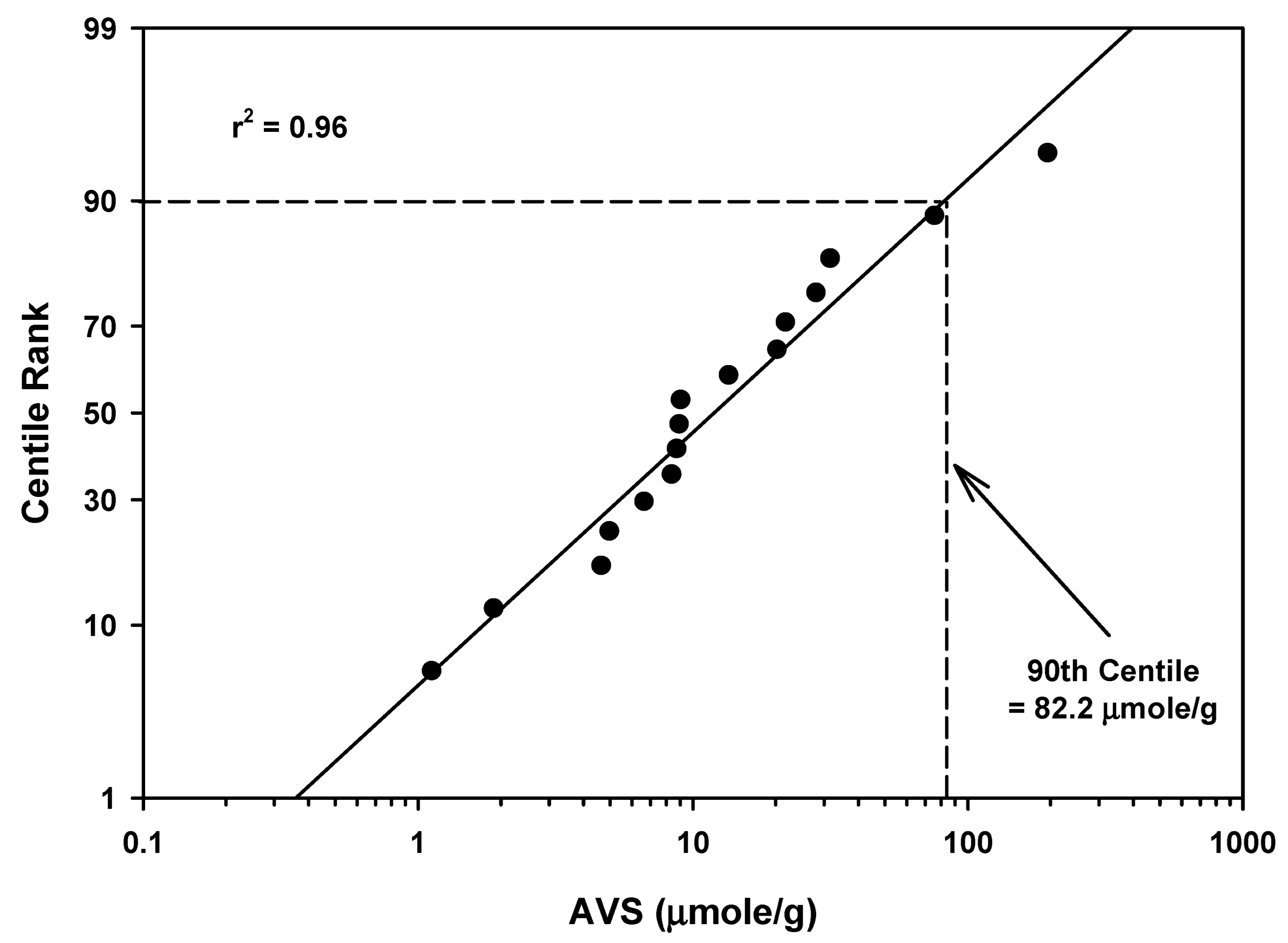
3.2.2. Rivers
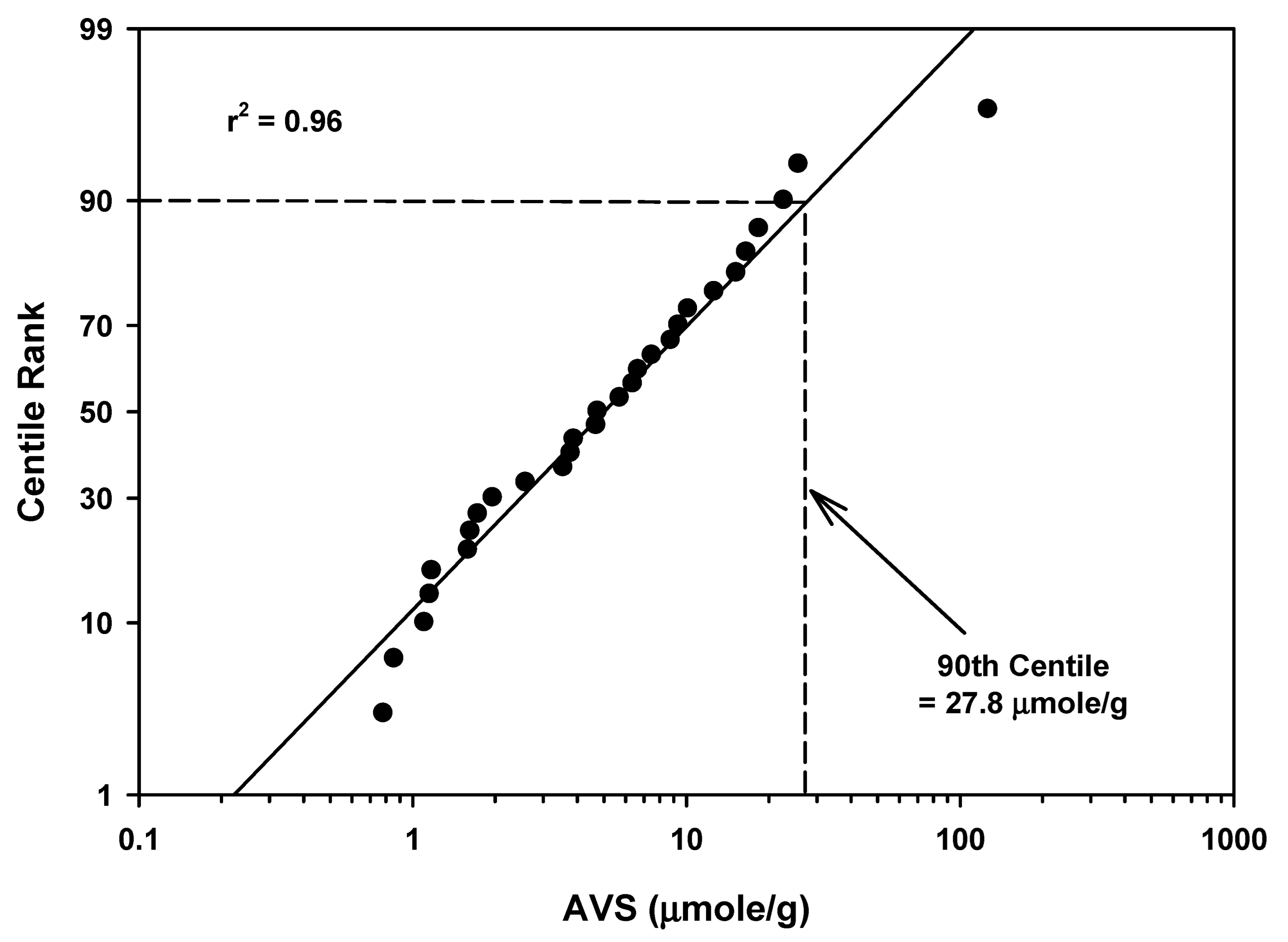
3.2.3. Lakes/Ponds/Reservoirs
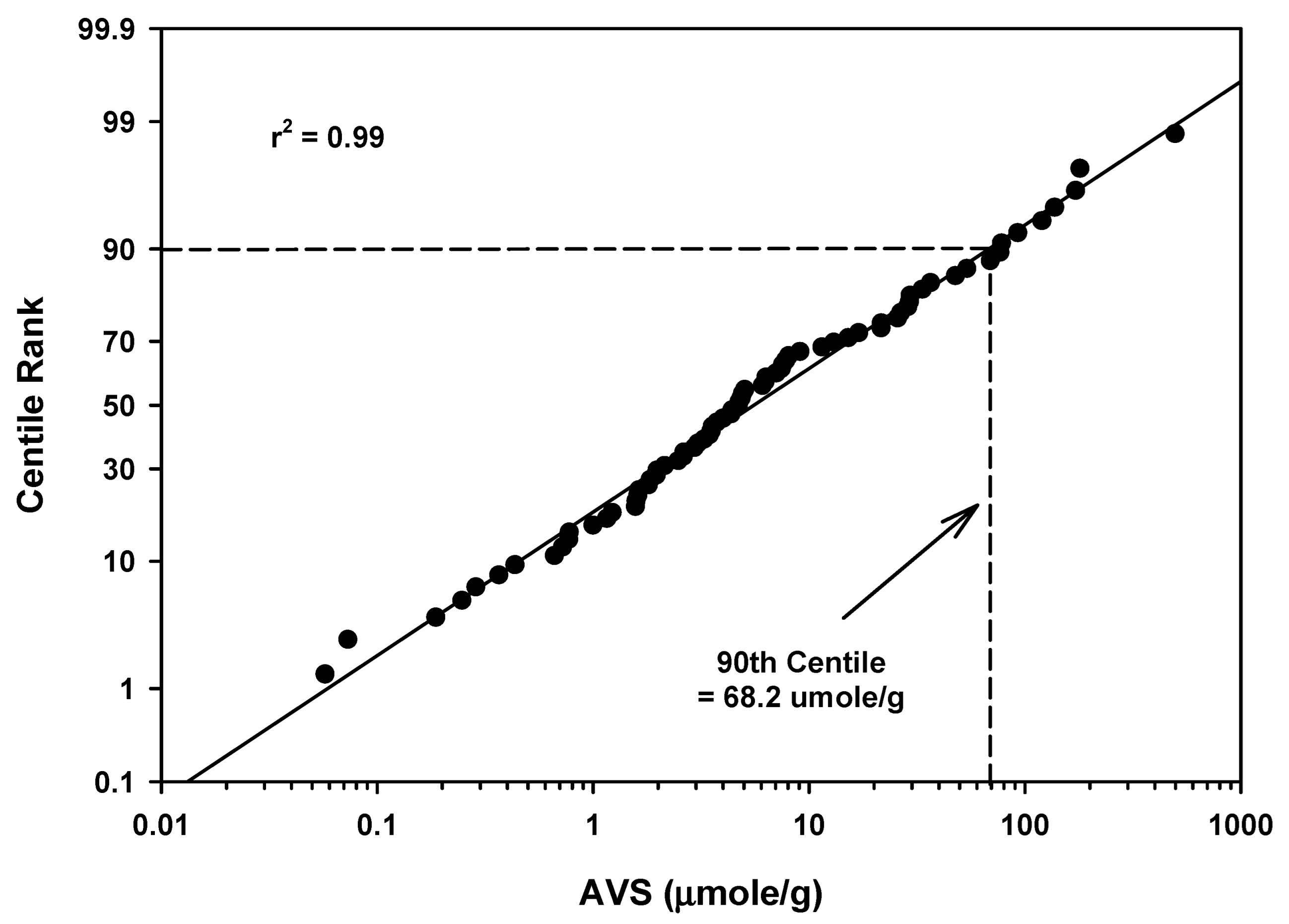
3.2.4. Estuarine/Marine Areas
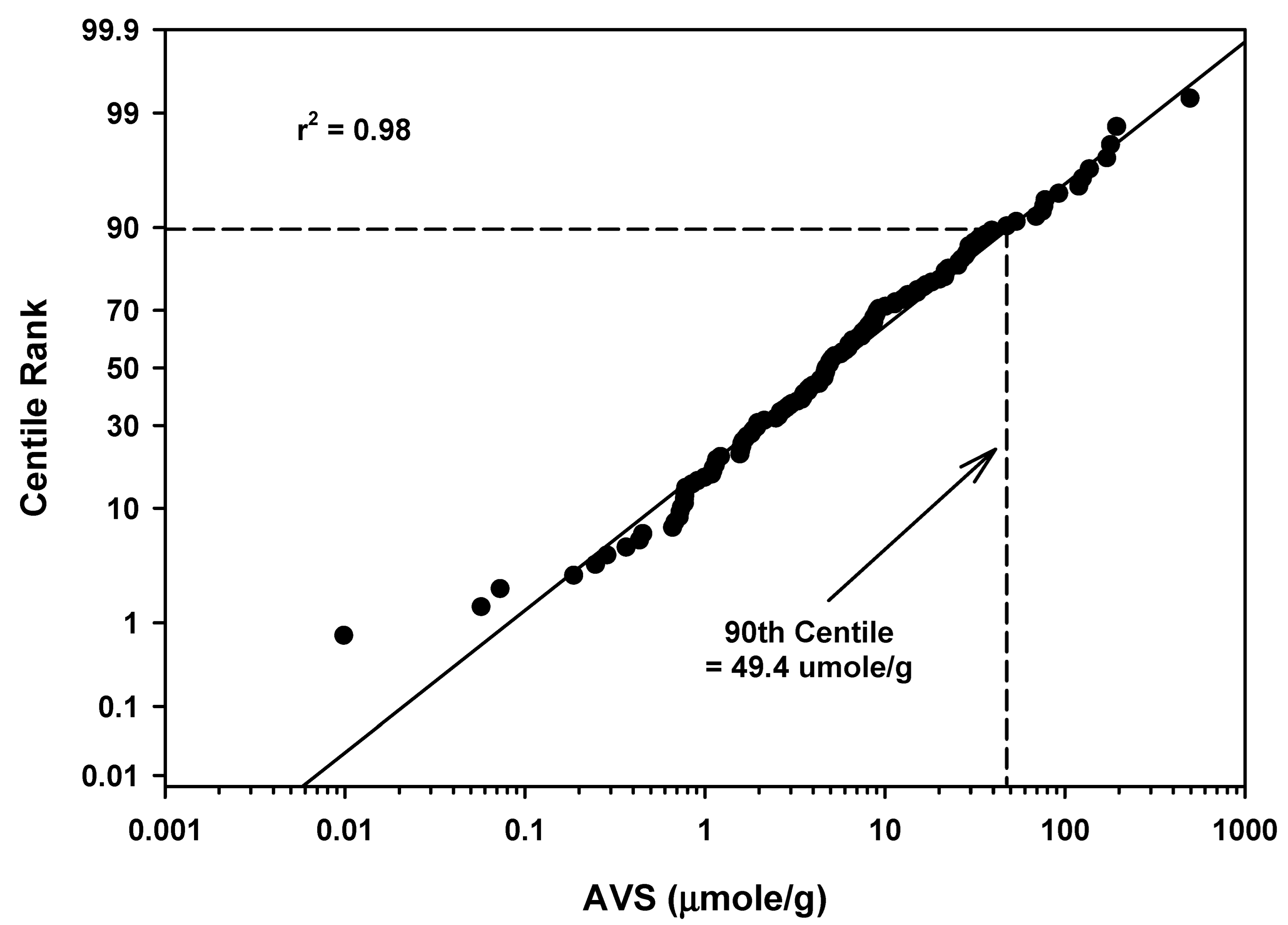
3.2.5. All Waterbodies
4. Discussion
5. Conclusions
Supplementary Materials
Author Contributions
Funding
Institutional Review Board Statement
Informed Consent Statement
Data Availability Statement
Acknowledgments
Conflicts of Interest
References
- Burton, G.A.; Green, A.; Baudo, R.; Forbes, V.; Nguyen, L.T.H.; Janssen, C.R.; Kukkonen, J.; Leppanen, M.; Maltby, L.; Soares, A.; et al. Characterizing sediment acid volatile sulfide concentrations in European Streams. Environ. Toxicol. Chem. 2007, 26, 1–12. [Google Scholar] [CrossRef] [PubMed]
- Rickard, D.; Morse, J.W. Acid volatile sulfides (AVS). Mar. Chem. 2005, 97, 141–197. [Google Scholar] [CrossRef]
- Di Toro, D.M.; Mahony, J.D.; Hansen, D.J.; Scott, K.J.; Hicks, M.B.; Mayr, S.M.; Redmond, M.S. Toxicity of cadmium in sediments: The role of acid volatile sulfide. Environ. Toxicol. Chem. 1990, 9, 1487–1502. [Google Scholar] [CrossRef]
- U. S. Environmental Protection Agency. Procedures for the Derivation of Equilibrium Partitioning Sediment Benchmarks (ESBs) for the Protection of Benthic Organism: Metal Mixtures (Cadmium, Copper, Lead, Nickel, Silver, and Zinc); Report EPA/600/R-02/011; Office of Research and Development: Washington, DC, USA, 2005.
- Morse, J.W.; Rickard, D. Chemical dynamics of sedimentary acid volatile sulfides. Environ. Sci. Technol. 2004, 38, 131–136. [Google Scholar] [CrossRef] [PubMed]
- Ulrich, G.A.; Martino, D.P.; Burger, K.; Routh, J.; Grossman, E.L.; Ammerman, J.W.; Suflita, J.M. Sulfur cycling in the terrestrial subsurface: Commensal interactions, spatial scales, and microbial heterogeneity. Microb. Ecol. 1998, 36, 141–151. [Google Scholar] [CrossRef]
- University of Auckland. Geology, Rocks and Minerals. Auckland, New Zealand. 2005. Available online: https://flexiblelearning.aukland.ac.nz/rocks_minerals/minerals/sulfur.html# (accessed on 15 May 2022).
- Gray, J.M.; Murphy, B.W. Parent Material and Soils—A Guide to the Influence of Parent Material on Soil Distribution in Eastern Australia; Technical Report 45 (Reprinted 2002); New South Wales Department of Land and Water Conservation: Sydney, WSW, Australia, 1999.
- Lander, L.; Reuther, R. Metals in Society and in the Environment: A Critical Review of Current Knowledge on Fluxes, Speciation, Bioavailability and Risk for Adverse Effects of Copper, Chromium, Nickel, and Zinc; Environmental Pollution Series; Kluwer Academic: Dordrecht, The Netherlands, 2004. [Google Scholar]
- Van Den Berg, G.A.; Loch, J.P.G.; Van Der Heijdt, L.M.; Zwolsman, J.J.G. Vertical distribution of acid-volatile sulfide and simultaneously extracted metals in a recent sedimentation area of the River Meuse in The Netherlands. Environ. Toxicol. Chem. 1998, 17, 758–763. [Google Scholar] [CrossRef]
- Leonard, E.N.; Mattson, V.R.; Benoit, D.A.; Hoke, R.A.; Ankley, G.T. Seasonal variation of acid volatile sulfide concentration in sediment cores from three northeastern Minnesota lakes. Hydrobiologia 1993, 271, 87–95. [Google Scholar] [CrossRef]
- Howard, D.E.; Evans, R.D. Acid-volatile sulfide (AVS) in a seasonally anoxic mesotrophic lake: Seasonal and spatial changes in sediment AVS. Environ. Toxicol. Chem. 1993, 12, 1051–1057. [Google Scholar] [CrossRef]
- Griethuysen, C.V.; Meijboom, E.W.; Koelmans, A.A. Spatial variation of metals and acid volatile sulfides in floodplain lake sediments. Environ. Toxicol. Chem. 2003, 22, 457–465. [Google Scholar] [CrossRef]
- Ankley, G.T.; Liber, K.; Call, D.J.; Markee, T.P.; Canfield, T.J.; Ingersoll, C.G. A field investigation of the relationship between zinc and acid volatile sulfide concentrations in freshwater sediments. J. Aquat. Ecosyst. Health 1996, 5, 255–264. [Google Scholar] [CrossRef]
- Carlson, A.R.; Phipps, G.L.; Mattson, V.R. The role of acid-volatile sulfide in determining cadmium bioavailability and toxicity in freshwater sediments. Environ. Toxicol. Chem. 1991, 10, 1309–1319. [Google Scholar] [CrossRef]
- Cervi, E.C.; Clark, S.; Boye, K.E.; Gustafsson, J.P.; Baken, S.; Burton, G.A., Jr. Copper transformation, speciation, and detoxification in anoxic and suboxic freshwater sediments. Chemosphere 2021, 282, 131063. [Google Scholar] [CrossRef] [PubMed]
- Hall, L.W., Jr.; Killen, W.D.; Anderson, R.D.; Alden, R.W., III. The influence of physical habitat, pyrethroids, and metals on benthic community condition in an urban and residential stream in California. Hum. Ecol. Risk Assess. 2009, 15, 526–553. [Google Scholar] [CrossRef]
- Hall, L.W., Jr.; Killen, W.D.; Anderson, R.D.; Alden, R.W., III. A three year assessment of the influence of physical habitat, pyrethroids and metals on benthic communities in two urban California streams. J. Ecosyst. Ecography 2013, 3, 133. [Google Scholar]
- Hall, L.W., Jr.; Killen, W.D.; Anderson, R.D.; Alden, R.W., III. The influence of multiple chemical and non-chemical stressors on benthic communities in a mid-west agricultural stream. J. Environ. Sci. Health Part A 2017, 52, 1008–1021. [Google Scholar] [CrossRef]
- Hall, L.W., Jr.; Anderson, R.D.; Killen, W.D.; Alden, R.W., III. An analysis of multiple stressors on resident benthic communities in a California agricultural stream. Air Soil Water Res. 2018, 11, 1–18. [Google Scholar] [CrossRef]
- Hall, L.W., Jr.; Killen, W.D.; Anderson, R.D.; Alden, R.W., III. Long term bioassessment multiple stressors study in a residential California stream. J. Environ. Sci. Health A 2021, 55, 346–360. [Google Scholar] [CrossRef]
- Poot, A.; Meerman, E.; Gillissen, F.; Koelmans, A.A. A kinetic approach to evaluate the association of acid volatile sulfide and simultaneously extracted metals in aquatic sediments. Environ. Toxicol. Chem. 2009, 28, 711–717. [Google Scholar] [CrossRef]
- Van Den Hoop, M.A.G.T.; Den Hollander, H.A.; Kerdijk, H.N. Spatial and seasonal variations of acid volatile sulphide (AVS) and simultaneously extracted metals (SEM) in Dutch marine and freshwater sediments. Chemosphere 1997, 35, 2307–2316. [Google Scholar] [CrossRef]
- Besser, J.M.; Kubitz, J.A.; Ingersoll, C.G.; Braselton, W.E.; Giesy, J.P. Influences on copper bioaccumulation, growth, and survival of the midge, Chironomus tentans, in metal-contaminated sediments. J. Aquat. Ecosyst. Health 1995, 4, 157–168. [Google Scholar] [CrossRef]
- Brumbaugh, W.G.; Ingersoll, C.G.; Kemble, N.E.; May, T.W.; Zajicek, J.L. Chemical characterization of sediments and pore water from the upper Clark Fork River and Milltown Reservoir, Montana. Environ. Toxicol. Chem. 1994, 13, 1971–1983. [Google Scholar] [CrossRef]
- De Jonge, M.; Dreesen, F.; De Paepe, J.; Blust, R.; Bervoets, L. Do Acid Volatile Sulfides (AVS) influence the accumulation of sediment-bound metals to benthic invertebrates under natural field conditions? Environ. Sci. Technol. 2009, 43, 4510–4516. [Google Scholar] [CrossRef] [PubMed]
- De Jonge, M.; Blust, R.; Bervoets, L. The relation between acid volatile sulfides (AVS) and metal accumulation in aquatic invertebrates: Implications of feeding behavior and ecology. Environ. Pollut. 2010, 158, 1381–1391. [Google Scholar] [CrossRef]
- Van Gheluwe, M.; Verdonck, F.; Van Sprang, P. Voluntary risk assessment of copper, copper II sulphate pentahydrate, copper(I)oxide, copper(II)oxide, dicopper chloride trihydroxide, Chapter 3: Environmental effects, Appendix O: Probabilistic assessment of copper bioavailability in sediments. In European Union Risk Assessment Report; European Union: Brussels, Belgium, 2008. [Google Scholar]
- Hall, L.W.; Killen, W.D.; Anderson, R.D.; Alden III, R.W. The relationship of benthic community metrics to pyrethroids, metals, and sediment characteristics in Cache Slough, California. J. Environ. Sci. Health A 2015, 51, 154–163. [Google Scholar] [CrossRef] [PubMed]
- Méndez-Fernández, L.; De Jonge, M.; Bervoets, L. Influences of sediment geochemistry on metal accumulation rates and toxicity in the aquatic oligochaete Tubifex tubifex. Aquat. Toxicol. 2014, 157, 109–119. [Google Scholar] [CrossRef] [PubMed]
- Naylor, C.; Davison, W.; Motelica-Heino, M.; Van Den Berg, G.A.; Van Der Heijdt, L.M. Potential kinetic availability of metals in sulphidic freshwater sediments. Sci. Total Environ. 2006, 357, 208–220. [Google Scholar] [CrossRef]
- Patton, G.W.; Crecelius, E.A. Simultaneously Extracted Metals/Acid-Volatile Sulfide and Total Metals in Surface Sediment from the Hanford Reach of the Columbia River and the Lower Snake River; U.S. Department of Energy, Pacific Northwest National Laboratory: Richland, WA, USA, 2001. Available online: http;//www.ntis.gov/ordering (accessed on 15 February 2022).
- Prica, M.; Dalmacija, B.; Rončević, S.; Krčmar, D.; Bečelić, M. A comparison of sediment quality results with acid volatile sulfide (AVS) and simultaneously extracted metals (SEM) ratio in Vojvodina (Serbia) sediments. Sci. Total Environ. 2008, 389, 235–244. [Google Scholar] [CrossRef]
- Ankley, G.T.; Mattson, V.R.; Leonard, E.N.; West, C.W.; Bennett, J.L. Predicting the acute toxicity of copper in freshwater sediments: Evaluation of the role of acid-volatile sulfide. Environ. Toxicol. Chem. 1993, 12, 315–320. [Google Scholar] [CrossRef]
- Allen, H.E.; Fu, G.; Deng, B. Analysis of acid-volatile sulfide (AVS) and simultaneously extracted metals (SEM) for the estimation of potential toxicity in aquatic sediments. Environ. Toxicol. Chem. 1993, 12, 1441–1453. [Google Scholar] [CrossRef]
- Huerta-Dlaz, M.A.; Carignan, R.; Tessier, A. Measurement of trace metals associated with acid volatile sulfides and pyrite in organic freshwater sediments. Environ. Sci. Technol. 1993, 27, 2367–2372. [Google Scholar] [CrossRef]
- Matisoff, G.; Berton Fisher, J.; McCall, P.L. Kinetics of nutrient and metal release from decomposing lake sediments. Geochim. Cosmochim. Acta 1981, 45, 2333–2347. [Google Scholar] [CrossRef]
- Sibley, P.K.; Ankley, G.T.; Cotter, A.M.; Leonard, E.N. Predicting chronic toxicity of sediments spiked with zinc: An evaluation of the acid-volatile sulfide model using a life-cycle test with the midge Chironomus tentans. Environ. Toxicol. Chem. 1996, 15, 2102–2112. [Google Scholar] [CrossRef]
- Van Den Berg, G.A.; Buykx, S.E.J.; Van Den Hoop, M.A.G.T.; Van Der Heijdt, L.M.; Zwolsman, J.J.G. Vertical profiles of trace metals and acid-volatile sulphide in a dynamic sedimentary environment: Lake Ketel, The Netherlands. Appl. Geochem. 2001, 16, 781–791. [Google Scholar] [CrossRef]
- Van Griethuysen, C.; De Lange, H.J.; Van Den Heuij, M.; De Bies, S.C.; Gillissen, F.; Koelmans, A.A. Temporal dynamics of AVS and SEM in sediment of shallow freshwater floodplain lakes. Appl. Geochem. 2006, 21, 632–642. [Google Scholar] [CrossRef]
- Yin, H.B.; Fan, C.X.; Ding, S.M.; Zhang, L.; Li, B. Acid volatile sulfides and simultaneously extracted metals in a metal-polluted area of Taihu Lake, China. Bull. Environ. Contam. Toxicol. 2008, 80, 351–355. [Google Scholar] [CrossRef]
- Zheng, L.; Xu, X.Q.; Xie, P. Seasonal and vertical distributions of acid volatile sulfide and metal bioavailability in a shallow, subtropical lake in China. Bull. Environ. Contam. Toxicol. 2004, 72, 326–334. [Google Scholar] [CrossRef]
- Alves, J.P.H.; Passos, E.A.; Garcia, C.A.B. Metals and acid volatile sulfide in sediment cores from the Sergipe River Estuary, northeast, Brazil. J. Braz. Chem. Soc. 2007, 18, 748–758. [Google Scholar] [CrossRef]
- Ankley, G.T.; Phipps, G.L.; Leonard, E.N.; Benoit, D.A.; Mattson, V.R.; Kosian, P.A.; Cotter, A.M.; Dierkes, J.R.; Hansen, D.J.; Mahony, J.D. Acid-volatile sulfide as a factor mediating cadmium and nickel bioavailability in contaminated sediments. Environ. Toxicol. Chem. 1991, 10, 1299–1307. [Google Scholar] [CrossRef]
- Arfaeinia, H.; Nabipour, I.; Ostovar, A.; Asadgol, Z.; Abuee, E.; Keshtkar, M.; Dobaradaran, S. Assessment of sediment quality based on acid-volatile sulfide and simultaneously extracted metals in heavily industrialized area of Asaluyeh, Persian Gulf: Concentrations, spatial distributions, and sediment bioavailability/toxicity. Environ. Sci. Pollut. Res. 2016, 23, 9871–9890. [Google Scholar] [CrossRef]
- Campana, O.; Rodríguez, A.; Blasco, J. Bioavailability of heavy metals in the Guadalete River Estuary (SW Iberian Peninsula). Cienc. Mar. 2005, 31, 135–147. [Google Scholar] [CrossRef]
- Campana, O.; Rodríguez, A.; Blasco, J. Identification of a potential toxic hot spot associated with AVS spatial and seasonal variation. Arch. Environ. Contam. Toxicol. 2009, 56, 416–425. [Google Scholar] [CrossRef] [PubMed]
- Chai, M.; Shen, X.; Li, R.; Qiu, G. The risk assessment of heavy metals in Futian mangrove forest sediment in Shenzhen Bay (South China) based on SEM-AVS analysis. Mar. Pollut. Bull. 2015, 97, 431–439. [Google Scholar] [CrossRef] [PubMed]
- Di Toro, D.M.; Mahony, J.D.; Hansen, D.J.; Scott, K.J.; Carlson, A.R.; Ankley, G.T. Acid volatile sulfide predicts the acute toxicity of cadmium and nickel in sediments. Environ. Sci. Technol. 1992, 26, 96–101. [Google Scholar] [CrossRef]
- Fang, T.; Li, X.; Zhang, G. Acid volatile sulfide and simultaneously extracted metals in the sediment cores of the Pearl River Estuary, South China. Ecotoxicol. Environ. Saf. 2005, 61, 420–431. [Google Scholar] [CrossRef]
- Gao, X.; Li, P.; Chen, C.T.A. Assessment of sediment quality in two important areas of mariculture in the Bohai Sea and the northern Yellow Sea based on acid-volatile sulfide and simultaneously extracted metal results. Mar. Pollut. Bull. 2013, 72, 281–288. [Google Scholar] [CrossRef] [PubMed]
- Hansen, D.J.; Berry, W.J.; Mahony, J.D.; Boothman, W.S.; Di Toro, D.M.; Robson, D.L.; Ankley, G.T.; Ma, D.; Yan, Q.; Pesch, C.E. Predicting the toxicity of metal-contaminated field sediments using interstitial concentration of metals and acid-volatile sulfide normalizations. Environ. Toxicol. Chem. 1996, 15, 2080–2094. [Google Scholar] [CrossRef]
- Hinkey, L.M.; Zaidi, B.R. Differences in SEM-AVS and ERM-ERL predictions of sediment impacts from metals in two US Virgin Islands marinas. Mar. Pollut. Bull. 2007, 54, 180–185. [Google Scholar] [CrossRef]
- Li, F.; Lin, J.Q.; Liang, Y.Y.; Gan, H.Y.; Zeng, X.Y.; Duan, Z.P.; Liang, K.; Liu, X.; Huo, Z.H.; Wu, C.H. Coastal surface sediment quality assessment in Leizhou Peninsula (South China Sea) based on SEM-AVS analysis. Mar. Pollut. Bull. 2014, 84, 424–436. [Google Scholar] [CrossRef]
- Li, L.; Xiaojing, W.; Jihua, L.; Xuefa, S.; Deyi, M. Assessing metal toxicity in sediments using the equilibrium partitioning model and empirical sediment quality guidelines: A case study in the nearshore zone of the Bohai Sea, China. Mar. Pollut. Bull. 2014, 85, 114–122. [Google Scholar] [CrossRef]
- Liu, J.; Yan, C.; Macnair, M.R.; Hu, J.; Li, Y. Vertical distribution of acid-volatile sulfide and simultaneously extracted metals in mangrove sediments from the Jiulong River Estuary, Fujian, China. Environ. Sci. Pollut. Res. 2007, 14, 345–349. [Google Scholar] [CrossRef]
- Jingchun, L.; Chongling, Y.; Spencer, K.L.; Ruifeng, Z.; Haoliang, L. The distribution of acid-volatile sulfide and simultaneously extracted metals in sediments from a mangrove forest and adjacent mudflat in Zhangjiang Estuary, China. Mar. Pollut. Bull. 2010, 60, 1209–1216. [Google Scholar] [CrossRef] [PubMed]
- Machado, W.; Carvalho, M.F.; Santelli, R.E.; Maddock, J.E.L. Reactive sulfides relationship with metals in sediments from an eutrophicated estuary in Southeast Brazil. Mar. Pollut. Bull. 2004, 49, 89–92. [Google Scholar] [CrossRef]
- Meyer, S.F.; Gersberg, R.M. Heavy metals and acid-volatile sulfides in sediments of the Tijuana Estuary. Bull. Environ. Contam. Toxicol. 1997, 59, 113–119. [Google Scholar] [CrossRef]
- Maryland Department of the Environment. Water Quality Analyses for Zinc in the Middle Harbor and Curtis Bay/Creek Portions of Patapsco River Mesohaline Chesapeake Bay Tidal Segment in Baltimore City, Baltimore County, and Anne Arundel County, Maryland; Watershed Protection Division: Baltimore, Maryland, 2022.
- Mucha, A.P.; Vasconcelos, M.T.S.D.; Bordalo, A.A. Spatial and seasonal variations of the macrobenthic community and metal contamination in the Douro estuary (Portugal). Mar. Environ. Res. 2005, 60, 531–550. [Google Scholar] [CrossRef]
- Nasr, S.M.; Khairy, M.A.; Okbah, M.A.; Soliman, N.F. AVS-SEM relationships and potential bioavailability of trace metals in sediments from the Southeastern Mediterranean Sea, Egypt. Chem. Ecol. 2014, 30, 15–28. [Google Scholar] [CrossRef]
- Nizoli, E.C.; Luiz-Silva, W. Seasonal AVS-SEM relationship in sediments and potential bioavailability of metals in industrialized estuary, southeastern Brazil. Environ. Geochem. Health 2012, 34, 263–272. [Google Scholar] [CrossRef]
- Pignotti, E.; Guerra, R.; Covelli, S.; Fabbri, E.; Dinelli, E. Sediment quality assessment in a coastal lagoon (Ravenna, NE Italy) based on SEM-AVS and sequential extraction procedure. Sci. Total Environ. 2018, 635, 216–227. [Google Scholar] [CrossRef] [PubMed]
- Remaili, T.M.; Yin, N.; Bennett, W.W.; Simpson, S.L.; Jolley, D.F.; Welsh, D.T. Contrasting effects of bioturbation on metal toxicity of contaminated sediments results in misleading interpretation of the AVS-SEM metal-sulfide paradigm. Environ. Sci. Processes Impacts. 2018, 20, 1285–1296. [Google Scholar] [CrossRef]
- Shyleshchandran, M.N.; Mohan, M.; Ramasamy, E.V. Risk assessment of heavy metals in Vembanad Lake sediments (south-west coast of India), based on acid-volatile sulfide (AVS)-simultaneously extracted metal (SEM) approach. Environ. Sci. Pollut. Res. 2018, 25, 7333–7345. [Google Scholar] [CrossRef]
- Silva, J.B., Jr.; Nascimento, R.A.; de Oliva, S.T.; de Oliveira, O.M.C.; Ferreira, S.L.C. Bioavailability assessment of toxic metals using the technique “acid-volatile sulfide (AVS)-simultaneously extracted metals (SEM)” in marine sediments collected in Todos os Santos Bay, Brazil. Environ. Monit. Assess. 2016, 188, 544–554. [Google Scholar]
- Simpson, S.L. A rapid screening method for acid-volatile sulfide in sediments. Environ. Toxicol. Chem. 2001, 20, 2657–2661. [Google Scholar] [CrossRef] [PubMed]
- Wang, Z.; Yin, L.; Qin, X.; Wang, S. Integrated assessment of sediment quality in a coastal lagoon (Maluan Bay, China) based on AVS-SEM and multivariate statistical analysis. Mar. Pollut. Bull. 2019, 146, 476–487. [Google Scholar] [CrossRef] [PubMed]
- Yang, Y.; Zhang, L.; Chen, F.; Kang, M.; Wu, S.; Liu, J. Seasonal variation of acid volatile sulfide and simultaneously extracted metals in sediment cores from the Pearl River Estuary. Soil Sediment Contam. 2014, 23, 480–496. [Google Scholar] [CrossRef]
- Younis, A.M.; El-Zokm, G.M.; Okbah, M.A. Spatial variation of acid-volatile sulfide and simultaneously extracted metals in Egyptian Mediterranean Sea lagoon sediments. Environ. Monit. Assess. 2014, 186, 3567–3579. [Google Scholar] [CrossRef]
- Yu, K.C.; Tsai, L.J.; Chen, S.H.; Ho, S.T. Chemical binding of heavy metals in anoxic river sediments. Water Res. 2001, 35, 4086–4094. [Google Scholar] [CrossRef]
- Zhuang, W.; Gao, X. Acid-volatile sulfide and simultaneously extracted metals in surface sediments of the southwestern coastal Laizhou Bay, Bohai Sea: Concentrations, spatial distributions and the indication of heavy metal pollution status. Mar. Pollut. Bull. 2013, 76, 128–138. [Google Scholar] [CrossRef] [PubMed]
- Food and Agricultural Organization of the United Nations (FAO); United Nations Education Scientific and Cultural Organization (UNESCO). Soil Map of the World; FAO & UNESCO: Paris, France, 1972; Available online: https://www.fao.org/soils-portal/data-hub/soil-maps-and-databases/faounesco-soil-map-of-the-world/en/ (accessed on 2 June 2022).
- Olson, D.M.; Dinerstein, E.; Wikramanayake, E.D.; Burgess, N.D.; Powell, G.V.N.; Underwood, E.C.; D’Amico, J.A.; Itoua, I.; Strand, H.E.; Morrison, J.C.; et al. Terrestrial ecoregions of the world: A new map of life on earth. Bioscience 2001, 51, 933–938. [Google Scholar] [CrossRef]
- University of California Museum of Paleontology. The Worlds Biomes. University of California at Berkeley. 1996. Available online: www.ucmp.berkley.edu (accessed on 17 May 2022).
- SigmaPlot (SYSTAT). Available online: www.systat.com (accessed on 1 July 2022).
- Available online: https://www.britannica.com/science/Luvisol (accessed on 19 July 2022).
- Tsolova, W.; Kolchakova, V.; Zhiyanski, M. Carbon, nitrogen, and sulphur pools and fluxes in pyrite containing reclaimed soils (Technosols) at Gabra Village, Bularia. Environ. Processes 2014, 1, 405–414. [Google Scholar] [CrossRef] [Green Version]
- Available online: www.ecologypocketguide.com/temperate-broadleaf-and-mixed-forest (accessed on 19 July 2022).


| Location | Water Body/Type | Soil Type a | Biome Type | Depositional Areas Targeted? | # of Sites Sampled & Frequency | AVS (µmole/g) (Min-Max, Mean) | References |
|---|---|---|---|---|---|---|---|
| SW Missouri, USA | Turkey Creek, (ag/urban stream) | Acrisols | Temperate Broadleaf and Mixed Forest | Yes | Six sites sampled twice in one year (0–3 cm depth) | 6 sites, Mar 1995: (1.93–33.2, 11.5) b 6 sites, Jun 1995: (1.03–2.85, 1.70) b | [14] |
| Sweden | SW Sweden/Wadable | Cambisols/Podzols | Temperate Broadleaf and Mixed Forest | Yes | 3 sites | : (0.004–2.07, 0.693) | |
| Denmark | E Denmark/Wadable | Cambisols/Luvisols | Temperate Broadleaf and Mixed Forest | Yes | 6 sites | (0.058–1.69, 0.739) | |
| England | S England & Wales/Wadable | Gleysols/Cambisols/Luvisols | Temperate Broadleaf and Mixed Forest | Yes | 16 sites | : (0.007–31.5, 4.38) | |
| Finland | S Finland/Wadable | Podzols/Histosols | Boreal Forests/Taiga | Yes | 5 sites | (0.004–3.18, 0.928) | [1] c |
| Belgium | S Belgium/Wadable | Cambisols | Temperate Broadleaf and Mixed Forest | Yes | 6 sites | (0.020–44.0, 8.23) | |
| France | N France/Wadable | Luvisols/Cambisols/Podzols | Temperate Broadleaf and Mixed Forest | Yes | 12 sites | : (0.004–25.3, 5.21) | |
| Germany | W & S Germany/Wadable | Cambisols/Luvisols/Rendzinas | Temperate Broadleaf and Mixed Forest | Yes | 9 sites | (0.007–5.08, 0.795) | |
| Italy | N Italy/Wadable | NA d | NA d | Yes | 2 sites | (0.008–0.012, 0.010) | Burton et al. [1]c |
| E Wisconsin, USA | East River (ag stream) | Luvisols | Temperate Grasslands, Savannas and Shrublands | Not reported | 1 site sampled once e | 1 site: (mean = 8.8) | [15] |
| S Michigan, USA | River Raisin (rural stream) | Luvisols | Temperate Broadleaf and Mixed Forest | Not reported | 1 site sampled once (0–10 cm depth) | 1 site: (mean = 1.12) | [16] |
| Pittsburg, California, USA | Kirker Creek, small mostly urban creek | Luvisols | Mediterranean Forests, Woodlands, and Scrub | Yes | 14 sites with composite samples collected once for 2 years | 14 Sites: (0.071–23.7, 5.34) | [17] |
| Sacramento, California, USA | Arcade Creek/Urban creek | Luvisols | Temperate Grasslands, Savannas and Shrublands | Yes | 11 sites with composite samples collected once/year for 3 years | Arcade Sites: (0.012–3.92, 0.751) | [18] |
| Salinas, California, USA | Alisal, Gabilon and Natividad Creeks/Urban with some ag | Mediterranean Forests, Woodlands, and Scrub | 13 sites with composite samples collected once/year for 3 years | Salinas sites: (0.019–2.10, 0.781) | |||
| N Illinois, USA | Big Bureau Creek (ag stream) | Phaeozems | Temperate Grasslands, Savannas and Shrublands | Yes | 12 sites with composite samples collected once/year for 3 years | Sites 1–12: (0.230–1.19, 0.458) | [19] |
| Santa Maria, California, USA | Santa Maria River, Osco Flaco Creek, Orcutt Creek/(intensive ag) | Luvisols | Mediterranean Forests, Woodlands, and Scrub | Yes | 12 sites with composite samples collected once/year for 3 years | Sites 1–12 (0.07–25.8, 5.91) | [20] |
| Roseville / Pleasant Grove, California, USA | Upper Pleasant Grove Creek/(urban stream) Lower Pleasant Grove Creek/(ag creek) | Luvisols Fluvisols | Mediterranean Forests, Woodlands, and Scrub | Yes | 21 sites with composite samples collected once/year for 10 years | 18 Urban Sites: (0.028–12.4, 2.78) 3 Agricultural Sites: (3.08–5.68, 4.65) | [21] |
| SE Netherlands | Beekloop/Headwater stream | Podzols | Temperate Broadleaf and Mixed Forest | Not reported | 4 sites sampled once with 3 replicates per site | Sites L1–4: (13.1–62.6, 39.8) | [22] |
| N Netherlands | Freshwater Stream | Fluvisols | Temperate Broadleaf and Mixed Forest | Not reported | 1 site sampled once or monthly for a year | Freshwater stream: (0.657–7.64, 2.89) b | [23] |
| Location | Water Body/Type | Soil Type a | Ecoregion | Depositional Areas Targeted? | # of Sites Sampled & Frequency | AVS (µmole/g) (Min-Max, Mean) | References |
|---|---|---|---|---|---|---|---|
| W Montana, USA | Upper Clark Fork River & reference trib/(mountain river with ag & urban zones) | Luvisols/Kastanozems | Temperate Grasslands, Savannas and Shrublands | Not reported | 1 reference & 5 additional sites sampled once from composite grab samples in Aug 1993 (0–6 cm depth) | RC (reference): (mean = 1.9) Upper Clark Fork:(0.5–22.0, 8.8) | [24] |
| W Montana, USA b | Upper Clark Fork River & reference trib/(mountain river with ag & urban zones) | Luvisols/Kastanozems | Temperate Grasslands, Savannas and Shrublands | Yes | 1 reference & 5 additional sites sampled once from grab samples in Sep 1991 (0–6 cm depth) | CF06 (reference): (mean = 6.7) Upper Clark Fork:(0.3–19.1, 9.1) | [25] |
| N Belgium, E of Antwerp | Lowland riverine sediments | Podzols/Podzoluvisols | Temperate Broadleaf and Mixed Forest | Not reported | 17 sample sites (3 replicates each) sampled once | Sites 1–17: (0.763–205, 76.3) | [26] |
| N Belgium, Flanders Region | Lowland riverine sediments | Podzols/Podzoluvisols/Luvisols | Temperate Broadleaf and Mixed Forest | Not reported | 28 sample sites (3 replicates each) sampled once | Sites 1–28: (0.004–357, 28.3) | [27] |
| Flanders Region, N Belgium | Rivers Scheldt, Dender, Leie, & IJzer c | Podzols/Podzoluvisols/Luvisols/Fluvisols/Regosols | Temperate Broadleaf and Mixed Forest | Not reported | 44 sites sampled once | 44 Sites: (2.28–132, 31.8) | [28] |
| Rio Vista California, USA | Cache Slough/Tidal freshwater river | Fluvisols/Luvisols | Temperate Grasslands, Savannas and Shrublands | Yes | 12 sites with composite samples sampled twice a year for 3 years | 12 sites: (0.40–2.14, 1.13) | [29] |
| N Belgium | Nete/Scheldt River Basins/Lowland riverine sediments | Podzols/Podzoluvisols/Luvisols | Temperate Broadleaf and Mixed Forest | Not reported | 3 sites sampled once | 3 Sites: (24.9–321.3, 196.8) | [30] |
| S Netherlands | Meuse & Rhine Rivers confluence delta (agr/urban) | Fluvisols | Temperate Broadleaf and Mixed Forest | Not reported | 1 core sample for AVS (top 0–9 cm) | 1 core: (1.49–7.06, 5.01) d | [31] |
| Washington State, USA | Hanford Reach/Columbia River | Regosols | Deserts and Xeric Shrublands | Not reported | 4 sites sampled 2–3 times over 3 years | Hanford Reach Sites: (0.32–12.6, 4.68) | [32] |
| N Serbia | Various rivers & canals | Chernozems/Fluvisols/Phaeozems | Temperate Broadleaf and Mixed Forest | Yes | 12 sites sampled once in the spring 11 of the same sites sampled in the summer | Spring: (3.10–14.1, 8.43) Summer: (3.19–16.0, 9.00) | [33] |
| SW Netherlands | Meuse/Rhine River Delta (freshwater) | Fluvisols | Temperate Broadleaf and Mixed Forest | Yes | 4 sites sampled twice in Nov 1995 and once in Jun 1996 | Sites 1–4, Nov 1995: (7.4–52.5, 21.9) Sites 1–4, Jun 1996: (7.2–28.6, 13.6) | [10] |
| Netherlands | Kromme River (freshwater) | Fluvisols | Temperate Broadleaf and Mixed Forest | Not reported | 1 site sampled monthly for a year (0–10 cm depth) | Kromme River: (6.87–38.4, 20.4) d | [23] |
| Location | Water Body/Type | Soil Type a | Predominate Biome Type | Depositional Areas Targeted? | # of Sites Sampled & Frequency | AVS (µmoles/g) (Min-Max, Mean) | References |
|---|---|---|---|---|---|---|---|
| Washington State, USA | Steilacoom Lake/Urban recreational lake | Cambisols | Temperate Coniferous Forest | Not reported | 11 sites with measured concentrations sampled once | Steilacoom Lake: (0.30–4.16, 1.97) | [34] |
| NE Minnesota, USA | Fish Lake, Caribou Lake, and Pike Lake | Podzoluvisols | Temperate Broadleaf and Mixed Forest | Not reported | 3 sites sampled once and analyzed with 3–4 different methods/labs | Fish Lake: (1.3–1.87, 1.63) Caribou Lake: (5.35–8.4, 6.40) Pike Lake: (16.51–16.74, 16.6) | [35] |
| W Montana, USA | Milltown Reservoir in Clark Fork River System | Milltown Reservoir: Luvisols | Temperate Grasslands, Savannas and Shrublands | 6 sites sampled once from composited grabs (0–6 cm depth) | Milltown Reservoir: (0.2–47.0, 18.5) | ||
| Michigan, USA | Primarily lake sites in the upper peninsula of Michigan | Upper Peninsula: Podzols/Histosols | Temperate Broadleaf and Mixed Forest | Not reported | 8 sites sampled once from composited grabs (0–6 cm depth) | Upper Peninsula: (0.1–65.0, 10.2) | [24] |
| W Michigan, USA | Primarily lake sites in the lower peninsula of Michigan | Lower Peninsula: Luvisols/Podzols/Histosols | Temperate Broadleaf and Mixed Forest | 8 sites sampled once from composited grabs (0–6 cm depth) | Lower Peninsula: (14.0–471.0, 127.1) | ||
| W Montana, USA b | Milltown Reservoir in Clark Fork River System | Luvisols | Temperate Grasslands, Savannas and Shrublands | Yes | 6 sites sampled once from composited grabs (0–6 cm depth) | Milltown Reservoir: (0.6–23.3, 9.4) | [25] |
| NE Minnesota, USA | Pequaywan & West Bearskin Lakes (large, isolated lakes) | Podzoluvisols | Temperate Broadleaf and Mixed Forest | Not reported | 2 sites sampled once c | 2 sites: (3.6–42, 22.8) | [15] |
| S Michigan, USA | Maple Lake (rural) | Luvisols | Temperate Broadleaf and Mixed Forest | Not reported | 1 site sampled once (0–10 cm depth) | 1 sites: (mean = 1.18) | [16] |
| S Ontario, Canada | Lake Tock (isolated) Lake Little Wren (isolated) | Podzols | Temperate Broadleaf and Mixed Forest | Not reported | One core sampled (0–15 cm depth) One core sampled (0–15 cm depth) | Lake Tock: (0.021–12.6, 1.74) d Lake Little Wren: (0.165–2.47, 0.787) d | [36] |
| NE Minnesota, USA | Caribou Lake, Fish Lake, and Pike Lake | Podzoluvisols | Temperate Broadleaf and Mixed Forest | Not reported | 3 sites sampled approximately once a month for 16 months (3/90–9/1991) at depths of 0–15, 15–30, and 30–45 cm e | Caribou Lake: (<0.1–9.8, 3.8) d Fish Lake: (0.1–6.0, 2.6) d Pike Lake: (1.3–36.2, 12.7) d | [11] |
| N Ohio Coast, USA | W edge of the central basin of Lake Erie (16 m depth) | Luvisols | Temperate Broadleaf and Mixed Forest | Not reported | 1 core site sampled in Nov 1977 with sediment depth of 0–39 cm and sectioned | 1 site: (0.49–14.9, 5.74) d, f | [37] |
| NE Spain | Control sediment site from a large pool near Alava Spain | Cambisols | Temperate Broadleaf and Mixed Forest | Not reported | 1 control sediment site (Alava, Spain) | Control site: (mean = 6.7) | [30] |
| Priest Rapids Dam/Columbia River | Xerosols | 6 sites sampled 2–3 times over 3 years | Priest Rapids Dam: (1.73–21.4, 8.81) | ||||
| Washington State, USA | McNary Dam/Columbia River | Kastanozems | Temperate Grasslands, Savannas and Shrublands | Not reported | 6 sites sampled 2–3 times over 3 years | McNary Dam Sites: (0.075–3.22, 1.11) | [32] |
| Ice Harbor Dam/Snake River | Regosols | 3 sites sampled 2 times over 2 years | Ice Harbor Dams: (0.033–2.43, 1.16) | ||||
| NE Minnesota, USA | West Bearskin Lake (large isolated lake) | Podzols | Temperate Broadleaf and Mixed Forest | Not reported | 1 Sample from 3 replicates | Mean of 3 Reps: (3.90) | [38] |
| N Netherlands | Lake Ketel/Large FW man-made lake | Histosols | Temperate Broadleaf and Mixed Forest | Yes (most sediment < 63 um) | 4 sites (10 reps per site) sampled once | Sites A–D: (0.7–14.7, 4.7) | [39] |
| Netherlands | Freshwater Lakes | Fluvisols/Histosols/Podzols | Temperate Broadleaf and Mixed Forest | Not reported | 4 sites sampled once | Freshwater lakes: (15.1–52.0, 25.8) | [23] |
| E Netherlands | Shallow floodplain lake (agr/urban) on the River Waal | Fluvisols | Temperate Broadleaf and Mixed Forest | No | 24 sites sampled from 0–5 cm depth | 24 sites: (0.2–40.6, 15.3) | [13] |
| E Netherlands | Shallow floodplain lake (agr/urban) on the River Waal g | Fluvisols | Temperate Broadleaf and Mixed Forest | Not reported | Monthly samples (unknown n) collected (0–2 cm depth) for 14 months (2003–04) | Lake Deest 3: (0.44–15.6, 4.76) d | [40] |
| NE Coast of China | Meiliang Bay and Wuli Lake/Extensions of Taihu Lake (large FW lake) | Cambisols | Temperate Broadleaf and Mixed Forest | Not reported | 7 sites sampled once | 7 sites: (0.32–1.22, 0.861) | [41] |
| E China | Lake Dongbu near Wuhan on the Yangtze River (industrialized) | Gleysols | Temperate Broadleaf and Mixed Forest | Not reported | 3 core sites from different trophic conditions of subdivided lake sampled monthly in 2001 (means of 5–31 cm depths reported for each site) | Hypertrophic site I: (1.4–19.5, 7.53) Eutrophic site II: (0.9–7.6, 3.57) Mesotrophic site III: (0.9–2.5, 1.6) | [42] |
| Location | Water Body/Type | Soil Type a | Predominate Biome Type | Depositional Areas Targeted? | # of Sites Sampled & Frequency | AVS (µmoles/g) (Min-Max, Mean) | Reference |
|---|---|---|---|---|---|---|---|
| SE Coast of Brazil | Sergipe River Estuary & 2 estuarine tributaries | Acrisols | Mangroves | Not reported | 3 sites, 1 core each, 21 total samples from various core depths | Sal River: (13.7–23.7, 17.2) Sergipe River: (1.90–13.6, 6.16) Poxim River: (2.20–18.0, 7.65) | [43] |
| SE New York State, USA | Estuarine (mostly fresh) marsh/stream system in the Hudson River | Cambisols | Temperate Broadleaf and Mixed Forest | Not reported | 17 sites sampled once (system considered a superfund site with heavy metals) | 17 sites: (0.09–75.5, 15.4) b | [44] |
| Persian Gulf Coast, Iran | Marine sediments of the urban portion of Asaluyeh Harbor | Regosols/Solonchaksc | Deserts and Xeric Shrublands | No but mean sand content of all samples < 50% | 10 urban sites sampled in Autumn 2014 & Spring 2015 11 industrial sites sampled in Autumn 2014 & Spring 2015 | Urban Autumn: (0.017–1.70, 0.44) Urban Spring: (0.04–1.74, 0.29) Industrial Autumn: (8.22–19.74, 11.62) Industrial Spring: (1.07–18.89, 6.34) | [45] |
| SW Spain | Guadalete River Estuary Site A: Harbor/Port Site B: Salt marsh drainage Site C: Agr drainage | Cambisols | Mediterranean Forests, Woodlands, and Scrub | Not reported but Sites B & C mostly < 63 um grain size | 3 sites with 2 replicates cores per site, sampled Feb 2001 | Site A, (0–32 cm): (0.594–2.36, 1.24) Site B, (0–22 cm): (0.512–1.29, 0.786) Site C, (0–39 cm): (1.14–20.2, 7.89) | [46] |
| SW Spain | Guadalete River Estuary Site G1/Harbor/Port Sites G2–G3, S1–S7/Ag & salt marsh | Cambisols | Mediterranean Forests, Woodlands, and Scrub | Not reported but most samples < 63 um | 10 sites with 3 replicates per site, sampled twice (Aug 2002 & Mar 2003) | Site G1: (1.05–6.95, 2.67) Sites G2–G3, S1-S7: (0.65–22.4, 4.40) | [47] |
| Shenzhen Bay, SE China | Urban mangroves influenced by the Fengtanghe & Shenzhenhe Rivers | Gleysols | Tropical and Subtropical Moist Broadleaf Forest | Not reported | 16 sites sampled once with 3 replicates per site | Sites 1–16 (0–10 cm depth): (0.189–10.2, 3.79) b Sites 1–16 (10–20 cm depth): (0.216–10.3, 2.17) b | [48] |
| S New York State, & S Connecticut, USA | Black Rock Harbor (N Long Island Sound) & estuarine Hudson River | Cambisols/Podzols | Temperate Broadleaf and Mixed Forest | Not reported | 2 sites sampled once | 2 sites: (12.6–175, 93.8) | [3] |
| S Connecticut & S Road Island, USA | Central Long Island Sound & Ninigret Pond, RI (saltwater pond) | Podzols/Cambisols | Temperate Broadleaf and Mixed Forest | Not reported | 2 sites sampled once | 2 sites: (1.3–15, 8.15) | [49] |
| SE China Coast | Pearl River Estuary (industrialized) | Gleysols | Tropical and Subtropical Moist Broadleaf Forest | Not reported | 6 sites sampled once in Jul 2002 (0–10 cm depth) | 6 sites: (<0.01–3.89, 1.59) | [50] |
| NE China Coast | Laizhou Bay (industrialized) | Solonchaks/Cambisols/Gleysols | Flooded Grasslands & Shrublands | No | 18 sites sampled once in Oct 2011 (0–5 cm depth) | 18 sites: (1.22–7.60, 2.99) | [51] |
| Zhangzi Island (in coastal sea) | Cambisols c | Temperate Broadleaf and Mixed Forest | 7 sites sampled once in Nov 2011 (0–5 cm depth) | 7 sites: (0.71–11.03, 4.05) | |||
| NE China Coast | Jinzhou Bay (industrialized/coastal) | Gleysols c | Temperate Coniferous Forest | Not reported | 7 sites sampled once in Sep 1992 | 7 sites: (3.02–44.7, 33.9) | [52] |
| SE Canada Coast | Belledune Harbor (small marine port) | Podzols c | Temperate Broadleaf and Mixed Forest | Not reported | 10 sites sampled once in Aug 1990 | 10 sites: (5.54–102, 48.2) | [52] |
| Maryland, USA | Bear Creek (urban estuarine river) | Acrisols | Temperate Coniferous Forest | Not reported | 14 sites sampled once in Feb 1992 | 14 sites: (0.40–304, 78.9) | |
| S St. Thomas, US Virgin Islands | CBM Marina (coastal) IBY Marina & Boatyard (coastal) | Not available | Not available | No | 4 sites sampled once (1997–1999) 3 sites sampled once (1997–1999) | CBM sites: (0.24–1.30, 0.67) IBY sites: (25.0–33.0, 29.0) | [53] |
| SE China Coast | Various coastal sites around the entire Leizhou Peninsula | Luvisols/Gleysols c | Tropical and Subtropical Moist Broadleaf Forest | Not reported | 100 surface samples (0–5 cm depth) collected May 2012 | 100 sites: (0.109–55.6, 4.45) | [54] |
| SE China Coast | Bohai & Laizhou Bays, industrialized coastal sites in the Bahai Sea | Solonchaks c | Flooded Grasslands & Shrublands | Not reported but most sites are > 50% silt/clay | 55 surface sediment sites (0–2 cm depth) at five sampling locations in Aug-Sep 2012 | 55 sites: (0.05–5.8, 0.73) | [55] |
| SE China Coast | Jiulong River Estuary, mangrove forest & associated mudflat sediments with heavy metals pollution | Vertisols | Tropical and Subtropical Moist Broadleaf Forest | Not reported but sediments at all sites were composed mostly of silt and clay | 6 sites core sampled (Aug 2003) inside mangrove forest & on adjacent mudflat (0–60 cm depth, 3 replicates/sample) | Mangrove forest/mud flat: (0.24–16.10, 4.76) b, d | [56] |
| SE China Coast | Zhangjiang River Estuary, mangrove forest & associated mudflat sediments | Acrisols/Gleysols | Tropical and Subtropical Moist Broadleaf Forest | Not reported | 7 sites sampled (Oct 2004) inside mangrove forest, at forest fringe, & on adjacent mudflat (0–5 cm depth, 3 replicates/sample) | Mangrove forest: (0.512–4.96, 1.99) b Forest fringe: (1.16–6.44, 3.50) b Mud flat: (2.65–12.2, 7.13) b | [57] |
| SE Brazil Coast | Iguacu River & Guanabara Bay, eutrophic estuarine systems | Acrisols | Mangroves | Not reported | Iguacu River (Feb 2000), 1 core 0–40 cm depth Guanabara Bay (Feb 2000), 1 core 0–40 cm depth | Iguacu River: (33–314, 182) Guanabara Bay: (48–245, 139) | [58] |
| S San Diego, California, USA | Tijuana Estuary (urban influenced) | Luvisols | Mediterranean Forests, Woodlands, and Scrub | Not reported | 3 sample sites sampled 3 times in Feb 1996 | Storm drain outfall: (22.6–41.5, 29.6) | [59] |
| S San Diego, California, USA | Tijuana Estuary (urban influenced) | Luvisols | Mediterranean Forests, Woodlands, and Scrub | Not reported | 3 sample sites sampled 3 times in Feb 1996 | Marsh: (31.2–41.0, 37.0) Tidal stream: (4.3–15.3, 9.2) | [59] |
| Baltimore, Maryland, USA | Patapsco River Estuary (industrialized) | Acrisols | Temperate Coniferous Forest | Not reported | 14 sites sampled in Middle harbor and 9 sites sampled in Curtis Bay/Creek, both sites sampled twice in 2014 (0–2 cm depth) | Middle Harbor-Jul: (0.02–515.6, 121.4) Middle Harbor-Sep: (0.01–185.6, 77.5) Curtis Bay/Cr-Jul: (106.2–859.4, 502.7) Curtis Bay/Cr-Sep: (1.54–443.1, 173.9) | [60] |
| N Portugal Coast | Douro River Estuary (industrialized) | Cambisols | Temperate Broadleaf and Mixed Forest | Not reported | 5 sample sites with 2 replicate cores per site sampled during 4 seasons in 1998 | Site II: (1.30–2.80, 2.00) Site III: (0.09–2.00, 1.17) Site IV: (0.15–0.75, 0.37) Site V: (0.004–0.370, 0.189) | [61] |
| W Coastal Region | Regosols c | Mediterranean Forests, Woodlands, and Scrub | 11 sites sampled in Jul 2010 (top 0–5 cm | W Region: (0.015–31.3, 3.31) | |||
| N Egypt Coast | Middle Coastal Region | Regosols/Solonchaks c | Flooded Grasslands & Shrublands | Not reported | 7 sites sampled in Jul 2010 (top 0–5 cm) | Middle Region: (0.038–0.110, 0.058) | [62] |
| E Coastal Region | Solonchaks/Regosolsc | Deserts and Xeric Shrublands | 2 sites sampled in Jul 2010 (top 0–5 cm) | E Region: (0.029–0.119, 0.074) | |||
| SE Coast of Brazil | Three rivers of the Santos- Cubatao system/estuarine rivers | Gleysols | Mangroves | Not reported | 3 sites sampled once or twice (winter and/or summer) | 3 sites: (0.04–31.9, 1.86) | [63] |
| Ravenna, NE Italy | Pialassa Piomboni/Estuarine man-made lagoon | Cambisols | Temperate Broadleaf and Mixed Forest | Not reported | 50 sites sampled once | Pialassa Piomboni: (0.03–8.8, 3.1) | [64] |
| SE Coast of Australia | Lane Cove Estuary | Planosoles | Temperate Broadleaf and Mixed Forest | Not reported | One reference site sampled once | Reference site: (mean < 0.5) | [65] |
| SW Coast of India | Vembanad Lake System Estuary | Kastanozems/Fluvisols/Regosols | Tropical and Subtropical Moist Broadleaf Forest | Not reported | 12 sites sampled over 3 years during the pre, post and monsoon periods | Pre-monsoon: (0.27–103.2, 1.01) b Monsoon: (0.74–3.31, 1.65) b Post-monsoon: (0.10–328, 0.78) b | [66] |
| SE Brazil Coast | Sao Paulo River Estuary (heavy metals present) | Vertisols | Mangroves | Not reported | 7 sites sampled in Jun (rainy season) & Sep 2014 | June samples: (1.66–2.02, 1.83) September Samples: (1.43–1.72, 1.63) | [67] |
| SE Australia Coast | Various estuarine sites surrounding Sydney, Australia | Podzols/Acrisols | Temperate Broadleaf and Mixed Forest | Not reported but ranged from silty to sandy | 35 sites analyzed with 2 different AVS methods | Purge & Trap Method: (0.6–229, 70.1) Screening Method: (0.5–178, 54.6) | [68] |
| Netherlands | Marine Sites (1–100 km offshore) Estuarine Sites | NA Fluvisols | Temperate Broadleaf and Mixed Forest | Not reported | 8 sites sampled once 7 sites sampled once | Coastal sites: (<0.1–8.0, 2.51)Estuarine sites: (1.3–22.6, 13.2) | [23] |
| SE Coast of China | Maluan Bay/Industrialized Estuarine Bay | Vertisols | Tropical and Subtropical Moist Broadleaf Forest | Yes | 8 sites sampled once with 3 replicates each | 8 sites, ML1-ML8: (1.76–8.33, 4.80) b | [69] |
| SE China Coast | Pearl River estuary (industrialized) | Gleysols | Tropical and Subtropical Moist Broadleaf Forest | Not reported but <0.063 mm fractions were prevalent at all sampling sites | 6 core sites sampled during 2 seasons (spring sites sampled to 14 cm depth, winter sites sampled to 16 cm depth) | 5 sites Apr 2005: b, e (<0.01–27.5, 5.10) 5 sites Dec 2005: b, e (<0.01–12.8, 2.65) | [70] |
| Coastal Lagoon Maryut (industrialized) | Solonchaks/Regosols | Mediterranean Forests, Woodlands, and Scrub | 13 stations including 3 drain sites (0–20 cm depth all sites) | Maryut Lagoon: (4.75–80.8, 21.9) | |||
| N Egypt Coast | Coastal Lagoon Burullus (agr influenced) | Solonchaks/Regosols | Flooded Grasslands & Shrublands | Not reported but most sites > 50% silt/clay | 20 stations including 8 drain sites | Burullus Lagoon: (1.50–15.5, 4.91) | [71] |
| Coastal Lagoon Manzalah (industrialized) | Solonchaks | Flooded Grasslands & Shrublands | 9 stations including 2 drain sites | Manzalah Lagoon: (7.95–89.4, 26.1) | |||
| W Taiwan Coast | Ell-Ren River (estuarine, agr/urban) | Gleysols | Tropical and Subtropical Moist Broadleaf Forest | Not reported but most sites > 50% silt/clay | 2 core sites sampled in Jul 1998 (0–40 cm depth) | Site A (upstream): b(14.7–43.9, 29.8) Site B (dnstream): b (2.09–18.4, 6.41) | [72] |
| NE China Coast | Laizhou Bay (industrialized) | Solonchaks | Flooded Grasslands & Shrublands | Not reported | 35 estuarine river sites & 18 bay sites sampled (May-Jun) 2012 (0–5 cm depth) 33 estuarine river sites & 18 bay sites sampled (Sep-Oct) 2012 (0–5 cm depth) | Summer rivers: (0.25–182.7, 26.96) Summer bay sites: c (0.86–20.5, 4.98) Autumn rivers:(0.93–167.0, 21.83) Autumn bay sites: c (0.70–10.0, 3.61) | [73] |
| Study Category | N, Mean, SD | Min, Max Values | 90th Centiles |
|---|---|---|---|
| Streams/Creeks | 21, 5.12, 8.56 | 0.010, 39.8 | 27.2 |
| Rivers | 16, 27.7, 48.7 | 1.13, 197 | 82.2 |
| Lakes/Ponds/Reservoirs | 29, 11.3, 23.3 | 0.787, 127 | 27.8 |
| Estuaries/Marine | 74, 27.2, 67.8 | 0.058, 503 | 68.2 |
| All Waterbodies | 140, 20.7, 53.6 | 0.010, 503 | 49.4 |
| Soil Type | Streams/Creeks | Rivers | Lakes, Ponds, Reservoirs | Estuarine/Marine Areas |
|---|---|---|---|---|
| Acrisols | 6.6 | - | - | 99.2 |
| Cambisols | 3.3 | - | 3.2 | 9.9 |
| Podsols | 11.7 | 83.8 | 28.3 | 55 |
| Luvisols | 3.3 | 35.6 | 32.4 | 20.1 |
| Gleysols | 4.4 | - | 4.2 | 9.6 |
| Histosols | 0.93 | - | - | - |
| Rendzinas | 0.80 | - | - | - |
| Phaezems | 0.46 | 8.7 | - | - |
| Fluvosols | 3.8 | 14.6 | 15.3 | 4.2 |
| Kastanozems | - | 6.6 | 1.1 | - |
| Podzoluvisols | - | 83.8 | 8.7 | - |
| Regosols | - | 18.2 | 1.16 | 4.4 |
| Cheronozems | - | 8.7 | - | - |
| Histosols | - | - | 41.9 | - |
| Xerosols | - | - | 8.8 | - |
| Solonchaks | - | - | - | 8.9 |
| Verisols | - | - | - | 3.3 |
| Planosols | - | - | - | <0.05 |
| Biome | Streams/Creeks | Rivers | Lakes, Ponds, Reservoirs | Estuarine/Marine Areas |
|---|---|---|---|---|
| Temperate Broadleaf and Mixed Forest | 7 | 41.2 | 12.5 | 30.9 |
| Boral Forest/Tiago | 0.93 | - | - | - |
| Temperate Grasslands, Savannas and Shrublands | 3.4 | 5.5 | 7.8 | - |
| Mediterranean Forest Woodland and Scrub | 3.9 | - | - | 11.8 |
| Desert and Xeric Shrubland | - | 4.7 | - | 3.8 |
| Temperate Coniferous Forest | - | - | 1.97 | 164.7 |
| Mangroves | - | - | - | 44.7 |
| Tropical and Subtropical Moist Broadleaf Forest | - | - | - | 7.8 |
| Flooded Grasslands and Shrublands | - | - | - | 11.1 |
Publisher’s Note: MDPI stays neutral with regard to jurisdictional claims in published maps and institutional affiliations. |
© 2022 by the authors. Licensee MDPI, Basel, Switzerland. This article is an open access article distributed under the terms and conditions of the Creative Commons Attribution (CC BY) license (https://creativecommons.org/licenses/by/4.0/).
Share and Cite
Hall, L.W., Jr.; Anderson, R.D. Historical Global Review of Acid-Volatile Sulfide Sediment Monitoring Data. Soil Syst. 2022, 6, 71. https://doi.org/10.3390/soilsystems6030071
Hall LW Jr., Anderson RD. Historical Global Review of Acid-Volatile Sulfide Sediment Monitoring Data. Soil Systems. 2022; 6(3):71. https://doi.org/10.3390/soilsystems6030071
Chicago/Turabian StyleHall, Lenwood W., Jr., and Ronald D. Anderson. 2022. "Historical Global Review of Acid-Volatile Sulfide Sediment Monitoring Data" Soil Systems 6, no. 3: 71. https://doi.org/10.3390/soilsystems6030071