Article

Assessing the Welfare of Technicians during Transits to Offshore Wind Farms

by
Tobenna D. Uzuegbunam
1,*,
Rodney Forster
1 and
Terry Williams
2
1
Department of Biological and Marine Sciences, University of Hull, Hull HU6 7RX, UK
2
Risk Institute, University of Hull, Hull HU6 7RX, UK
*
Author to whom correspondence should be addressed.
Vibration 2023, 6(2), 434-448; https://doi.org/10.3390/vibration6020027
Submission received: 9 April 2023 / Revised: 21 May 2023 / Accepted: 24 May 2023 / Published: 28 May 2023

Abstract

:
Available decision-support tools rarely account for the welfare of technicians in maintenance scheduling for offshore wind farms. This creates uncertainties, especially since current operational limits might make a wind farm accessible but the vibrations from transits might be unacceptable to technicians. We explore technician exposure to vibration in transit based on the levels of discomfort and the likelihood of seasickness occurring on crew transfer vessels (CTVs). Vessel motion monitoring systems deployed on CTVs operating in the North Sea and sea-state data are used in a machine learning (ML) process to model the welfare of technicians based on operational limits applied to modelled proxy variables including composite weighted RMS acceleration (aWRMS) and motion sickness incidence (MSI). The model results revealed poor to moderate performance in predicting the proxies based on selected model evaluation criteria, raising the possibility of more data and relevant variables being needed to improve model performance. Therefore, this research presents a framework for an ML approach towards accounting for the wellbeing of technicians in sailing decisions once the highlighted limitations can be addressed.

1. Introduction

The operations and maintenance (O&M) phase of an offshore wind farm can amount to about a third of the overall life-cycle costs [1]. Efficient maintenance strategies play a key role in reducing the costs and risks associated with the O&M phase [2]. For most offshore wind farms, maintenance activities are usually carried out using crew transfer vessels (CTVs), which transport crew members, spare parts, and technicians to perform various maintenance activities. The planning process for these maintenance activities usually involves a criteria-based decision-making process which is strongly dependent on weather and sea-state conditions [3]. An upper limit of significant wave height of 1.5 m usually applies for CTV operations, as well as the availability of maintenance resources such as access vessels, spare parts, technicians, and operational and regulatory guidelines [4]. As such, decisions are taken on whether transits should be undertaken based on the factors outlined, and these decisions are sometimes aided using decision-support tools [1].
For technicians onboard CTVs in transit, the main concern is their wellbeing and their ability to conduct work upon arrival at offshore wind turbines [5]. However, available maintenance strategies and decision-support models rarely account for the welfare of technicians in the decision-making process [1]. This is important as the literature on the human response to vessel motions suggests that vibrations caused by transits on marine vessels can affect the comfort, health, and ability to work of passengers.

1.1. The Effect of Vessel Motions on Technician Welfare

The effects of vibrations on humans, particularly in relation to seafarers, have been explored to include health effects and the effects on comfort and performance [6,7]. The most common health-based effect of long-term exposure to whole-body accelerations is lower back pain [6,8,9,10], while the most cited short-term health-based effect is motion sickness [11], which research shows can even affect experienced offshore wind technicians [12].
The general understanding of motion sickness is the neural mismatch theory presented by [13]. The available literature suggests that increasing magnitudes of vertical acceleration and frequencies around 0.2 Hz are responsible for inducing motion sickness [14]; however, later publications including [15,16] have explored the impact of axes other than the z-axis in causing seasickness, suggesting that this phenomenon may not just involve a vertical mismatch. Past research has also associated motion sickness with nausea and vomiting, but the modern literature highlights more symptoms including fatigue, sweating, and reduced cognitive function [17,18,19]. Therefore, it can be concluded that motion sickness is a complex phenomenon and knowledge about its mechanisms and symptoms is continuously evolving.
Vessel motions can also affect the comfort of passengers. There exists a range of accelerations known to cause discomfort in humans which can lead to distractions and annoyance [20], can affect human reaction time [21], and can cause fatigue in high-speed vessels, as expressed by [22,23]. The full range of these short-term effects has not been fully explored and is not stated in the available standards.

1.2. International Standards

International standards provide the most commonly adopted methods for assessing comfort and motion sickness in passengers including the international standard ISO 2631-1 [24], which is the most recent standard for whole-body exposure to vibration. The standards present ways of assessing comfort and seasickness using specific frequency weighting functions which are designed to model, using mathematical digital signal processing, the response of the human body to wave phenomena or model human responses to accelerations based on the axis of acceleration and different postures [24]. This standard presents a way of assessing comfort and motion sickness using the root-mean-square (RMS) of whole-body accelerations by integrating a weighted acceleration squared over a dose period [24], which is the most widely used method for continuous acceleration environments. The equation below presents an expression for the weighted root-mean-square of acceleration.
a w = 1 T 0 T a w 2 ( t ) d t 1 2
where aw(t) is the weighted acceleration as a function of time measured in metres per second squared (m/s2) or, for rotational acceleration, measured in radians per second squared (rad/s2), while t is the measurement duration in seconds for an exposure range up to 6 h.
To account for multiple acceleration axes, a vector sum combination can be performed using the expression:
a x y z = k x a w x 2 + k y a w y 2 + k z a w z 2
where axyz is the weighted frequency RMS vector sum of accelerations, and awx, awy, and awz are the weighted frequency acceleration in the x, y, and z-axis, respectively, while Kx, Ky, and Kz are multiplying or scaling factors of 1.4, 1.4, and 1.0 for health assessments and 1.0, 1.0, and 1.0 for comfort assessments, respectively [6].
To assess comfort, magnitudes of RMS accelerations are typically used to describe levels of discomfort in passengers [6]. Thresholds of acceptable vibrations have been identified from experimental studies where levels of discomfort have been associated with magnitudes of RMS accelerations, including [25] and [26]. These subjective scaling mechanisms are presented in ISO 2631-1 and shown in Table 1 below.
Table 1 presents the thresholds of estimated human responses to magnitudes of RMS accelerations as presented by ISO 2631-1. It should be noted that the expressions in Table 1 are approximate thresholds of human reactions to accelerations.
To assess seasickness, the variable most used in the available literature is the likelihood of a passenger vomiting, termed motion sickness incidence (MSI). This is likely because while vomiting can be measured, other known symptoms of motion sickness are subjective. Percentage values between 20% and 25% are typically used as limits of acceptable conditions [5]. MSI is expressed as:
M S I = K m · 0 T a w ( t ) 2 d t 1 2 ,
where Km is a constant equal to 1/3 in a mixed population of men and women but varies based on the population exposed to motions for up to 6 h. Additionally, aw(t) is the instantaneous frequency-weighted acceleration in the z-axis direction, and t is the measurement of duration in seconds.
Though able to assess the generalised comfort and likelihood of seasickness in passengers, the application of human exposure to accelerations in the maintenance planning of offshore wind farms is rare. This can prove problematic as the literature suggests that the operational limit of a 1.5 m significant wave height set for CTVs can make an offshore wind turbine accessible, but the exposure to vibrations may be intolerable [7].
This paper presents a novel method of accounting for the welfare of technicians in the sail or not-sail decision-making process associated with maintenance planning by modelling the comfort and health of technicians based on proxies including the composite weighted RMS of acceleration (aWRMS), a term used to define the vector sum of RMS whole-body accelerations, to describe levels of comfort, and motion sickness incidence (MSI) to describe the likelihood of seasickness, using a machine learning approach. Both metrics were chosen as measurable and recognisable metrics for the welfare of technicians based on their relevance in literature and the availability of data. The next section of this paper describes the methodology used to achieve the research objective.

2. Materials and Methods

2.1. Scope

This research assumed that the technicians onboard participating CTVs were in a seated position during transits. Further assumptions were made regarding the placement and calibration of the accelerometers used to measure vessel acceleration described in the subsection below. This research used proxy variables to define technician welfare concerning the short-term effects of acceleration exposure. As such, long-term effects of acceleration exposure such as lower back pain were not considered. The proxies used represented levels of discomfort and the likelihood of seasickness occurring from transits. Estimations for the discomfort of technicians were represented using the composite weighted RMS of acceleration, which described the vector sum of translational RMS accelerations perceived with time and derived from the mathematical expression in Equation (2) above. Estimations for seasickness were represented using motion sickness incidence (MSI), which represented the percentage likelihood of technicians vomiting and was derived from the mathematical expression in Equation (3) above.

2.2. Data and Instrumentation

This research combined the use of operational sea-state data licenced from the Copernicus Marine Service (marine.copernicus.eu, accessed 22 March 2022), and secondary operational in situ data from vessel motion monitoring systems (VMMS) deployed on 12 participating crew transfer vessels ranging in hull length from 18 m to 24 m. The VMMS measured acceleration data in six degrees of freedom, vessel speed, vessel heading, and GPS location data with time stamps. The VMMS was developed, calibrated, and deployed by BMO Offshore [27], a data solution company delivering marine-based operational information and decision support systems, and was made available to this research from the ‘Safety and Productivity of Offshore Wind Technician Transit’ (SPOWTT), project which was aimed at improving the safety and productivity of offshore turbine technicians [28]. The data collection process in this research commenced in January 2019 and ended in October of the same year, covering eight months, and resulting in eight hundred and fifty (nt = 850) defined O&M transit days after data processing and cleaning. This research defined an O&M transit as a transit originating from an exit port, proceeding to a wind farm, and returning to its or another port of exit.
Operational data products from the Copernicus Marine Service consisted of hindcast datasets for:
I.
Tri-hourly wave data through the Atlantic—European Northwest Shelf product (NWSHELF_REANALYSIS_WAV_004_015), resampled at a daily resolution and provided at approximately 1.5 km resolution from the WAVEWATCH III wave model [29]. The product outputs included wave parameters for the significant wave height, wave period, and directional characteristics.
II.
Daily sea surface height and current hindcast data through the Atlantic—European Northwest Shelf product (NORTHWESTSHELF_ANALYSIS_FORECAST_PHY_004_013), provided at 1.5 km resolution from the NEMO (Nucleus for European Modelling of the Ocean) ocean model [30]. The product provided outputs for current speed, current direction, and sea surface heights.
III.
Daily hindcast remotely sensed surface winds from the Global Ocean Wind Product (WIND_GLO_WIND_L4_REP_OBSERVATIONS_012_006). The product provided outputs from scatterometers and radiometers for directional wind velocities and stresses.
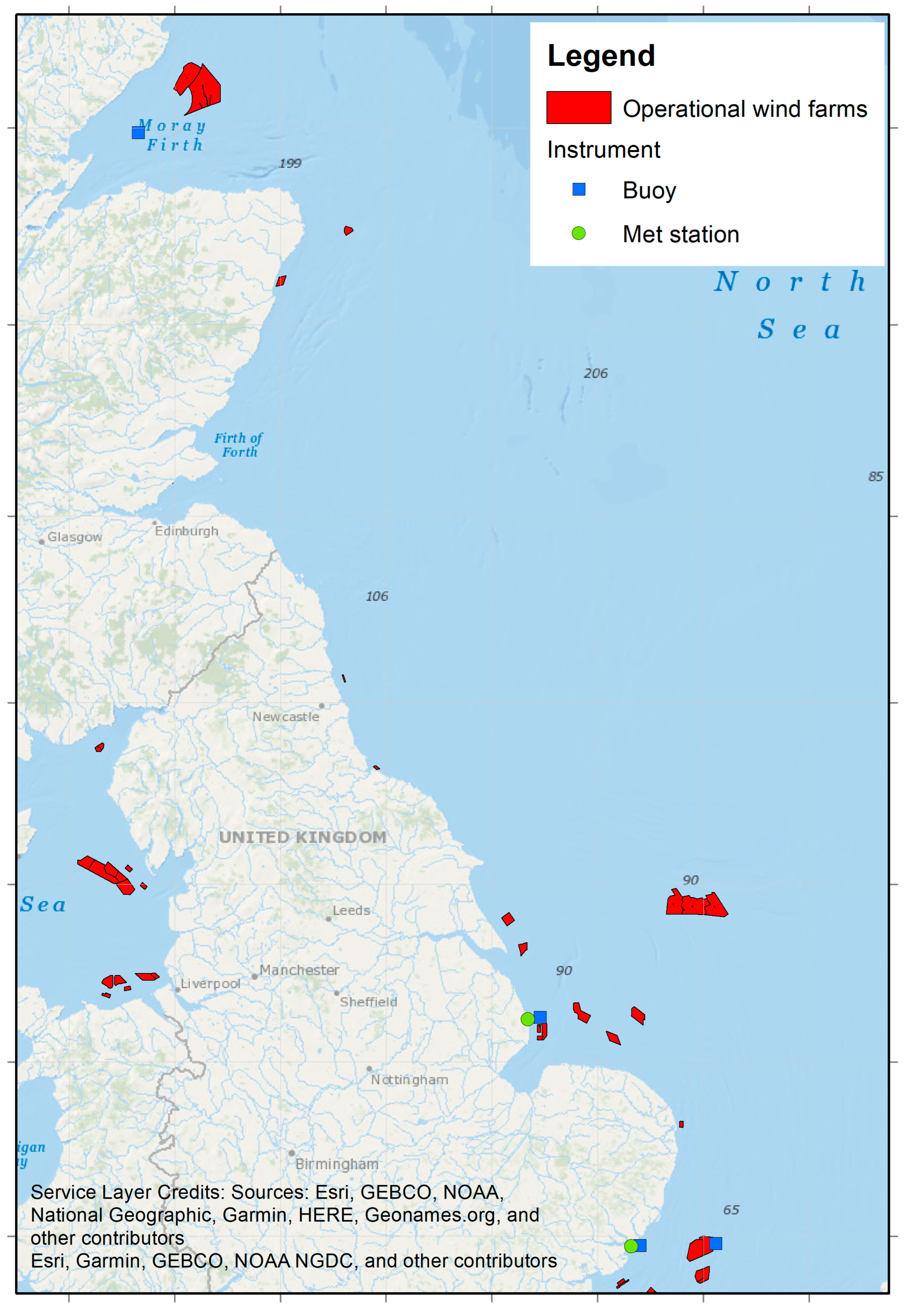
All products were expressed between January and October to match VMMS measurements and aggregated by mean to daily mean resolution in order to create daily dose values for technician welfare following the scope of the project.

2.3. Study Area

The study area covered latitudes between 51° N and 59° N in the North Sea. This was because VMMS data were collected from vessels deployed in four different wind farms in the North Sea which were operated by four different wind farm operators for spatial variability. The plot in Figure 1 presents a map of the North Sea area, showing operational offshore wind farms in the United Kingdom and the relevant available buoys and met stations considered in this project for metocean data validation. While the map shows operational wind farms in the region, the specific wind farms used to achieve the research aims are not highlighted, following the terms according to which the project data were made available.

2.4. Modelling the Welfare of Technicians

The objective of this research was to develop a dual-criterion welfare model that aids sailing decisions using proxy variables of the composite weighted RMS acceleration (aWRMS) and motion sickness incidence (MSI) to represent the levels of comfort and the likelihood of seasickness of technicians, respectively. Figure 2 presents the project workflow for achieving the research aim.
Our first target was to validate the metocean data and ensure that the sea-state data provided sufficient spatial coverage of transit routes travelled by participating CTVs. As such, data from buoys and met masts were used for validation and selected for their positions either in the path of the port of exit for participating CTVs or at the participating wind farms. The data from the in situ instruments were open source data provided by Cefas and funded by Environment Agency, licenced under the Cefas WaveNet Non-Commercial Licence v1.0, and from the channel coastal observatory (CCO) licenced under the Open Government Licence v3.0.
To explore human exposure to accelerations, the meteorological dataset, including variables of significant wave height, wave direction, wave period, sea surface height, current speed, current direction, wind speed, and wind direction, was merged into a dataset using dates as a merging variable in a MATLAB2018a workspace. An additional tidal range variable was created from the 15 min instantaneous resolution of the sea surface height variable in the current data rather than the daily mean to explore the impact of lunar tides on the proxy variables. This was achieved by finding the difference between the daily maximum and minimum sea surface height expressed in metres.
The proxy variables were developed from VMMS acceleration measurements. A variable for aWRMS was created from the expression in Equation (2) using the vector sum of accelerations including the x, y, and z axis, as well as the roll, pitch, and yaw accelerations following ISO 2631-1 guidance. The MSI variable was created from the expression in Equation (3) using the z-axis acceleration, also following ISO 2631-1 guidance. Applied weightings depend on the posture of passengers; as such, weightings in this study were applied under the assumption that technicians on the CTVs are in seated positions. As such, whole-body acceleration weighting for persons in seated positions was expressed as Wk for z-axis accelerations, Wd for x- and y-axis accelerations, We for rotational accelerations, and Wf for z-axis accelerations for MSI, including scaling factors of ‘kx = 1.4, ky = 1.4, kz = 1′ for the MSI and ‘kx = 1.0, ky = 1.0, kz = 1.0′ for aWRMS. The dataset of meteorological variables was then merged with the dataset of VMMS using join functions and dates as the key merging variables. Following this, a dimensionality reduction process was used to select a subset of the most relevant variables for the predictive modelling. This process was conducted to train models faster, simplify the models, improve accuracy, and reduce over-fitting where a model did not generalise well on unseen data based on the training data. As such, this process identified which input variables to include and which irrelevant variables to exclude for predictive modelling. This study used a filtering method to rank variables based on their correlation coefficient univariate metric [31], and principal component analysis (PCA) to identify the most relevant variables that make up most of the variance in predicting the proxy variables. These methods were chosen over the wrapper and embedding [32], which are embedded in the machine learning process and are not model-agnostic [33]. As such, domain knowledge could be applied to the dataset, such as the removal of redundant proxy variables such as the motion sickness dose value (MSDV), which also describes the likelihood of seasickness [34]. Seven variables were identified, accounting for 70% of the variation in predicting both proxy variables including vessel transit duration, vessel speed, vessel heading, significant wave height, current speed, current direction, and tidal height.
For the modelling process, the dataset of the identified variables was split into a training set of 637 transits (75% of the dataset) and a testing set of 212 transits (25%) using a hold-out function. This was performed following a standard machine learning approach to validate the performance of a model selected [35]. Therefore, the machine learning model was defined as the following general equation,
y ^ i = β 0 + i = 1 n β i X i + e i
where i = 1, 2… n; y ^ i is the proxy variable in the ith sample; Xi comprises the input variables in the ith sample; βi is the coefficient for the input variables and ei is the residual error.
The training set was trained against multiple regression models including linear regression models, regression trees, support vector machines, Gaussian process regression models, and ensemble trees. For each iteration, we assessed the model’s performance by calculating the coefficient of determination (R2) to account for the goodness of fit, and the mean squared error (MSE) and root mean squared error (RMSE) to provide a measure of how far apart model predictions were from estimated values. The machine learning process identified a Gaussian process regression (GPR) model as the model of best fit, which was tested on the testing set using a ‘ftrgp’ function to predict the proxy variables.
To deliver sailing decisions, we applied defined operational limits to the model’s predicting the proxy variables. Operational limits were defined by ISO 2631-1 for limits of human operation and limits of operation based on best seafaring practices. These included a limit equal to or greater than 0.32 ms−2 for predicted values of aWRMS discretised as progressively uncomfortable for technicians, and limits applied to the predictions of MSI equal to or greater than 20% discretised as unfavourable sailing conditions able to progressively induce seasickness in 20% or more of the population of technicians in transit. The resulting model was a binary decision support model that predicted sail and not-sail decisions from ‘if and else’ statements written in code in the MATLAB workspace.

3. Results and Discussion
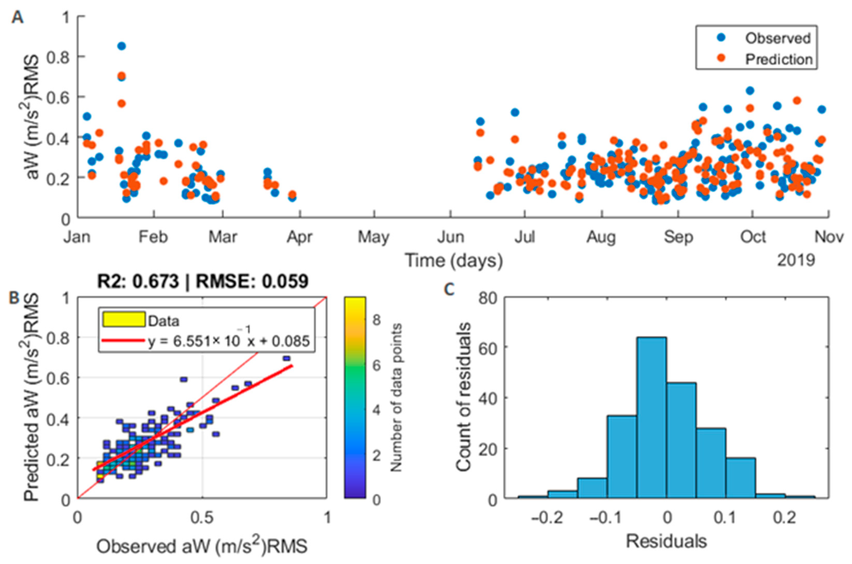
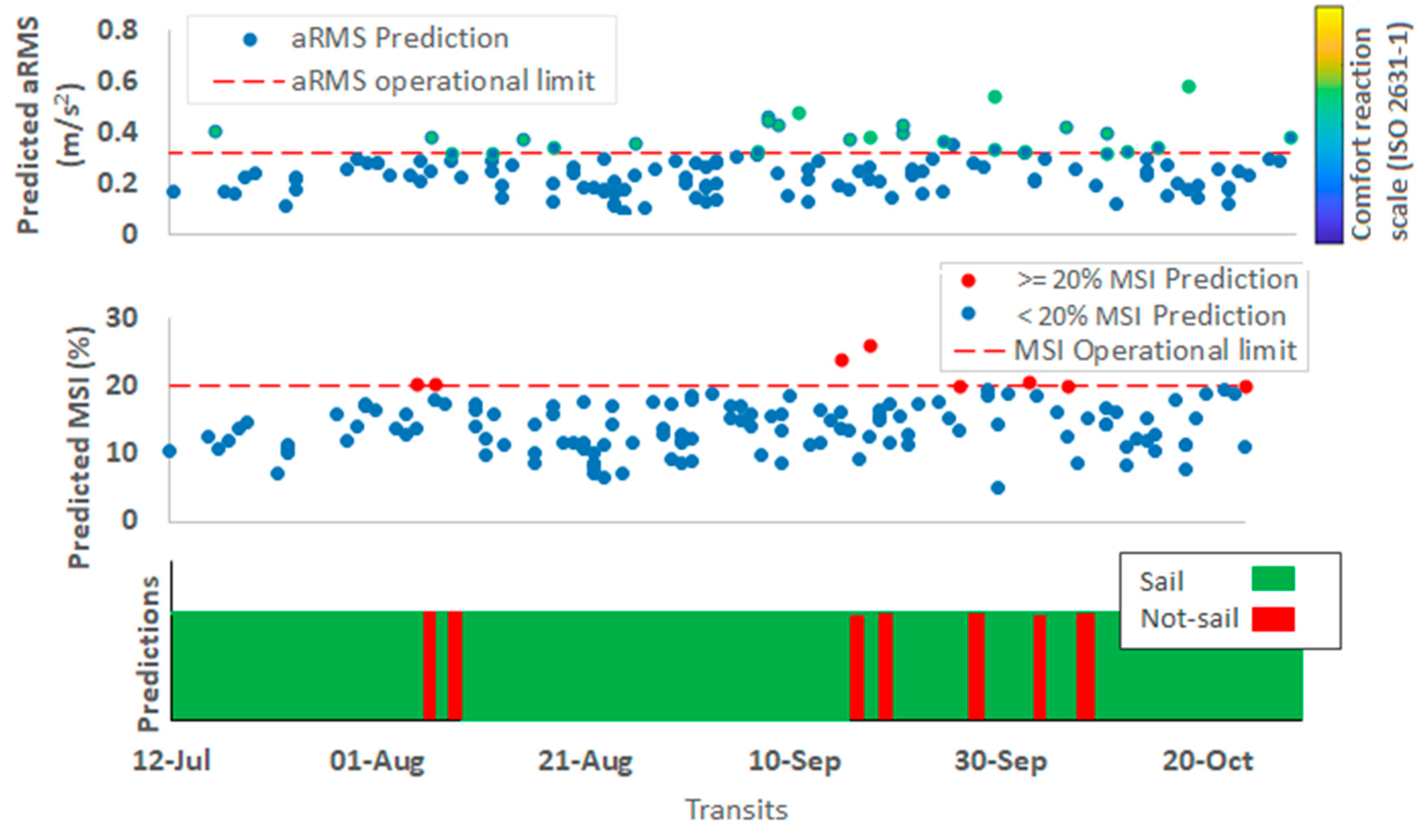
Our first step was to ensure the accurate description of transit routes in project sites and validate metocean data spatial coverage. Data from in situ devices such as buoys and data from met masts were compared with the metocean data at specific points during the transit of participating crew transfer vessels between ports and wind farms. The variables tested included significant wave height (m) and wind speed (ms−2). Table 2 below presents the results of the comparisons with available in situ devices.
The comparisons between metocean data and in situ data revealed good relationships between datasets, suggesting that metocean data products were able to provide accurate spatial coverage of the CTV routes when compared with available in situ data. Better relationships were found in the comparisons with significant wave height than with sea surface height and wind speed. This is likely due to the significant amount of missing data points in wind speed data.

Welfare Modelling

The process of dimension reduction revealed the most relevant variables to predict aWRMS and MSI, including vessel journey duration, vessel speed, tidal range, current speed, significant wave height, and current direction. Some identified variables are typically present in the parameters used when exploring comfort or the incidence of motion sickness, including journey duration due to the negative relationship between duration and magnitudes of acceleration [36,37], the relationship between vessel speed and magnitudes of acceleration [38], and significant wave height and MSI [34,39,40,41]. While other variables such as current speed, current direction, and tidal range are not typically present in parameters used in studies evaluating comfort and MSI, the dimensionality reduction process identified these parameters as relevant to the variance in predicting aWRMS and MSI. The identified variables were used as input variables to identify the model of best fit by training the training set against multiple regression models, shown in Table 3, which revealed a rational quadratic regression model.
The Gaussian process regression (GPR) model is a non-parametric method for machine learning regression which was used on a testing set. We show the results of the model generated using the MATLAB ‘ftrgp’ function with ‘KernelFunction = rationalquadratic’, ‘BasisFunction = constant’, ‘Standardize = true’, ‘PredictMethod = Exact’, as the model specification. The accuracy of the models was measured using their R2, MSE, and RMSE values, which are best used in measuring regression model performance [42]. These measures were chosen to identify how well the models predicted the proxy variables and present measures through which improved models can be tested against. Figure 3 and Figure 4 present the results of both models in predicting proxy variables.
Figure 3 and Figure 4 present model results for predicting the proxy variables. The response plot in (A) of both figures shows that predictions follow similar tracks to measured values. The plot of the correlation between predicted and measured aWRMS (Figure 3B) shows a moderate relationship between predicted and estimated values with an R2 value of 0.67. This shows that for this model, 67% of the variation of estimated aWRMS can be explained by the independent variables, and as such, only 33% reside in the residual. This provides a measure of improvements that need to be implemented in improving the model, which could include less significant measures such as increasing the size of the dataset to improve predictability and more significant measures such as unexplored or unknown factors that could influence the measured acceleration on the participating CTVs. The model’s errors are evaluated from RMSE values of 0.06 ms−2, and the histogram of residuals (Figure 3C) which shows that model predictions can be off by 0.25 ms−2; however, most data points are centred around zero, which suggests that the errors are not significant. Additionally, the presence of data points (the density plot in Figure 3B) above the perfect prediction line (thin red line) between 0.1 and 0.3 ms−2 and data points below the prediction line between 0.5 and 1.0 ms−2 shows that the model overestimated more common values of composite weighted acceleration and underestimates the less common values. Further statistical significance is presented by a p-value less than 0.05.
Similarly, Figure 4B presents a poor relationship between the predicted and estimated values of motion sickness incidence (MSI), with an R2 value of 0.49. This shows more than half of the variance, up to 51%, resides in the residual. As such, the variables explored do not make up most of the variation in predicting MSI. This shows that a significant amount of work needs to be done to improve the models’ prediction, and as such, the model does not present an acceptable level of performance. The RMSE values of 2.6% and the histogram of residuals in Figure 4C show that model predictions can be off by 2.6%; however, a p-value less than 0.05 shows that there is statistical significance. Table 4 presents the results of both models between training and testing sets.
It should be noted that the models do not predict comfort and seasickness in technicians, but rather the aWRMS and MSI as proxies for the levels of discomfort using the magnitude of aWRMS and the likelihood of seasickness using the percentage value of MSI. In addition, the comfort thresholds presented in the ISO 2631-1 are based on dated experimental studies [26] which might not be suitable for current assessments or suited to measurements on CTVs. Furthermore, MSI, as stated in Section 1, is the incidence of vomiting (a symptom of motion sickness) and does not account for other symptoms of motion sickness including sweating, changes in temperature, headaches [28], or other susceptibility factors associated with motion sickness such as temperature and a lack of visual reference [43]. This is highlighted in a recent publication by [43], who suggested improvements to the international standard to include more dimensions of motion sickness. As such, motion sickness incidence may not be a sufficient indicator of seasickness.
To predict sail and not-sail decisions, operational limits are applied to the model outputs of the aWRMS and MSI based on the operational limits defined by ISO 2631-1 for providing an approximate human comfort response to accelerations, and the best seafaring practices for limiting the incidence of motion sickness [5,8]. The limits applied include the categorisation of increasing values of RMS acceleration above 0.315 ms−2 as progressively uncomfortable and MSI values below 20% as limits of acceptable conditions. Therefore, the model created is based on a dual-criterion system established from magnitudes of predicted weighted acceleration and the predicted incidence of vomiting. Figure 5 presents the results of the technician welfare model with predicted sail and not sail decisions over three months.
Figure 5 presents 159 predictions based on the dual criterion operational limits applied to predictions of aWRMS and MSI. The coloured balls represent model predictions. For the aWRMS model, the balls range between blue and green showing levels of discomfort based on ISO 2631, and for the MSI model, the red balls indicate greater than or equal to 20% MSI values while the blue balls indicate less than 20% MSI. The final well-being model shows green, for sail, and red, for not-sail, bars which indicate sailing decisions derived from aWRMS and MSI model outputs. The welfare model predicted 129 sail decisions (shown in green) and 7 not-sail decisions (in red).

4. Conclusions

This research presents a holistic approach to an aspect of operations and maintenance planning typically not expressed in accounting for the welfare of technicians in transit by assessing comfort and the likelihood of seasickness. This can further inform their ability to perform work upon arrival at offshore turbines. Proxy indicators were used to describe comfort levels and the likelihood of seasickness in technicians, including aWRMS and MSI, respectively. These proxies used were selected due to their relationships with whole-body accelerations, which are supported by findings in the literature, including the relationship between the magnitude of RMS accelerations and levels of discomfort [6] and MSI as an indicator of the incidence of seasickness [5]. Significant contributions to the literature were made in describing the non-homogeneous random variables of sea-state and vessel operational parameters, as typically, studies on human exposure to acceleration calculate the RMS of vessel acceleration using a response amplitude operator (RAO) along with wave energy spectra to produce response spectra [42] or combine numerical ocean models to seat models, providing a range of sea state and vessel parameters for analysis [22]. This is because experimental in situ measurements of sea-state and vessel characteristics have limited spatial coverage and are time-consuming and expensive [22,44]. This research, however, benefits from measured vessel accelerations which allowed more variable exploration of parameters to identify relevant relationships for modelling.
The results of the models created present a framework for assessing welfare based on proxy variables; however, the performance of the models indicated that more work is needed to improve model predictability. In application, the welfare of technicians can be assessed before or alongside a maintenance transfer plan able to make sailing decisions that can account for the wellbeing of technicians. Therefore, this research can provide major contributions to the maintenance planning for offshore wind farms once the major limitations, outlined in Section 4.1, have been addressed. This is particularly important as typical CTV operational limits can make a wind farm accessible but perceived accelerations from transits may be unacceptable to technicians [7], potentially causing discomfort and seasickness [6] which can affect the ability to perform complex functions in technicians, including manual handling and cognitive tasks [18]. This research can also provide a framework for regulatory compliance, as the model-set acceleration limit falls below the limits set in the Control of Vibration at Work Regulations 2005 [45] which came into force in the UK in 2005, and the limits to MSI also aid wind farm operators with their duties of care to technicians under the Health and Safety at Work etc Act 1974 [46].

4.1. Limitations and Future Work

There are key limitations in this research that need to be addressed with areas where future work can be done.
The VMMS data used in this paper were collected for a different purpose than this project’s objectives and from a project with different objectives. The authors of this paper had limited control over the measurement of acceleration data, the positioning of the VMMS devices, and the calibration of the devices. In addition, there were restrictions on the data made available including the vessels used and subjective measurements, which prevented the validation of model results. For this reason, some assumptions had to be made within the course of this research regarding the calibration of the accelerometers in the VMMS and the placement of the VMMS on the participating vessels, which may have created errors due to the physical constraints of the device and the location of the device in relation to the personnel on board. The assumptions were made based on informal requests to the researchers within the original study, as well as the publication from the study [28]. In addition to this, the research objective had to be amended to the dataset available, which restricted the type of research questions generated for the project. Future research in this field will require a dataset designed for the research objectives to eliminate restrictions in data analysis and exploration, and reduce random errors.
The results of the model-predicted proxies could benefit from validations against real-life measurements of the comfort and seasickness of technicians in transit in the form of measured physiological changes or symptomatic questionnaires [43]. This would also inform the future exploration of input parameters and greatly improve the model. In addition to this, experimental studies cited in the international standard explored limits of operation for vessels of varying sizes, some of which are different from the CTVs used in O&M activities. As such, the operational limits can also be validated against measurements of comfort for CTVs.
Consideration also needs to be performed for the proxies used, including how discomfort is described and the definition of seasickness. While the relationship between RMS acceleration and the discomfort of passengers has been explored in the literature, the available literature is dated, and the nature of questionnaires used to assess discomfort and the type of vessels or simulations used can impact the ranges of discomfort experienced. Similarly, the model predicts the incidence of vomiting rather than the incidence of motion sickness and does not account for other relevant factors or other susceptibility factors associated with motion sickness [43]. For the technicians onboard CTVs completing complex work, the point of vomiting is well past the point where complex work can be performed, and as such, MSI may not be a useful benchmark for predicting wellbeing.
Future work also needs to be performed to iteratively improve model predictions by exploring more relevant variables for predicting aWRMS and MSI, including increasing the size of the dataset used in making predictions, applying other measurable welfare parameters not included in the welfare model, increasing the spatial variability to account for the sea-state characteristics of other regions, and improving vessel variability in predictions such as different sizes of CTVs, and other service vessels such as service operation vessels (SOVs) and daughter crafts.

Author Contributions

Conceptualisation, T.D.U.; methodology, T.D.U.; software, T.D.U.; resources, T.W.; data curation, T.D.U.; writing—original draft preparation, T.D.U.; writing—review and editing, R.F. and T.W.; visualisation, T.D.U.; supervision, R.F. and T.W. All authors have read and agreed to the published version of the manuscript.”

Funding

This research was supported by funding provided to the lead author by The University of Hull.

Data Availability Statement

Sea-state data for this study were obtained using Copernicus Marine Service products. Product information is presented below. Copernicus Marine Service Information, n.d. Atlantic- European Northwest Shelf- Wave Physics Reanalysis, NWSHELF_REANALYSIS_WAV_004_015. [Product] marine.copernicus.eu, https://doi.org/10.48670/moi-00060 [accessed on 20 January 2022]. Copernicus Marine Service Information, n.d. Atlantic—European Northwest Shelf—Ocean Physics Analysis and Forecast, NORTHWESTSHELF_ANALYSIS_FORECAST_PHY_004_013 [Product] marine.copernicus.eu, https://doi.org/10.48670/moi-00054 [accessed on 20 January 2022]. Copernicus Marine Service Information, n.d. Global Ocean Wind L4 Reprocessed 6 hourly Observations, WIND_GLO_WIND_L4_REP_OBSERVATIONS_012_006. [Product] marine.copernicus.eu, https://doi.org/10.48670/moi-00185 [accessed on 20 January 2022]. The authors elect to not share specific vessel data due to personal and commercial confidentiality.

Acknowledgments

This research was supported by funding to the first author from the University of Hull. The authors would like to thank BMO Offshore for providing access to VMMS.

Conflicts of Interest

The authors declare no conflict of interest.

References

  1. Scheu, M.; Matha, D.; Hofmann, M.; Muskulus, M. Maintenance strategies for large offshore wind farms. Energy Procedia 2012, 24, 281–288. [Google Scholar] [CrossRef] [Green Version]
  2. Ding, F.; Tian, Z. Opportunistic maintenance for wind farms considering multi-level imperfect maintenance thresholds. Renew Energy 2012, 45, 175–182. [Google Scholar] [CrossRef]
  3. Shafiee, M. Maintenance logistics organization for offshore wind energy: Current progress and future perspectives. Renew Energy 2015, 77, 182–193. [Google Scholar] [CrossRef]
  4. Seyr, H.; Muskulus, M. Decision Support Models for Operations and Maintenance for Offshore Wind Farms: A Review. Appl. Sci. 2019, 9, 278. [Google Scholar] [CrossRef] [Green Version]
  5. Phillips, S.; Shin, I.; Armstrong, C. Crew Transfer Vessel Performance Evaluation. In Design and Operation of Wind Farm Support Vessels: RINA International Conference; Phillips, S., Shin, I., Armstrong, C., Eds.; Royal Institution of Naval Architects: London, UK, 2015; pp. 1–5. Available online: https://app.knovel.com/web/toc.v/cid:kpDOWFSVR5/viewerType:toc/ (accessed on 23 November 2020).
  6. Mansfield, N.J. Human Response to Vibration 1; CRC Press: New York, NY, USA, 2005; Volume 1. [Google Scholar]
  7. Scheu, M.; Matha, D.; Schwarzkopf, M.A.; Kolios, A. Human exposure to motion during maintenance on floating offshore wind turbines. Ocean Eng. 2018, 165, 293–306. [Google Scholar] [CrossRef]
  8. Stevens, S.C.; Parsons, M.G. Effects of Motion at Sea on Crew Performance: A Survey. Mar. Technol. SNAME News 2002, 39, 29–47. [Google Scholar] [CrossRef]
  9. Griffin, M.J. Handbook of Human Vibration, 1st ed.; Academic Press Limited: London, UK, 1990; Volume 1. [Google Scholar]
  10. Cardinale, M.; Pope, M.H. The effects of whole body vibration on humans: Dangerous or advantageous? Acta Physiol. Hung. 2003, 90, 195–206. [Google Scholar] [CrossRef]
  11. Coyte, J.L.; Stirling, D.; Du, H.; Ros, M. Seated Whole-Body Vibration Analysis, Technologies, and Modeling: A Survey. IEEE Trans. Syst. Man. Cybern. Syst. 2016, 46, 725–739. [Google Scholar] [CrossRef]
  12. Mette, J.; Garrido, M.V.; Harth, V.; Preisser, A.M.; Mache, S. Healthy offshore workforce? A qualitative study on offshore wind employees’ occupational strain, health, and coping. BMC Public Health 2018, 18, 172. [Google Scholar] [CrossRef] [Green Version]
  13. Reason, J.T.; Brand, J.J. Motion Sickness, 1st ed.; Academic Press Inc.: London, UK, 1975; Volume 1. [Google Scholar]
  14. O’Hanlon, J.F.; McCauley, M.E. Motion sickness incidence as a function of the frequency and acceleration of vertical sinusoidal motion. Aerosp. Med. 1974, 45, 366–369. [Google Scholar] [CrossRef] [Green Version]
  15. Donohew, B.E.; Griffin, M.J. Motion sickness: Effect of the frequency of lateral oscillation. Aviat. Space Environ. Med. 2004, 75, 649–656. [Google Scholar] [PubMed]
  16. Wertheim, A.H.; Bos, J.E.; Bles, W. Contributions of roll and pitch to sea sickness. Brain Res. Bull. 1998, 47, 517–524. [Google Scholar] [CrossRef] [PubMed]
  17. Dobie, T.G. Motion Sickness: A Motion Adaptation Syndrome; Springer: New Orleans, LA, USA, 2019; Volume 6. [Google Scholar]
  18. Matsangas, P.; McCauley, M.E.; Becker, W. The effect of mild motion sickness and sopite syndrome on multitasking cognitive performance. Hum. Factors 2014, 56, 1124–1135. [Google Scholar] [CrossRef] [PubMed]
  19. Zhang, L.L.; Wang, J.Q.; Qi, R.R.; Pan, L.L.; Li, M.; Cai, Y.L. Motion Sickness: Current Knowledge and Recent Advance. CNS Neurosci. Ther. 2016, 22, 15–24. [Google Scholar] [CrossRef]
  20. Marjanen, Y.; Mansfield, N.J. Application of ISO 2631-1 (1997) for evaluating discomfort from whole-body vibration: Verification using field and laboratory studies. In Proceedings of the 40th International Congress and Exposition on Noise Control Engineering 2011, INTER-NOISE, Osaka, Japan, 4–7 September 2011; pp. 3475–3480. [Google Scholar]
  21. Newell, G.S.; Mansfield, N.J. Evaluation of reaction time performance and subjective workload during whole-body vibration exposure while seated in upright and twisted postures with and without armrests. Int. J. Ind. Ergon. 2008, 38, 499–508. [Google Scholar] [CrossRef]
  22. Olausson, K. On Evaluation and Modelling of Human Exposure to Vibration and Shock on Planing High-Speed Craft. Licentiate Thesis, KTH Royal Institute of Technology: Stockholm, Sweden, 2015. [Google Scholar]
  23. Leung, A.W.S.; Chan, C.C.H.; Ng, J.J.M.; Wong, P.C.C. Factors contributing to officers’ fatigue in high-speed maritime craft operations. Appl. Ergon. 2006, 37, 565–576. [Google Scholar] [CrossRef] [Green Version]
  24. ISO 2631-1; Mechanical Vibration and Shock-Evaluation of Human Exposure to Whole-Body Vibration. International Organization for Standardization: Geneva, Switzerland, 1997.
  25. Huston, D.R.; Zhao, X.; Johnson, C.C. Whole-body shock and vibration: Frequency and amplitude dependence of comfort. J. Sound Vib. 2000, 230, 964–970. [Google Scholar] [CrossRef]
  26. Shoenberger, R.W. Discomfort judgements of translational and angular whole-body vibrations. Aviat. Space Environ. Med. 1982, 53, 454–457. Available online: https://pubmed.ncbi.nlm.nih.gov/7092753/ (accessed on 14 June 2022).
  27. Offshore Energy. BMO Offshore Presents CTV Engine Monitoring—Offshore Energy. Offshore-energy.biz. 19 July 2016. Available online: https://www.offshore-energy.biz/bmo-offshore-presents-ctv-engine-monitoring/ (accessed on 3 November 2022).
  28. Earle, F.; Huddlestone, J.; Williams, T.; Stock-Williams, C.; van der Mijle-Meijer, H.; de Vries, L.; van Heemst, H.; Hoogerwerf, E.; Koomen, L.; de Ridder, E.-J.; et al. SPOWTT: Improving the safety and productivity of offshore wind technician transit. Wind Energy 2021, 25, 34–51. [Google Scholar] [CrossRef]
  29. Lewis, H.W.; Sanchez, J.M.C.; Siddorn, J.; King, R.R.; Tonani, M.; Saulter, A.; Sykes, P.; Pequignet, A.-C.; Weedon, G.P.; Palmer, T.; et al. Can wave coupling improve operational regional ocean forecasts for the north-west European Shelf? Ocean Sci. 2019, 15, 669–690. [Google Scholar] [CrossRef] [Green Version]
  30. Tonani, M.; Sykes, P.; King, R.R.; McConnell, N.; Péquignet, A.-C.; O’Dea, E.; Graham, J.A.; Polton, J.; Siddorn, J. The impact of a new high-resolution ocean model on the Met Office North-West European Shelf forecasting system. Ocean Sci. 2019, 15, 1133–1158. [Google Scholar] [CrossRef] [Green Version]
  31. Kumari, B.; Swarnkar, T. Filter versus Wrapper Feature Subset Selection in Large Dimensionality Micro array: A Review. Int. J. Comput. Sci. Inf. Technol. 2011, 2, 1048–1053. [Google Scholar]
  32. Chandrashekar, G.; Sahin, F. A survey on feature selection methods. Comput. Electr. Eng. 2014, 40, 16–28. [Google Scholar] [CrossRef]
  33. Lal, T.N.; Chapelle, O.; Western, J.; Elisseeff, A. Embedded methods. In Feature Extraction. Studies in Fuzziness and Soft Computing; Springer: Berlin/Heidelberg, Germany, 2006; pp. 137–165. [Google Scholar] [CrossRef]
  34. Cepowski, T. The prediction of the Motion Sickness Incidence index at the initial design stage. Zesz. Nauk. Akad. Morska W Szczec. 2012, 31, 45–48. [Google Scholar]
  35. Stetco, A.; Dinmohammadi, F.; Zhao, X.; Robu, U.; Flynn, D.; Barnes, M.; Keane, J.; Nenadic, C. Machine learning methods for wind turbine condition monitoring: A review. Renew Energy 2019, 133, 620–635. [Google Scholar] [CrossRef]
  36. Griffin, M.J.; Whitham, E.M. Time dependency of whole-body vibration discomfort. J. Acoust. Soc. Am. 1998, 68, 1523. [Google Scholar] [CrossRef]
  37. Maeda, S.; Morioka, M. Measurement of whole-body vibration exposure from garbage trucks. J. Sound Vib. 1998, 215, 959–964. Available online: https://www.academia.edu/8126588/MEASUREMENT_OF_WHOLE_BODY_VIBRATION_EXPOSURE_FROM_GARBAGE_TRUCKS (accessed on 9 January 2022). [CrossRef]
  38. Eger, T.; Contratto, M.; Dickey, J. Influence of Driving Speed, Terrain, Seat Performance and Ride Control on Predicted Health Risk Based on ISO 263I-I and EU Directive 2002/44/EC:. J. Low Freq. Noise Vib. Act. Control 2011, 30, 291–312. [Google Scholar] [CrossRef] [Green Version]
  39. Cepowski, T. On the modeling of car passenger ferryship design parameters with respect to selected sea-keeping qualities and additional resistance in waves. Pol. Marit. Res. 2009, 16, 3–10. [Google Scholar] [CrossRef] [Green Version]
  40. Rumawas, V.; Asbjørnslett, B.E.; Klöckner, C.A. Human Factors Evaluation in Ship Design and Operation: An Case Study in Norwegian Sea. In Maritime Safety International Conference (MASTIC 2018); CSP: Bali, Indonesia, 2018; pp. 66–78. [Google Scholar]
  41. Piscopo, V.; Scamardella, A. The overall motion sickness incidence applied to catamarans. Int. J. Nav. Archit. Ocean Eng. 2015, 7, 655–669. [Google Scholar] [CrossRef]
  42. Jenkins, B.; Prothero, A.; Collu, M.; Carroll, J.; McMillan, D.; McDonald, A. Limiting Wave Conditions for the Safe Maintenance of Floating Wind Turbines. J. Phys. Conf. Ser. 2021, 2018, 012023. [Google Scholar] [CrossRef]
  43. Bos, J.E.; Diels, C.; Souman, J.L.; Rahmatalla, S.; Boileau, P.-É. Beyond Seasickness: A Motivated Call for a New Motion Sickness Standard across Motion Environments. Vibration 2022, 5, 755–769. [Google Scholar] [CrossRef]
  44. Medina-Lopez, E.; McMillan, D.; Lazic, J.; Hart, E.; Zen, S.; Angeloudis, A.; Bannon, E.; Browell, J.; Dorling, S.; Dorrell, R.; et al. Satellite data for the offshore renewable energy sector: Synergies and innovation opportunities. Remote Remote Sens. Environ. 2021, 264, 112–588. [Google Scholar] [CrossRef]
  45. UK Government. The Control of Vibration at Work Regulations 2005; UK Statutory Instruments: London, UK, 2005. Available online: https://legislation.gov.uk (accessed on 16 March 2022).
  46. UK Government. Health and Safety at Work etc Act; UK Statutory Instruments: London, UK, 1974; pp. 1–166. Available online: https://legislation.gov.uk (accessed on 16 March 2022).
Figure 1. Locations of available operational wind farms in red-coloured polygons, with relevant buoys in blue, and met stations in green. The image contains data provided by The Crown Estate that are protected by copyright and database rights, Cefas, licensed under the Cefas WaveNet Non-Commercial Licence v1.0, and the channel coastal observatory (CCO), licenced under the Open Government Licence v3.0.
Vibration 06 00027 g001
Figure 2. Project workflow for assessing the welfare of technicians in transit.
Vibration 06 00027 g002
Figure 3. Plots showing the model performance. (A) A response plot showing observed (measured), in blue, and predicted composite weighted RMS acceleration (aWRMS), in orange, with time. (B) The correlation between predicted and observed aWRMS (m/s2) showing the density of data points. (C) A histogram of residuals.
Vibration 06 00027 g003
Figure 4. Plots showing the model performance. (A) A response plot showing observed (measured), blue, and predicted motion sickness incidence (MSI), orange, with time. (B) The correlation between predicted and observed MSI (%) with a density of data points. (C) A histogram of residuals.
Vibration 06 00027 g004
Figure 5. A plot of the technician welfare model showing sail and not-sail decisions based on applied operational limits.
Vibration 06 00027 g005
Table 1. Estimations of comfort response to vibrations (ISO 2631-1, 1997).
The Magnitude of Acceleration in ms−2Comfort Reaction
Less than 0.315Not uncomfortable
0.315–0.63A little uncomfortable
0.5–1Fairly uncomfortable
0.8–1.6Uncomfortable
1.25–2.5Very uncomfortable
Greater than 2Extremely uncomfortable
Table 2. Comparisons between metocean data and in situ measurements showing statistical relevance.
CategoryR2RMSEp-ValueLocations
Significant wave height0.890.20<0.05Project site 1
Significant wave height0.840.25<0.05Project site 3
Significant wave height0.860.15<0.05Project site 4
Wind speed0.541.74<0.05Project site 1
Wind speed0.8470.213<0.05Project site 4
Table 3. Summary of trained models used to identify the model of best fit.
Regression ModelR2 (aWRMS)RMSE (aWRMS)R2 (MSI)RMSE (MSI)
Linear0.510.080.294.63
Interactions linear0.520.080.274.68
Robust linear0.500.090.284.64
Stepwise linear0.530.080.274.69
Fine tree0.400.090.254.77
Medium tree0.430.090.304.62
Coarse tree0.460.090.314.57
Linear SVM0.500.090.274.68
Quadratic SVM0.540.080.374.35
Cubic SVM0.540.080.384.32
Fine Gaussian SVM0.210.120.244.78
Medium Gaussian SVM0.560.080.414.20
Coarse Gaussian SVM0.510.080.334.47
Boosted tree0.580.080.454.02
Bagged trees0.560.080.454.02
Squared exponential GPR0.610.080.434.02
Matern 5/2 GPR0.590.080.424.02
Exponential GPR0.600.080.434.02
Rational quadratic GPR0.630.070.464.02
Table 4. Summary of model results for training and testing datasets.
RMSE R2MSESpeed (s)Time (s)Model
Training set0.070.630.00525,00012.11aWRMS Rational quadratic GPR (ms−2)
Testing set0.060.670.00488003.05
Training set4.020.4616.1524,00016.56MSI Rational quadratic GPR (%)
Testing set2.640.496.97880012.11
Disclaimer/Publisher’s Note: The statements, opinions and data contained in all publications are solely those of the individual author(s) and contributor(s) and not of MDPI and/or the editor(s). MDPI and/or the editor(s) disclaim responsibility for any injury to people or property resulting from any ideas, methods, instructions or products referred to in the content.

