Unsteady Aerodynamic Lift Force on a Pitching Wing: Experimental Measurement and Data Processing

Abstract

This work discusses the experimental challenges and processing of unsteady experiments for a pitching wing in the low-speed wind tunnel of the Vrije Universiteit Brussel. The setup used for unsteady experiments consisted of two independent devices: (a) a position control device to steer the pitch angle of the wing, and (b) a pressure measurement device to measure the aerodynamic loads. The position control setup can pitch the wing for a range of frequencies, amplitude, and offset levels. In this work, a NACA-0018 wing profile was used with an aspect ratio of 1.8. The position control and the pressure measurement setups operate independently of each other, necessitating advanced signal processing techniques to synchronize the pitch angle and the lift force. Furthermore, there is a (not well-documented) issue with the (sampling) clock frequency of the pressure measurement setup, which was resolved using a fully automated spectral analysis technique. The wing was pitched using a simple harmonic sine excitation signal at eight different offset levels (between 6° and 21°) for a fixed amplitude variation (std) of 6°. At each offset level, the wing was pitched at five different frequencies between 0.1 Hz and 2 Hz (that correspond to reduced frequencies k ranging from 0.006 to 0.125). All the experiments were conducted at a fixed chord-based Reynolds number of 2.85 × 10⁵. The choice of operating parameters invokes the linear and nonlinear behavior of the wing. The linear unsteady measurements agreed with the analytical results. The unsteady pressure measurements at higher offset levels revealed the nonlinear aerodynamic phenomenon of dynamic stall. This confirms that a nonlinear and dynamic model is required to capture the salient characteristics of the lift force on a pitching wing.

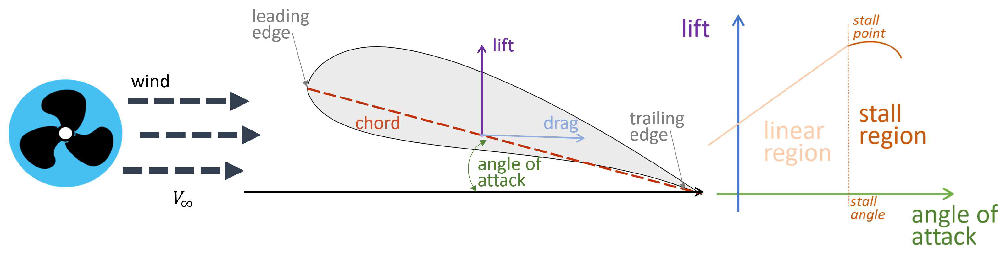
1. Introduction

The study of pitching wings is crucial for the design and development of rotary and flapping wing configurations [1,2,3]. Recent interest in the development of small-scale unmanned aerial vehicles (UAVs) and micro aerial vehicles (MAVs) is sparking an increasing interest in the unsteady aerodynamics of low aspect ratio (AR) wings at low Reynolds numbers [4] and in the construction of reduced-order models thereof [5,6,7]. The aerodynamic forces on the pitching wing in air at low altitude depend upon a range of geometrical (wing profile, aspect ratio, pitch angle, etc.) and flow parameters such as the Reynolds number and the turbulence intensity level [8,9,10]. Thus, a versatile experimental setup is required to reproduce the relevant unsteady flow conditions such as the active aeroelastic test bench setup developed in [11,12]. This setup was modified in this work to conduct pitching-wing experiments at high pitch angles to measure the unsteady surface pressure distribution and capture dynamic stall. The aerodynamic terminologies used in this work are illustrated in the conceptual drawing in Figure 1. The experimental setup consisted of a wing position control mechanism and the wing pressure measurement setup was installed in the low-speed wind tunnel (see Figure 2, Figure 3 and Figure 4) of the Vrije Universiteit Brussel. The setup allowed us to impose any arbitrary motion (within the bandwidth of the system). However, we focused on simple harmonic motions in this work.

When considering the lift force on a pitching wing as an “output signal” produced by a causal “dynamic system” as a response to a varying angle of attack, the “input” signal, the modeling, and analysis of the pitching wing can be approached as a typical vibro-acoustic problem. The lift force will be a linear or nonlinear (dynamic) function of the angle of attack, depending on the reduced frequency and the pitch angle [13] (for computational details see Section 3.4). At higher pitch angles, the lift force exhibits nonlinear phenomena such as higher harmonics and bifurcations [14,15]. These nonlinearities are mainly triggered by the interaction of the boundary layer and the dynamic stall vortex (DSV) [16,17]. A number of experimental [18,19,20,21,22] and numerical studies [23,24,25,26,27] have addressed the effect of the DSV on the lift distribution of wings. Most of these studies were for a wing aspect ratio of more than 3. In the case of low aspect ratio (LAR) wings, which are generally defined as an aspect ratio below 3 [28], the lift force is strongly dominated by the tip vortices and their interaction with the DSV [4,19,26]. In addition, there is a limited number of studies for LAR wings with conventional (non-flat-plate) wing profiles [4] such as the NACA-0018 used in this work. Such profiles could be more interesting for use in UAVs and MAVs [29,30].

In this work, we aimed (1) to describe the experimental setup and the use of advanced signal processing tools to deal with practical challenges related to unsteady aerodynamic experiments, and (2) to present the unsteady dynamic lift forces on a pitching LAR wing from a vibro-acoustic perspective. In particular, we identified the linear and nonlinear responses of the pitching wing and showed that any model of these unsteady loads should be nonlinear and dynamic.

The rest of this article is structured as follows. The experimental setup is described in Section 2. The details of the pitch control setup (Section 2.2) and the pressure measurement setup (Section 2.3) are important to understand the data-post processing explained in Section 3. Quasi-steady experiments are shown in Section 4, which highlight the linear and nonlinear regions of the pitching wing. The unsteady pitching wing experiments for a range of frequencies and offset levels are discussed in Section 5, with conclusions drawn in Section 6.

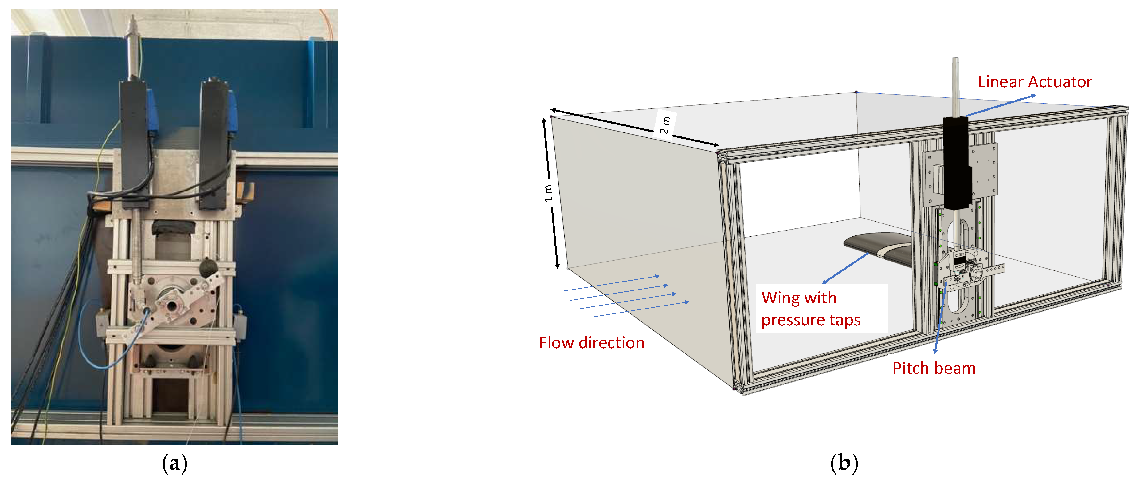
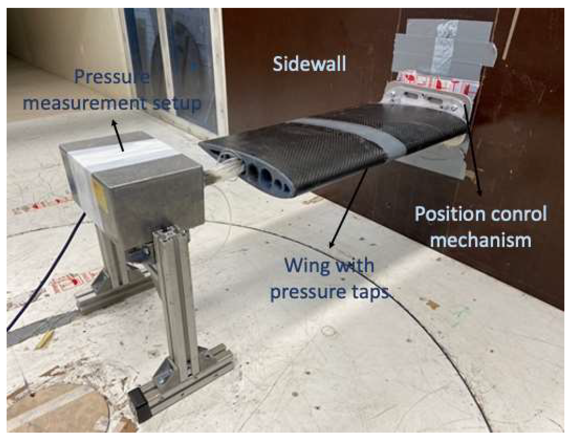
2. Experimental Setup

In this section, we describe the experimental setup that was used to acquire the lift forces on the pitching wing. From the perspective of an input–output system block, the pitch angle α can be considered as the input, and the lift force coefficient cl is the output of the system. The input and the output were generated and measured with two separate setups in the wind tunnel. The details of the wind tunnel are given in Section 2.1 and the α (pitch angle) control, which was attached to the wind tunnel sidewall, are elaborated in Section 2.2. The lift force coefficient cl is calculated from the pressure measurements on the wing. The pressure is obtained from pressure taps on the wing, which are connected to the pressure measurement system (further elaborated in Section 2.3).

2.1. Wind Tunnel

All experiments were conducted in the large low-speed open-circuit wind tunnel of the Vrije Universiteit Brussel. The test section has dimensions of 2000 mm × 1000 mm and an overall length of 12 m. The wind tunnel can operate at a maximum wind speed of 20 m/s. The wind velocity was measured using a pitot-static tube located upstream of the test section. The turbulence intensity of the freestream was less than 0.5% for all of the speeds at which the experiments were conducted.

The wing was a NACA–0018 with a 300 mm chord length and a span of 540 mm. The chord-based Reynolds number used in this study was 285 × 103, which corresponded to a freestream velocity of 15 m/s. The boundary layer at this Reynolds number and level of turbulence intensity will transition from laminar to turbulent over the wing surface. Small vertical-axis wind turbines and UAVs typically operate in this range. The freestream turbulence has a significant effect on the aerodynamic forces on the wing [31]. For the sake of simplicity, in this study, we limited the analysis to a single Reynolds number and turbulence intensity level.

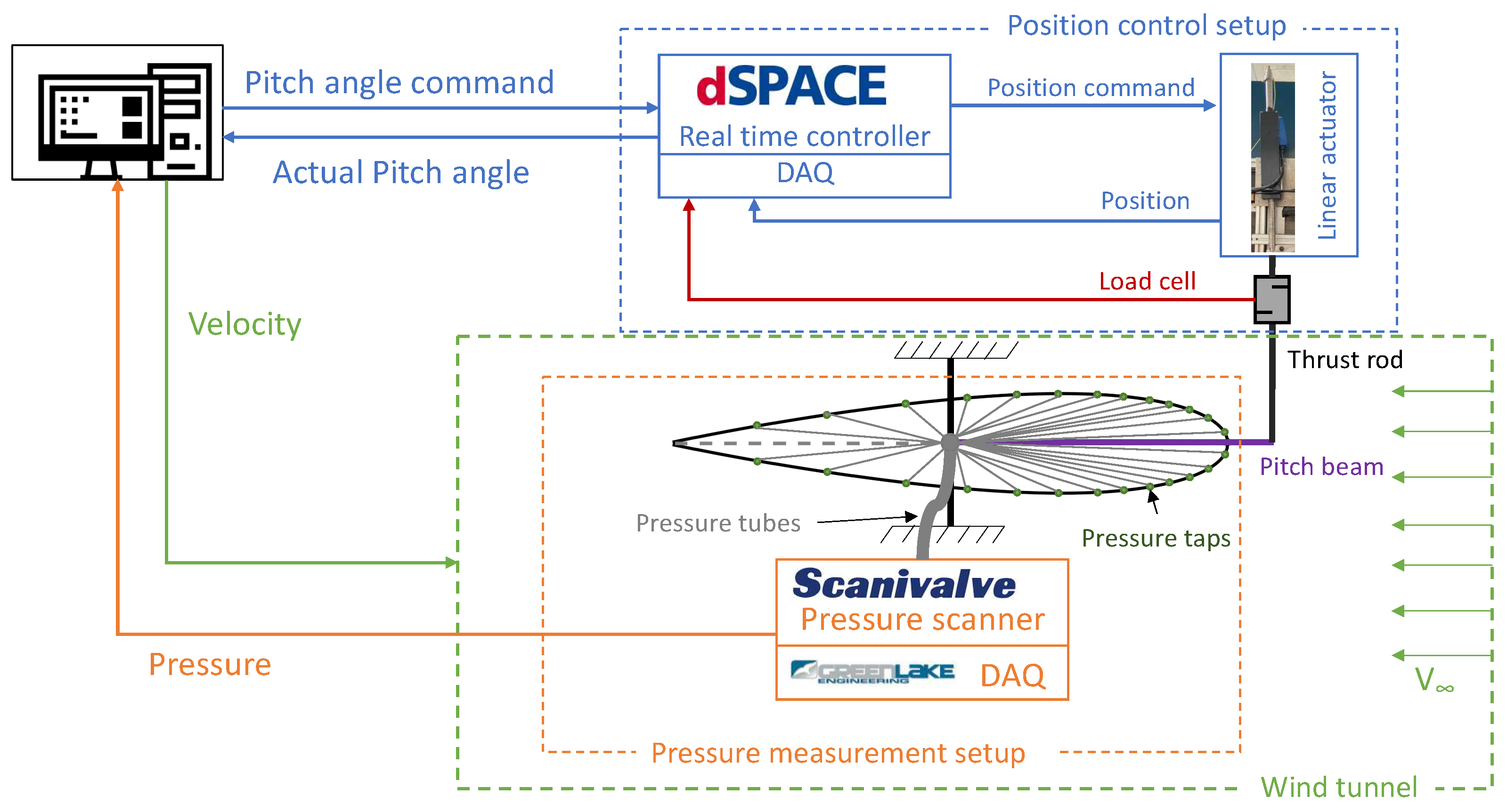
2.2. Position Control Setup

The position control mechanism can arbitrarily move the wing with a frequency band up to 5 Hz and pitch amplitudes up to a 30 degree pitch angle. In this study, we only used simple harmonic pitching. The pitching motion was achieved by the movement of a linear actuator connected with the wing using a pitch beam, as shown in Figure 2. The pitch mechanism was designed as a closed kinematic loop. Thus, the position of the wing was completely defined by the position of the actuator rod. Since the movement of the actuator rod is measured continuously, the position of the wing is also known at every time instant.

At the heart of the position control setup is a dSPACE^® ds-1103 real-time controller that imposes the motion of the actuator and hence the wing. The dSPACE^® controller has a PC-based controller card that is programmed using SIMULINK^® block diagrams that are downloaded into the memory of the controller. The SIMULINK^® program is then executed on the controller, and communication with the PC is only used to update the controller parameters or for data acquisition purposes. Thus, the dSPACE^® controller offers an interactive and flexible platform for actuator control. To ensure a precise position control, the dSPACE^® was run at 2 kHz. The data captured by the controller were logged at a 200 Hz sampling frequency ($f_s$). The choice of 200 Hz was due to the limitation of the pressure measurement setup, as will be explained in Section 3.3.

Figure 2. Schematic representation of the position control mechanism attached to the wind tunnel. (a) Actual view; (b) CAD model.

Figure 2. Schematic representation of the position control mechanism attached to the wind tunnel. (a) Actual view; (b) CAD model.

The desired pitch command was coded in SIMULINK^® and loaded in dSPACE^® memory. The controller converts the pitch command into a position command for the linear actuator. The linear actuator was fitted with a digital encoder that provided the actual position of the linear actuator with an accuracy of 0.0125 mm. This position was then translated into the pitch angle and sent back to the PC. A classical PID control algorithm was used in dSPACE^® for the pitch angle control [32]. The schematic of the experimental setup with the details of the position control setup is shown in Figure 4.

2.3. Pressure Measurement Setup

The pressure measurement setup consisted of the wing with pressure taps connected to a pressure scanner system via urethane tubes, as shown in Figure 3. The wing was made in three sections: two outer carbon fiber sections and a 3D-printed section in the middle. The 3D-printed section had 48 taps with the diameter of 0.8 mm. Each of the pressure taps was connected to the pressure scanner using a urethane tube with a length of 400 mm. All the tubing used in the experiments were of the same length. Using the analytical techniques described in [33], we found that the maximum amplification in the pressure signal for the maximum frequencies applied in our work was 0.03% and the phase lag was −0.3°, which we considered negligible for our purpose.

Figure 3. Pressure measurement setup connected to the rubber tubes attached to the wing taps.

Figure 3. Pressure measurement setup connected to the rubber tubes attached to the wing taps.

The schematic of the pressure measurement setup is shown in Figure 4. The pressure scanner used was a ZOC33/64Px Scanivalve measurement system that can measure the 64 channels simultaneously. A miniaturized data acquisition unit GLE/SmartZOC-100 from Greenlake Engineering was used, which is specifically designed to be interfaced with the Scanivalve ZOC pressure scanner systems. The unit provides the regulated and isolated voltage supply to the Scanivalve ZOC module, controls the scanning sequence, the conditioning for the analogue pressure transducers, and the 16-bit A/D conversion of the signals. The acquired data can be stored on a PC via an Ethernet bus connection. The specifications for the data acquisition (DAQ) system are given in

Table 1. The GLE/SmartZOC-100 specifications.

System accuracy	0.08 % FS or better, accordingly to the used pressure scanner
A/D resolution	16 bit
Scan rate	Ethernet data transfer: up to 500 S/ch/s with 64 ch ZOC

. The DAQ system gave an offset in the sampling frequency settings, which is discussed in Section 3.3.

Figure 4. Schematic of the experimental setup with a detailed description of the position control and pressure measurement setup.

Figure 4. Schematic of the experimental setup with a detailed description of the position control and pressure measurement setup.

3. Post-Processing of the Experimental Data

This section describes the different post-processing steps performed on the experimental data. This included a step to ensure that the input and output data were synchronized and had the same sampling frequency. Any bias in the pitch angle due to geometric uncertainties/initial offset in the wing was also removed.

3.1. Synchronization of the Input and Output Data

The dSPACE drive system, which controls the input (pitch angle α) signal, and the GLE/SmartZOC, which records the output (pressure), were not connected to a single interface. Initial attempts to integrate the pressure scanner system with the dSPACE^® controller failed since the GLE/SmartZOC data acquisition system is a proprietary device, prohibiting such an interface. A second attempt to directly integrate the Scanivalve^® to the same PC that was running the dSPACE program also failed. A programmable LabVIEW-steered DAQ similar to the GLE/SmartZOC hardware proved unable to achieve the desired sampling frequency. Additionally, the use of a trigger signal to synchronously start the pressure scanner system with the wing pitching was prohibited by the GLE/SmartZOC. Finally, we decided to synchronize in the post-processing step.

From a theoretical point of view, the proper synchronization of the two datasets is essential as it may result in falsely interpreting the distortions as frequency leakage/time variations (skirt-like shapes in the spectrum) or a false type of nonlinearity at a high level (where phases of input-output data play an important role) [34,35,36,37]. Our first tries involved linear cross-correlation of the input and the output signal to determine the starting position. However, this technique cannot be used reliably at a high angle of attacks near the stall region because the relationship between the input and output is nonlinear.

This led us to design a so-called starting signal, which was added at the start of every measurement. The starting signal consisted of three periods (pitch cycles) of a simple harmonic sine at a low frequency of 0.2 Hz (k = 0.013) with an amplitude of 5° at zero offset. The lift response of the wing at these pitch conditions was expected (and later demonstrated, see Section 4) to be linear. Therefore, a linear cross-correlation technique could be used reliably. The lag was estimated using the Fourier transform of the two datasets: the difference between the angles of the Fourier transform of the two signals corresponded to the phase shift (delay). Once the delay is estimated, the two signals can be properly resynchronized. Figure 5 shows the original output signal and the corrected output signal after synchronization with the input data. The accuracy of the method is ≤±1/$f_s$, which is ≤±5 ms for the sampling frequency used in this work. This method can, in principle, be generalized to broadband signals such as multisines or swept-sines in the future.

3.2. Angle of Attack Correction

As mentioned earlier in Section 2.1, the kinematics of the pitching mechanism is closed-loop, and the movement of the actuator can be used precisely to calculate the exact pitch angle. It is important to explain here that the linear actuator rod fully relaxes when powered off. At the controller start up, the user has to provide the exact pitch angle, which the controller takes as the reference. Thus, each time during controller power up, the wing was brought to a zero-pitch angle manually. This was achieved by using a digital inclinometer with an accuracy of ±0.1°. The inclinometer was first calibrated by placing it on the wind tunnel floor, thus the zero-pitch angle was taken with reference to the wind tunnel floor.

To cater for slight misalignment or manufacturing inaccuracies in the wing profile design, the angle of attack can be further corrected in the post-processing step. This was conducted by using the starting signal (i.e., single sine at 0.2 Hz with maximum pitch amplitude of 5°). Since the relationship between the lift and the pitch angle is linear in this operating regime, a linear fit was carried out between the lift coefficient and the angle of attack. The intercept of the linear fit gives the zero error in the angle of attack. The intercept is then added to the angle of attack measurement to correct for any pitch angle misalignment.

3.3. Sampling Frequency Correction of the Pressure Signal

The data acquisition system used for the pressure scanner (the GLE/SmartZOC) provides several possibilities for the sampling frequency, depending on the number of active channels. Since we used 64 channels, the device has a limitation to log the data at the maximum of 500 Hz. However, the initial experiments at 500 Hz were plagued by issues that were not evident in shorter and lower-frequency measurements. Experiments of more than 250 s at a simple harmonic sine of 2 Hz (e.g., showed a constantly increasing lag between the angle of attack and the lift force), as shown in Figure 6a. This kind of undesired behavior is problematic due to two interrelated reasons. The output signal (lift force) would lag more and more and eventually start to lead the (periodic sinusoidal) input signal (angle of attack)—this happens when the phase rotation caused by the increasing lag is larger than integer multiples of 180 degrees. From the signal processing point of view, the advantages of periodic excitation such as averaging, avoiding issues with spectral leakage would disappear, and at a given time, this synchronization issue would contradict the causality constraint (implicitly) imposed in this framework. From an aerodynamic viewpoint, the results would not make sense and violate basic aerodynamic principles.

A detailed signal analysis revealed that the clock frequency of the pressure measurement system was off. To determine the correct sampling frequency, we used two techniques: a modified correlation technique and the FASA (fully automated spectral analysis of periodic signals) approach [38]. The first technique makes use of the starting signal used for the synchronization of the data. This signal contains three periods of a simple sine where the relation between the input and output is linear. By synchronizing only the first period, the lag observed in the third period confirmed the presence of the sampling frequency error in the output measurements.

Next, we used a tailored FASA algorithm [38] that estimates the time period of any periodic signal at least more than two periods long (an integer number of periods is not required). The algorithm first estimates the time periods by autocorrelation of the signal and measures the distance between the consecutive peaks. These estimates are improved by reducing the cost function, which maximizes the power on the excited frequency line relative to the non-excited lines. The algorithm divides the signal into different periods based on the sampling frequency given to the algorithm.

Three simple harmonic sine experiments with frequencies of 0.1, 1, and 2 Hz with a long measurement time of 300 s were used, all with small amplitudes to remain within the linear region. The frequencies of the input signal were checked and confirmed to be exact. However, the FASA algorithm estimated a slightly different frequency of the measured output signal due to the incorrect sampling frequency (nominally 200 Hz). A simple search algorithm was then used to estimate a posteriori the sampling frequency that ensured that the input and the output frequencies matched. Using empirical statistical analysis, we found that the actual sampling frequency was 199.884 ± 0.001 Hz. These results were also confirmed with an independent correlation analysis. Henceforth, the pressure measurement data were re-sampled using the experimentally determined sampling frequency and a cubic spline interpolation method. The input and the output signal after correction are shown in Figure 6b.

The time–domain error caused by improper synchronization can be estimated as

$$\widehat{e}\left(t_{\mathrm{true}}\right)=A\left(t_{\mathrm{true}}\right)-A\left(t_{\mathrm{specified}}\right)=A\left(t_{\mathrm{true}}\right)-A\left(t_{\mathrm{true}}\frac{f_{s_{\mathrm{specified}}}}{f_{s_{\mathrm{true}}}}\right)$$

(1)

where $f_{s_{\mathrm{specified}}}$ and $f_{s_{\mathrm{true}}}$ are the incorrectly specified and the true (or in our case the estimated) sampling frequencies; $A$ is the measured signal (in our case it is the lift force); $t_{\mathrm{true}}$ is the correct observation (measurement) time; and $t_{\mathrm{specified}}$ is the incorrect time (due to the imperfections of the sampling). This means that the longer the experiment, the more pronounced the effect of the error caused by a varying lag (propagation time). However, we would like to stress that the main issue is not the time–domain error caused by the sampling frequency error but the fact that the measurement(s) would violate the causality assumption, thus making a meaningful analysis impossible. This error grows rapidly when a higher frequency excitation (i.e., higher pitch variation rate) is used.

3.4. Aerodynamic Force Calculation

The pressure forces acting normal to the chord can be integrated from the wing leading edge (LE) to the trailing edge (TE) to calculate the approximate cl as

$${\mathrm{c}}_{\mathrm{l}}=\frac{1}{c}{\int }_{LE}^{TE}\left({\mathrm{c}}_{\mathrm{p}\mathrm{l}}-{\mathrm{c}}_{\mathrm{p}\mathrm{u}}\right)\mathrm{c}\mathrm{o}\mathrm{s}\left(\mathrm{\alpha }\right)dx$$

(2)

where dx is the projection of a small area section along the chord (c) on which ${\mathrm{c}}_{\mathrm{p}\left(\mathrm{l},\mathrm{u}\right)}$ is acting. The ${\mathrm{c}}_{\mathrm{pl}}$ and ${\mathrm{c}}_{\mathrm{pu}}$ are the pressure coefficients at the lower and upper surface of the wing, respectively, given by

$${\mathrm{c}}_{\mathrm{p}\left(\mathrm{l},\mathrm{u}\right)}=\frac{p-p_{\infty }}{q_{\infty }}$$

(3)

where $p_{\infty }$ and $q_{\infty }$ are the freestream static and dynamic pressure, respectively, and $p$ is the static pressure measured at the pressure tap.

The reduced frequency $k$ is a dimensionless number that is commonly used to indicate the level of unsteadiness of the flow and is defined as

$$\mathrm{k}=\frac{\pi fc}{V_{\infty }}$$

(4)

where $f$ is the pitching frequency; $V_{\infty }$ is the freestream velocity; and $c$ is the chord length.

The reduced frequency is a measure of the unsteadiness of the flow; a value of k > 0.002 can be regarded as unsteady flow [17,39].

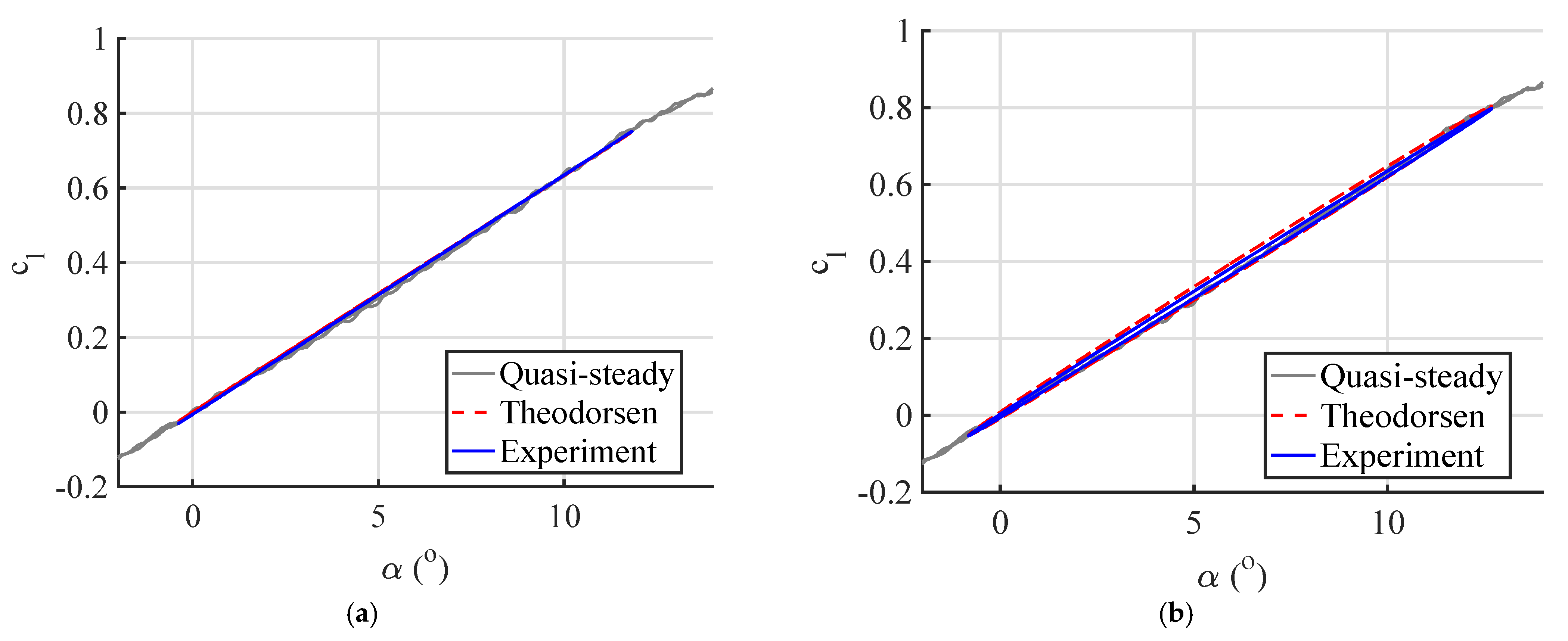
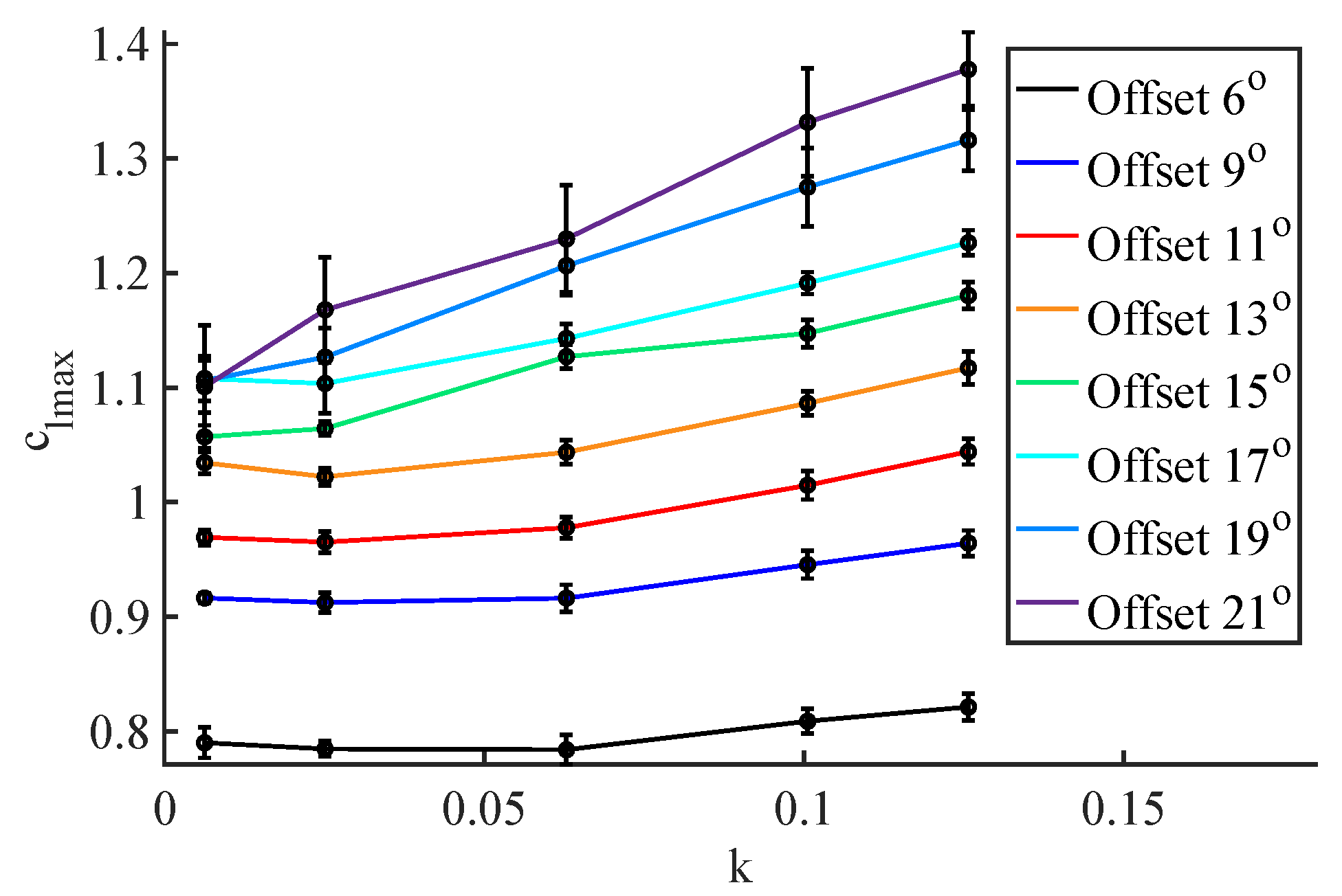
4. Quasi-Static Experiments

The first set of experiments was to obtain a characteristic quasi-static lift curve: aerodynamic lift force against the pitch angle. This curve revealed the basic flow features and provided a baseline for the dynamic tests. The quasi-static curve was obtained by slowly moving the wing as

$$\alpha ={\alpha }_o+{\alpha }_m\sin \left(2\pi ft\right)$$

(5)

where α_o is the pitch offset (set to 0°); α_m is the pitch amplitude (set to 28°); and the excited frequency (f) is 0.01 Hz, which corresponds to a reduced frequency (k) of 0.0006. The quasi-static curve for the positive pitch angles is shown in Figure 7. The curve was obtained by averaging three periods. The standard deviation of the data is shown as the shaded region. Three different regions can be broadly identified from the lift curve.

There was a linear region for α < 12° where the lift increased proportionally with the pitch angle. Above 12°, the lift curve slope decreased due to partial boundary layer separation originating at the trailing edge. Beyond 16°, the lift curve followed a different path for pitch up and pitch down, so-called lift hysteresis. This hysteresis region shows that even at low reduced frequencies, the lift is a nonlinear function of the angle of attack. Above 22°, the boundary layer fully separated from the suction side, and we observed a fully stalled region during both the pitch up and ensuing pitch down motion.

The wing was mounted in a cantilever position from the wind tunnel sidewall. Since there is no end-plate at the wing tip, the flow will leak from the high-pressure side to the low-pressure side of the wing at the tips. This will create tip vortices and the energy dissipated from these vortices will have a toll on the wing lift. Thus, the lift curve slope of the wing will be lower than that of an airfoil. For lower aspect ratio (AR) wings, the Helmbold equation can be used to calculate the lift curve slope [40]:

$$a=\frac{\pi AR}{1+\sqrt{1+{\left(\frac{AR}{2}\right)}^2}}$$

(6)

The Helmbold equation gives the theoretical slope as 3.7 (the black line in Figure 7), which is quite close to the estimated lift curve slope of the wing (a slope of 3.63, see the colored lines in Figure 7). Gudmundsson [41] compared different relations for correcting the lift curve slope for different aspect ratios and wing shapes and found that the Helmbold equation agreed well with experimental data.

The laminar separation bubble (LSB) plays an important part in determining the character of the boundary layer, the stalling characteristics of the wing, and the lift hysteresis. The LSB is formed when the laminar boundary layer separates over the wing surface due to the adverse pressure gradient downstream of the point of minimum pressure. A schematic diagram of the LSB and its determination from the pressure data can be found in [42]. They showed a schematic diagram (reprinted here as Figure 8 for clarity) detailing the formation of the LSB. ‘S’ indicates the point of separation. Downstream of the separation point, a laminar shear layer is formed, separating the streamline flow and the reverse flow between the boundary layer and the wing surface. The flow inside the shear layer is unstable and the transition from laminar to turbulent flow takes place. The transition starts at ‘T’, a short distance downstream of ‘S’, and converts into a fully turbulent flow at ‘T’. After the complete transition at ‘T’, the large turbulent shear stresses energize the separated shear layer by entraining fluid from the external stream so that it grows rapidly, causing the pressure to rise. Reattachment occurs at point ‘R’ when the pressure is nearly equal to the value for the turbulent boundary layer over the wing with no separation bubble present, as shown in Figure 8. The region between separation and reattachment is referred to as the laminar separation bubble. The fluid in the laminar portion (between ‘S’ and ‘T’) of the bubble moves very slowly, while the fluid in the turbulent portion (between ‘T’ and ‘R’) moves vigorously in a recirculating pattern.

The LSB could also be observed in our pressure data for the quasi-static case. The pressure coefficient c_p at different pitch angles for the pitch-up and pitch-down motion is shown in Figure 9. Different events on the lift curve are shown in numerals. Until point ‘1’, the lift curve was linear, and the lift was mostly due to the pressure drop on the suction side near the leading edge. After point ‘1’, a decrease in lift curve was observed, which indicates the start of the boundary layer separation from the trailing edge. Since we had no pressure tap after 77% of the chord, the trailing edge separation was not visible in the pressure data. We can see the formation of LSB at points ‘2’, ‘3’, and ‘4’, indicated as a circle in Figure 9. The separation, transition, and reattachment points can be identified similar to Figure 8. Point ‘5’ indicates the region of the full boundary layer separation from the suction side, as shown by a constant pressure distribution in the c_p plots. Pitching down, starting from a fully separated flow, no LSB was formed that would boost reattachment. This resulted in a different, lower lift force during pitch-down between 24° and 16° (flow reattachment) than that obtained during pitch-up. The points ‘2’ and ‘8’, ‘3’ and ‘7’, and ‘4’ and ‘6’, respectively, are snapshots at the same pitch angles. Their differences clearly demonstrate the presence of the lift hysteresis and how it is linked to the presence (pitch-up) or absence (pitch-down) of the LSB.

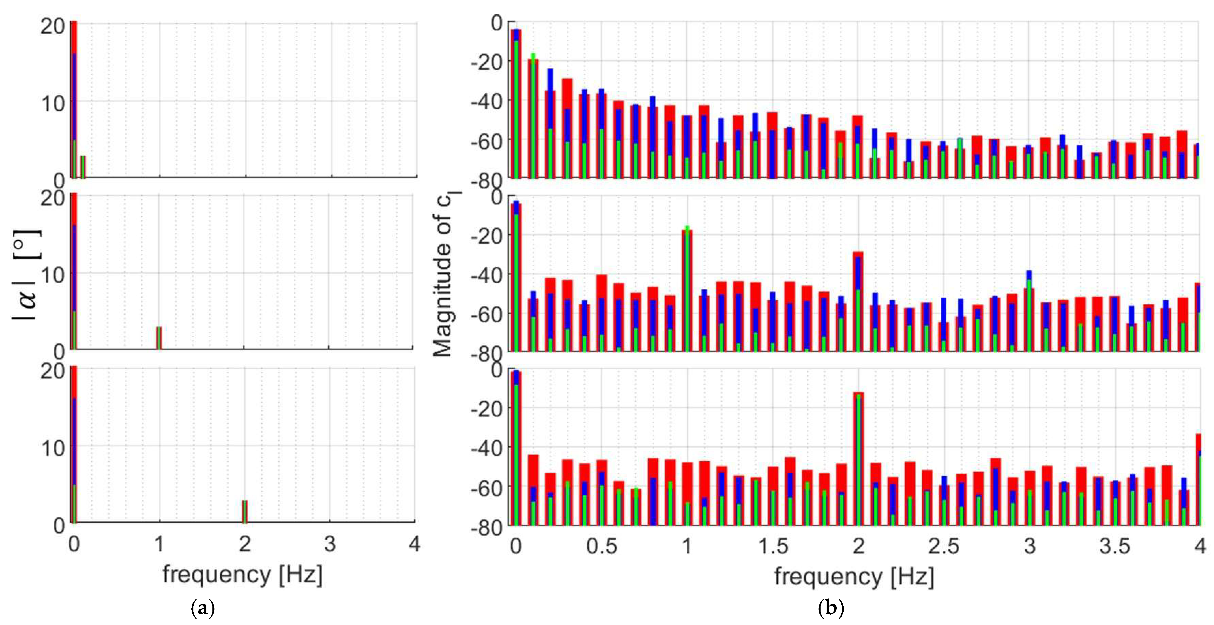
5. Monosine Experiments

Most of the work on understanding the unsteady motion of the wing involves harmonically pitching the wing [21,22,25,43,44]. In this work, we conducted experiments using simple harmonic sines (monosines) at different pitch offset angle, amplitude, and reduced frequencies. The list of all monosine experiments is given in

Table 2. Summary of the monosine experiments performed at different parameters.

Motion Type	Pitch Amplitude	Pitch Offset	k
Single sine	$\approx$6	6, 9, 11, 13, 15, 17, 19, 21	0.006, 0.025, 0.063, 0.101, 0.126

. The pitch amplitude was fixed at 6° and the pitch offset was gradually increased in steps. At each offset angle, the wing was pitched with five different single-sine frequencies that corresponded to a reduced frequency of 0.0063, 0.025, 0.063, 0.101, and 0.126.

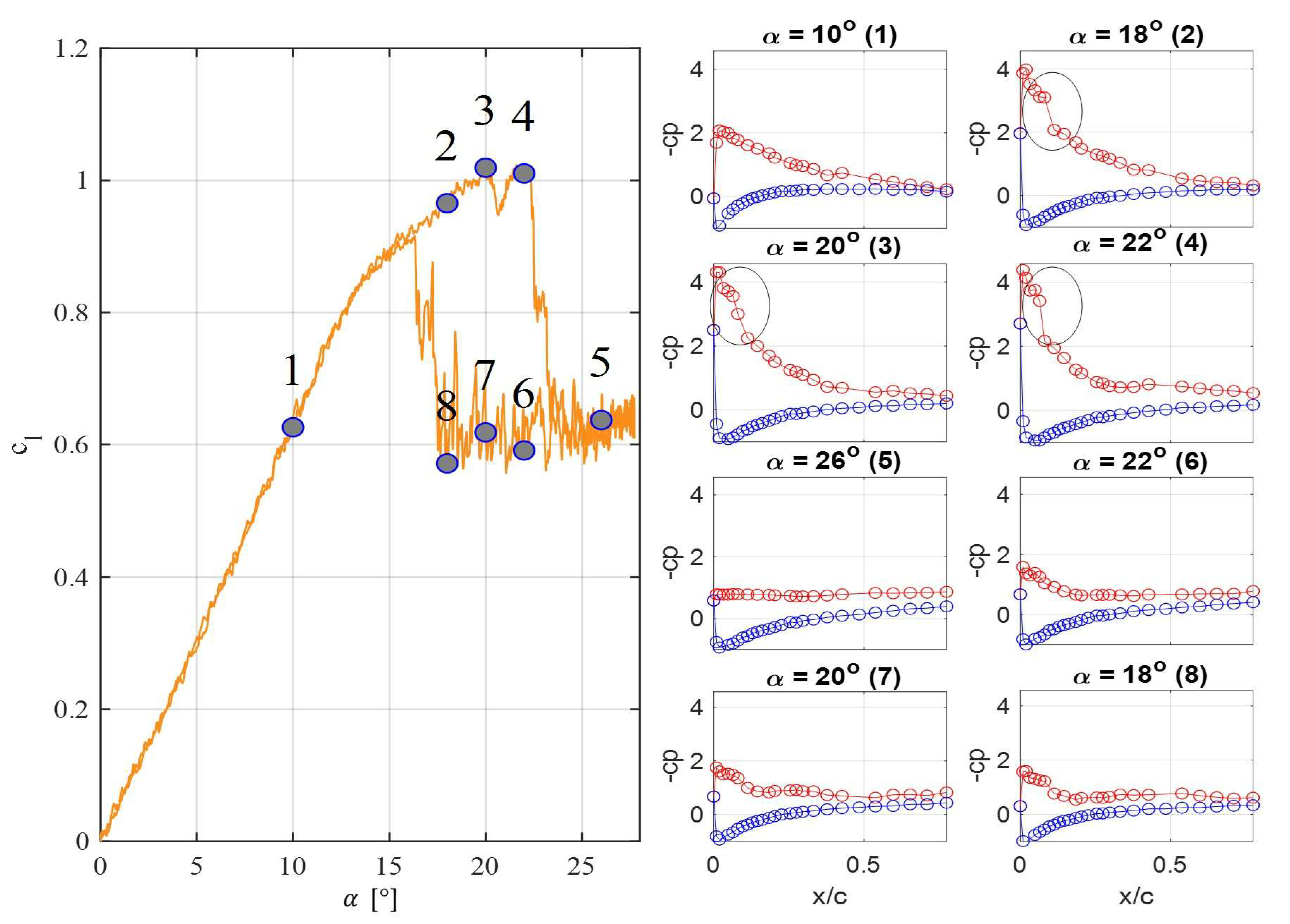
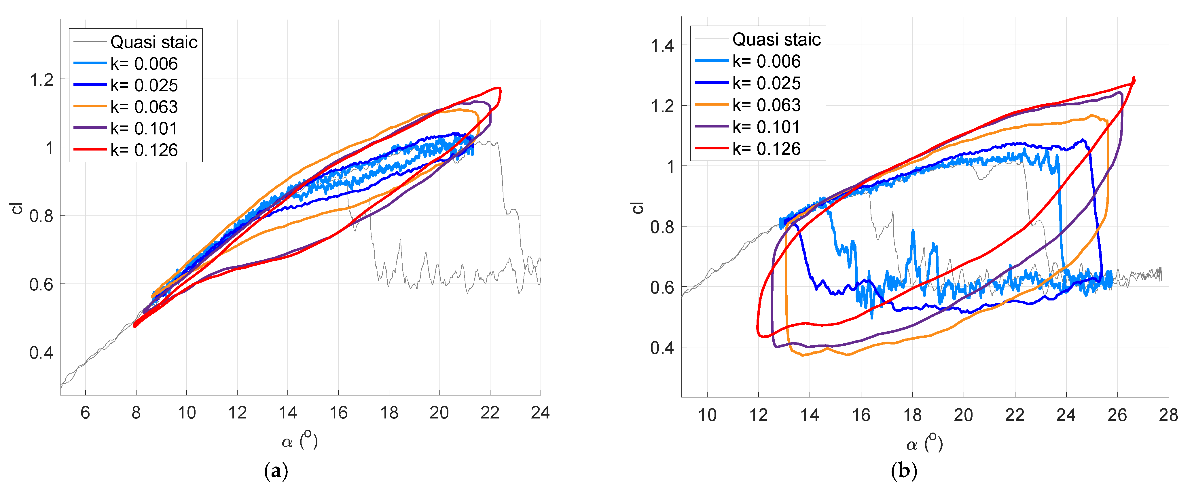
5.1. Aerodynamic Viewpoint

In Figure 10, the lift forces for different monosine experiments are shown for each of the offset angles. The curves for each reduced frequency were superimposed to illustrate the effect of increasing the pitch rate on the lift characteristics. The quasi-static curve was also plotted for comparison. To ease the discussion on the results, we focused on the results at the pitch offset of 6°, 15°, and 19° to cover the three regions identified in Section 4.

At the lower offset angle (6°), the curves for different reduced frequencies mostly fell on the quasi-static curve. The c_l variation with pitch angle is shown for the lowest and the highest reduced frequency in Figure 11. The experimental results were filtered to consider power only on the excited frequency line. This allowed us to compare the results with the linear unsteady relation of Theodorsen [13]. Since the Theodorsen model is derived from quasi-steady thin airfoil theory, it is valid only for airfoils [45]. Therefore, we adjusted the lift curve slope to match the actual (measured) slope for the wing. The experimental forces were in good agreement with the predictions from Theodorsen’s model.

At the offset angle of 15°, since the maximum pitch angle now exceeded the static stall angle, we observed hysteresis loops that grew with increasing reduced frequency (see Figure 10a). This was due to the formation of a leading-edge vortex (LEV) near the leading edge on the suction side of the wing. The strength of the LEV was increased with the favorable upward motion of the wing. This delayed the boundary layer separation and increased the maximum cl. However, during the downward motion, the LEV is shed, and the same principle now keeps the boundary layer separated longer. Therefore, a hysteresis loop is formed, which increases with reduced frequency.

At higher offset angles still (19°), reattachment did not occur during the downward motion, but near (or just past) the minimum angle of attack, as shown in Figure 10b. The ensuing increase in the size of the hysteresis loop can be attributed to the formation of a dynamic stall vortex (DSV). The DSV produces a localized drop in the suction pressure near the leading edge and results in a rapid rise in the lift. The strength of the DSV increases with the increase in the pitch rate. As the DSV sheds and traverses downstream, the leading-edge suction peak collapses, resulting in lift stall. The presence of the DSV was confirmed by the small kink near the maximum cl, especially at higher reduced frequencies [43].

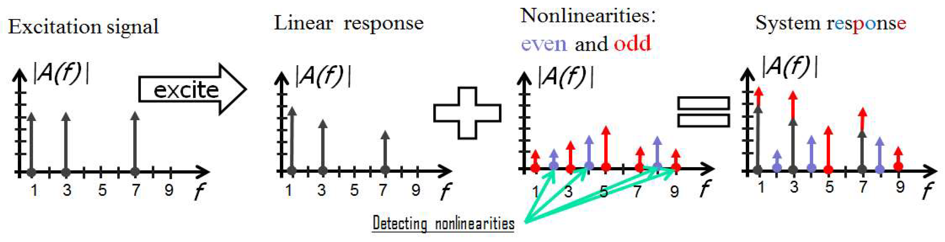
5.2. Vibro-Acoustic Viewpoint

The complex aerodynamic lift force for a harmonically pitching wing can also be seen as a classical nonlinear signal processing problem, not unlike a nonlinear vibro-acoustic system [36,46]. We explore that viewpoint in the present section to determine what (data-driven) model would be required to capture such nonlinear dynamics.

For most mechanical systems, small excitation levels lead to small, negligible nonlinear effects hidden in the noise. This corresponded in our case to the low offset angle of attack regions seen in Figure 11. When the excitation level increased, the nonlinearities tended to appear (as it is shown in Figure 10).

Figure 12 illustrates how a system response consists of a linear and nonlinear part in the frequency domain using a generic scenario. The major difference between the pitching wing problem and the classical mechanical/vibro-acoustic engineering applications is that the higher excitation level does not require an increase in the injected energy at all excited frequencies. More precisely, by increasing the offset angle of attack, we effectively only increased the energy of the DC (0 Hz) component.

For a monosine excitation, we thus did not increase the amplitude of the sine wave (i.e., the energy at the non-zero excited frequency, which would be the intuitive step) but the pitch offset angle while keeping the higher frequency component constant. This implies moving the range of the excitation by moving the mean value of the sine wave. With this excitation technique, we tested multiple points on the static curve, as illustrated in Figure 9.

To make the results more accessible, in the next figure, the frequency-domain input–output signals are shown at three offset angles: at 6° (low level), 15° (medium level), and 19° (high level), and at the excitation frequencies of 0.1 Hz (k = 0.006), 1 Hz (k = 0.063), and 2 Hz (k = 0.126), respectively. The input (angle of attack) measurements are shown in Figure 13a. We observed that the excitation signals were almost identical; the only significant difference could be found at 0 Hz: the mean (offset) value of the pitch angle (comparing the green (low), blue (medium), and red (high) bars at 0 Hz).

The post-processed output (lift coefficient) measurements are shown in Figure 13b. The level-wise spectral characteristics varied with the excitation levels, even in the nonexcited frequency band, as could be expected for a nonlinear system. The output/input ratio varied: the higher the level of excitation, the higher the energy injected at and around the frequency bin of the excitation line. These output/input ratios at the excited (non-zero) frequency lines are also a function of the frequency and the excitation level. This means that the system indeed shows complex nonlinear dynamical behavior; an appropriate (data-driven) model should thus be able to represent a (strongly) nonlinear and dynamic system. A detailed frequency domain analysis of the pitching wing using broadband excitation can be found in [5,6,47].

One way to illustrate the importance of the nonlinear dynamics of a pitching wing is through the variation in the maximum lift force with reduced frequency for different pitch offsets. This is shown in Figure 14 for all the experiments listed in Table 2. The curves for which the maximum pitch angle exceeded the static stall angle displayed a steeper rise in the maximum c_l.

6. Conclusions

The unsteady lift force on a pitching wing plays an important role in many engineering problems in aeronautics and wind energy. Often, empirical models are used to predict the lift force as a function of a (harmonically) varying angle of attack. From a vibro-acoustic viewpoint, the unsteady aerodynamic force acts as a spring, albeit a strongly nonlinear one. A small-order model that captures the salient (nonlinear) characteristics of the aerodynamic force would greatly improve the existing tools (such as digital twins) for design optimization or for real-time control.

This work demonstrates unsteady measurement on a low aspect ratio pitching wing to allow for the construction of data-driven small-order models. However, the experimental setup used for the experiments posed unique measurement challenges that were addressed in the post-processing using advanced signal processing techniques.

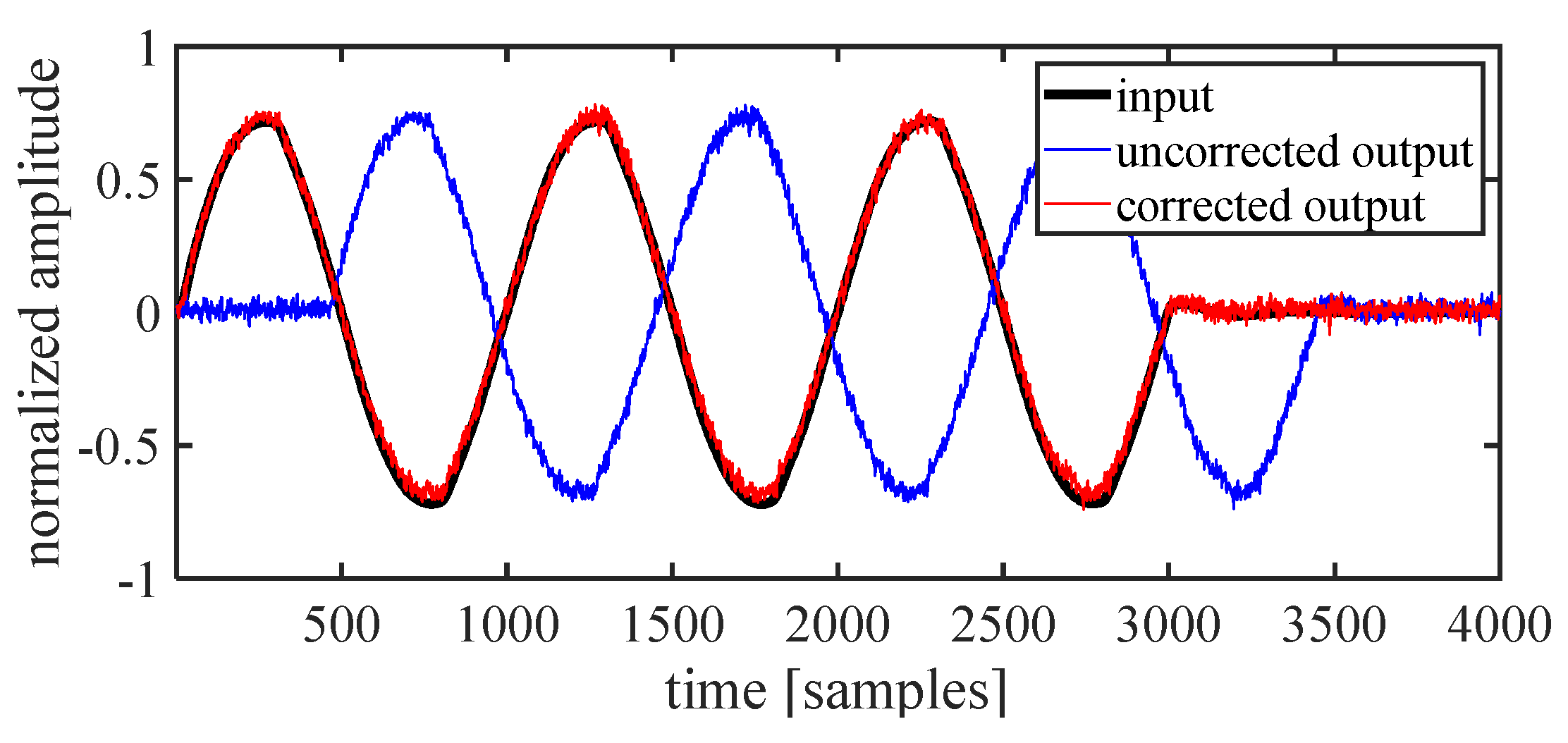
• The lack of synchronization was solved through a so-called starting signal specifically constructed for the proper synchronization of the pitch angle and lift force data. This allowed for synchronization of the two datasets with an accuracy of <5 ms.
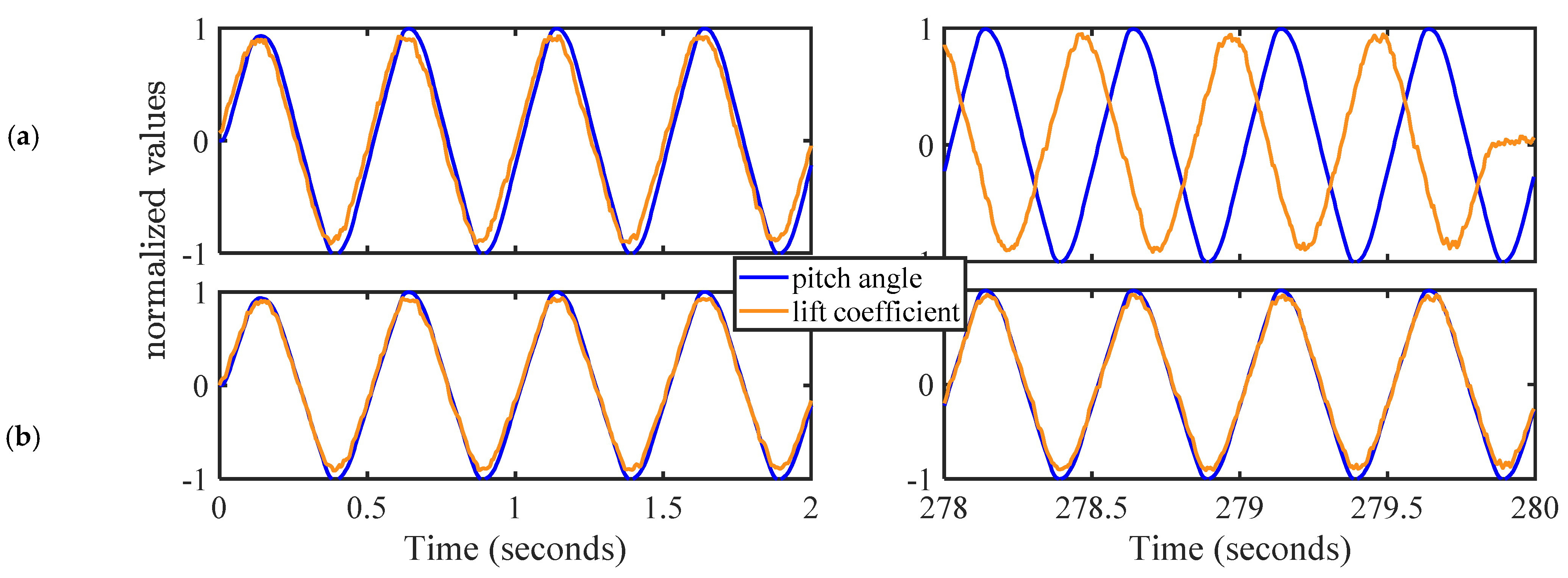
• The faulty clock frequency of the pressure measurement DAQ was determined through a fully automated spectral analysis tool that estimates the period time of a periodic signal for a given sampling frequency. The analysis revealed that the correct sampling frequency of the DAQ was 199.88 Hz instead of 200 Hz.

The quasi-steady experiments showed a bi-stable behavior at higher pitch angles, also termed as static hysteresis. The pressure distribution on the suction side revealed the formation of a leading-edge separation bubble (LESP); the hysteresis behavior was attributed to the formation and bursting of the LESP during the pitch-up motion of the wing.

Unsteady (harmonic) measurements at different offset levels revealed that the wing behaves in a linear dynamic fashion at lower pitch offsets. The results agree with the theoretical (linear) unsteady models corrected for the low wing aspect ratio. At higher pitch offsets, beyond stall, the maximum lift force varies dynamically due to the formation of dynamic stall vortex (DSV). Indeed, the strength of the DSV (which influences the lift force) grows nonlinearly with an increase in reduced frequency. Therefore, proper modeling of the unsteady lift force on a pitching wing necessitates the use of a nonlinear dynamic model.

References

- Mueller, T.J. Fixed and Flapping Wing Aerodynamics for Micro Air Vehicle Applications; American Institute of Aeronautics and Astronautics: Reston, VA, USA, 2001. [Google Scholar]
- Ansari, S.A.; Żbikowski, R.; Knowles, K. Non-linear unsteady aerodynamic model for insect-like flapping wings in the hover. Part 2: Implementation and validation. Proc. Inst. Mech. Eng. Part G J. Aerosp. Eng. 2006, 220, 169–186. [Google Scholar] [CrossRef] [Green Version]
- Leishman, J.G. Challenges in modelling the unsteady aerodynamics of wind turbines. Wind Energy Int. J. Prog. Appl. Wind Power Convers. Technol. 2002, 5, 85–132. [Google Scholar] [CrossRef]
- De Troyer, T.; Hasin, D.; Keisar, D.; Santra, S.; Greenblatt, D. Plasma-Based Dynamic Stall Control and Modeling on an Aspect-Ratio-One Wing. AIAA J. 2022, 60, 2905–2915. [Google Scholar] [CrossRef]
- Siddiqui, M.; De Troyer, T.; Decuyper, J.; Csurcsia, P.; Schoukens, J.; Runacres, M. A data-driven nonlinear state-space model of the unsteady lift force on a pitching wing. J. Fluids Struct. 2022, 114, 103706. [Google Scholar] [CrossRef]
- De Troyer, T.; Csurcsia, P.Z.; Siddiqui, M.F.; Runacres, M. Using a broadband multisine excitation signal for the data-driven modeling of the unsteady lift force on a pitching wing. In Proceedings of the 2022 ISMA International Conference on Noise and Vibration Engineering, Leuven, Belgium, 12–14 September 2022. [Google Scholar]
- Balajewicz, M.; Dowell, E. Reduced-order modeling of flutter and limit-cycle oscillations using the sparse Volterra series. J. Aircr. 2012, 49, 1803–1812. [Google Scholar] [CrossRef]
- Beddoes, T.S. A Qualitative Discussion of Dynamic Stall; AGARD Special Course on Unsteady Aerodynamics, AGARD Report 679; Advisory Group for Aerospace Research and Development: London, UK, 1979. [Google Scholar]
- Patil, M.J.; Hodges, D.H. On the importance of aerodynamic and structural geometrical nonlinearities in aeroelastic behavior of high-aspect-ratio wings. J. Fluids Struct. 2004, 19, 905–915. [Google Scholar] [CrossRef]
- Rockwood, M.; Medina, A.; Garmann, D.J.; Visbal, M.R. Dynamic Stall of a Swept Finite Wing for a Range of Reduced Frequencies. In Proceedings of the AIAA Aviation 2019 Forum, Dallas, TX, USA, 17–21 June 2019. [Google Scholar] [CrossRef]
- Ertveldt, J.; Pintelon, R.; Vanlanduit, S. Identification of Unsteady Aerodynamic Forces from Forced Motion Wind Tunnel Experiments. AIAA J. 2016, 54, 3265–3273. [Google Scholar] [CrossRef]
- Ertveldt, J.; Lataire, J.; Pintelon, R.; Vanlanduit, S. Frequency-domain identification of time-varying systems for analysis and prediction of aeroelastic flutter. Mech. Syst. Signal Process. 2014, 47, 225–242. [Google Scholar] [CrossRef]
- Theodorsen, T. General Theory of Aerodynamic Instability and the Mechanism of Flutter; National Advisory Committee for Aeronautics: Washington, WA, USA, 1979. [Google Scholar]
- Razak, N.A.; Andrianne, T.; Dimitriadis, G. Flutter and Stall Flutter of a Rectangular Wing in a Wind Tunnel. AIAA J. 2011, 49, 2258–2271. [Google Scholar] [CrossRef]
- Dimitriadis, G.; Li, J. Bifurcation Behavior of Airfoil Undergoing Stall Flutter Oscillations in Low-Speed Wind Tunnel. AIAA J. 2009, 47, 2577–2596. [Google Scholar] [CrossRef]
- Dimitriadis, G. Introduction to Nonlinear Aeroelasticity; Wiley: New York, NY, USA, 2017. [Google Scholar]
- Deparday, J.; Mulleners, K. Modeling the interplay between the shear layer and leading edge suction during dynamic stall. Phys. Fluids 2019, 31, 107104. [Google Scholar] [CrossRef]
- Schreck, S.J.; Hellin, H.E. Unsteady vortex dynamics and surface pressure topologies on a finite pitching wing. J. Aircr. 1994, 31, 899–907. [Google Scholar] [CrossRef]
- Wernert, P.; Geissler, W.; Raffel, M.; Kompenhans, J. Experimental and numerical investigations of dynamic stall on a pitching airfoil. AIAA J. 1996, 34, 982–989. [Google Scholar] [CrossRef]
- Okamoto, M.; Azuma, A. Experimental Study on Aerodynamic Characteristics of Unsteady Wings at Low Reynolds Number. AIAA J. 2005, 43, 2526–2536. [Google Scholar] [CrossRef]
- Kaufmann, K.; Merz, C.B.; Gardner, A.D. Dynamic stall simulations on a pitching finite wing. J. Aircr. 2017, 54, 1303–1316. [Google Scholar] [CrossRef]
- Angulo, I.A.; Ansell, P.J. Influence of Aspect Ratio on Dynamic Stall of a Finite Wing. AIAA J. 2019, 57, 2722–2733. [Google Scholar] [CrossRef]
- Visbal, M. Flow Structure and Unsteady Loading over a Pitching and Perching Low-Aspect-Ratio Wing. In Proceedings of the 42nd AIAA Fluid Dynamics Conference and Exhibit, New Orleans, LA, USA, 25 June 2012. [Google Scholar] [CrossRef]
- Visbal, M.R.; Garmann, D.J. Effect of Sweep on Dynamic Stall of a Pitching Finite-Aspect-Ratio Wing. AIAA J. 2019, 57, 3274–3289. [Google Scholar] [CrossRef]
- Visbal, M.R.; Garmann, D.J. Dynamic stall of a finite-aspect-ratio wing. AIAA J. 2019, 57, 962–977. [Google Scholar] [CrossRef]
- Spentzos, A.; Barakos, G.; Badcock, K.; Richards, B.; Wernert, P.; Schreck, S.; Raffel, M. Investigation of Three-Dimensional Dynamic Stall Using Computational Fluid Dynamics. AIAA J. 2005, 43, 1023–1033. [Google Scholar] [CrossRef] [Green Version]
- Spentzos, A.; Barakos, G.N.; Badcock, K.J.; Richards, B.E.; Coton, F.N.; Galbraith, R.M.; Berton, E.; Favier, D. Computational fluid dynamics study of three-dimensional dynamic stall of various planform shapes. J. Aircr. 2007, 44, 1118–1128. [Google Scholar] [CrossRef]
- Hoerner, S.F.; Borst, H.V. Fluid-Dynamic Lift: Practical Information on Aerodynamic and Hydrodynamic Lift; LA Hoerner: New York, NY, USA, 1985. [Google Scholar]
- Chinwicharnam, K.; Ariza, D.G.; Moschetta, J.-M.; Thipyopas, C. Aerodynamic Characteristics of a Low Aspect Ratio Wing and Propeller Interaction for a Tilt-Body MAV. Int. J. Micro Air Veh. 2013, 5, 245–260. [Google Scholar] [CrossRef] [Green Version]
- Aboelezz, A.; Hassanalian, M.; Desoki, A.; Elhadidi, B.; El-Bayoumi, G. Design, experimental investigation, and nonlinear flight dynamics with atmospheric disturbances of a fixed-wing micro air vehicle. Aerosp. Sci. Technol. 2020, 97, 105636. [Google Scholar] [CrossRef]
- Timmer, W. Two-dimensional low-Reynolds number wind tunnel results for airfoil NACA 0018. Wind Eng. 2008, 32, 525–537. [Google Scholar] [CrossRef] [Green Version]
- Bhandari, P.; Csurcsia, P.Z. Digital implementation of the PID controller. Softw. Impacts 2022, 13, 100306. [Google Scholar] [CrossRef]
- Bergh, H.; Tijdeman, H. Theoretical and Experimental Results for the Dynamic Response of Pressure Measuring Systems; National Aero and Astronautical Research Institute: Amsterdam, The Netherlands, 1965. [Google Scholar]
- Csurcsia, P.Z.; Lataire, J. Nonparametric estimation of time-varying systems using 2-D regularization. IEEE Trans. Instrum. Meas. 2016, 65, 1259–1270. [Google Scholar] [CrossRef]
- Csurcsia, P.Z.; Peeters, B.; Schoukens, J. User-friendly nonlinear nonparametric estimation framework for vibro-acoustic industrial measurements with multiple inputs. Mech. Syst. Signal Process. 2020, 145, 106926. [Google Scholar] [CrossRef]
- Csurcsia, P.Z.; Peeters, B.; Schoukens, J.; De Troyer, T. Simplified analysis for multiple input systems: A toolbox study illustrated on F-16 measurements. Vibration 2020, 3, 70–84. [Google Scholar] [CrossRef] [Green Version]
- Csurcsia, P.Z.; Peeters, B.; Schoukens, J. The best linear approximation of MIMO systems: Simplified nonlinearity assessment using a toolbox. In Proceedings of the International Conference on Noise and Vibration Engineering 2020, Leuven, Belgium, 12–14 September 2022; pp. 2239–2252. [Google Scholar]
- Schoukens, J.; Rolain, Y.; Simon, G.; Pintelon, R. Fully automated spectral analysis of periodic signals. IEEE Trans. Instrum. Meas. 2003, 52, 1021–1024. [Google Scholar] [CrossRef]
- Wickens, R. Wind Tunnel Investigation of Dynamic Stall of an NACA 0018 Airfoil Oscillating in Pitch (Etude en Soufflerie du Decrochage Aerodynamique d’un Profil NACA 0018 Oscillant en Tangage); National Aeronautical Establishment: Ottawa, ON, Canada, 1985. [Google Scholar]
- Stengel, R.F. Flight Dynamics; Princeton University Press: Princeton, NJ, USA, 2015. [Google Scholar] [CrossRef]
- Gudmundsson, S. General Aviation Aircraft Design: Applied Methods and Procedures; Butterworth-Heinemann: Oxford, UK, 2013. [Google Scholar]
- Arena, A.V.; Mueller, T.J. Laminar Separation, Transition, and Turbulent Reattachment near the Leading Edge of Airfoils. AIAA J. 1980, 18, 747–753. [Google Scholar] [CrossRef]
- Coton, F.; Galbraith, R. An examination of dynamic stall on an oscillating rectangular wing. In Proceedings of the 21st AIAA Applied Aerodynamics Conference, Orlando, FL, USA; 2003; p. 3675. [Google Scholar]
- Ullah, A.H.; Tomek, K.L.; Fabijanic, C.; Estevadeordal, J. Dynamic Stall Characteristics of Pitching Swept Finite-Aspect-Ratio Wings. Fluids 2021, 6, 457. [Google Scholar] [CrossRef]
- Brunton, S.L.; Rowley, C.W. Empirical state-space representations for Theodorsen’s lift model. J. Fluids Struct. 2013, 38, 174–186. [Google Scholar] [CrossRef]
- Csurcsia, P.Z. User-Friendly Method to Split Up the Multiple Coherence Function Into Noise, Nonlinearity and Transient Components Illustrated on Ground Vibration Testing of an F-16 Fighting Falcon. J. Vib. Eng. Technol. 2022, 10, 2577–2591. [Google Scholar] [CrossRef]
- Siddiqui, M.F.; Decuyper, J.; Csurcsia, P.Z.; Ertveldt, J.; De Troyer, T.; Schoukens, J.; Runacres, M.C. Estimating a nonparametric data-driven model of the lift on a pitching wing. J. Phys. Conf. Ser. 2020, 1618, 05201. [Google Scholar] [CrossRef]