Article

Free and Forced Vibration Behaviors of Magnetodielectric Effect in Magnetorheological Elastomers

Department of Mechanical, Industrial and Aerospace Engineering, Concordia University, Montréal, QC H3G 1M8, Canada
*
Authors to whom correspondence should be addressed.
Vibration 2023, 6(1), 269-285; https://doi.org/10.3390/vibration6010017
Submission received: 29 January 2023 / Revised: 22 February 2023 / Accepted: 1 March 2023 / Published: 3 March 2023

Abstract

:
This paper is concerned with the free and forced vibration responses of a magneto/electroactive dielectric elastomer, emphasizing the chaotic phenomena. The dielectric elastomers under external magnetic and electrical excitations undergo large elastic deformation. The magnetodielectric elastomer is modeled based on the Gent–Gent strain energy function to incorporate the influence of the second invariant and the strain stiffening. The viscoelasticity of the active polymer is also considered in the form of Rayleigh’s dissipation function. The equation of motion is governed with the aid of the Lagrangian equation in terms of a physical quantity, namely, the stretch of the elastomer. An energy-based approach is utilized to re-evaluate the static and DC voltage instabilities of the resonator. Time-stretch response (time history behavior), phase plane diagram, Poincaré map, and fast Fourier transform are numerically obtained and presented to explore the chaotic oscillation behavior of the active polymer actuators. The results reveal that the magnetic field may tune the stability and instability regions of the active polymeric membrane. It has also been shown that the applied magnetic field may lead to chaotic vibration responses when a sinusoidal voltage is applied simultaneously to the system. The results presented in this paper can be effectively used to design magnetic and electrical soft robotic actuators and elastomer membranes under electrical and magnetic stimulants.

1. Introduction

Active polymers are smart-functional materials capable of altering their mechanical and geometrical properties under the application of external physical stimuli [1]. These external stimuli may be electrical [2], light [3], thermal [4], magnetic [5,6], and hygrothermal [7]. All these excitation methods have provided new routes into the design of smart systems that can be mechanically responsive and adaptive to environmental changes. There are some limitations associated with the practical applications of some active materials. For instance, light-activated materials are limited by the opaqueness of the surrounding area, while thermal and hygrothermal active materials may require local environmental conditions and provide slow responses to external excitations and thus not applicable for real-time control applications. In these concerns, magneto/electroactive materials, due to their fast response and the possibility of remote actuation, can potentially overcome these limitations and become ideal candidates for several applications within soft robotics actuators and smart sensors [8,9]. Magnetodielectric elastomers (MDEs) have properties of both magnetoactive material and dielectric elastomer (DE) and are thus responsive to both magnetic and electrical loads [10,11]. The magnetodielectric effect has received recent interest due to its capability to control the dielectric permittivity in response to applied magnetic fields. Materials showing a significant magnetodielectric effect are suitable for new applications, including radio frequency, tunable microwaves, filters, four-state memories, magnetic sensors, and spin-charge transducers [12,13,14]. Magnetodielectric nanocomposite materials based on nanoparticles with polyvinylidene fluoride (PVDF) and polydimethylsiloxane (PDMS) were used for antenna applications [15,16]. Yang et al. [17] reported that the dielectric permittivity of the polymer composite increases with the increasing amount of Fe3O4 doping and is not influenced by nanoparticle size. Isaev et al. [10] presented the results of the numerical simulation of the magnetodielectric effect of three types of particle size distributions on magnetorheological elastomers. It is notable that the majority of studies in this area were focused on the effect of the volume content of particles on the dielectric response and magnetization. Stojak et al. [13] investigated tunable magnetodielectric polymers. They showed that these materials might experience large deformation unsuitable for applications such as microwave metamaterials and magnetic sensors. Thus, knowing the free and forced vibration behaviors of magnetoactive materials and electroactive elastomers is essential for their design and practical application.
Polymers stimulated by electrical excitation are called electroactive polymers (EAPs). The most well-known material in EAPs is dielectric elastomers (DEs). DEs deform under the application of an electrical field and show large deformation and strain [18,19]. Static and dynamic responses of DEs with different geometries have been well addressed. For example, Zhu et al. [20] investigated the dynamic response of a spherical DE using the neo-Hookean model. They obtained the equation of motion for the system using the method of virtual work and solved the problem numerically and analytically. Sheng et al. [21] analyzed the nonlinear oscillation of a rectangular DE membrane using virtual work and utilizing the Gent hyperelastic material model. Wang et al. [22] studied a circular DE’s static and dynamic characteristics using the Gent model and Lagrangian equation. Different models have been utilized to investigate the time and frequency response of microbeams made of DEs, such as the neo-Hookean, Gent, and Cosserat hyperelastic models [23,24]. Several research studies investigated the static and dynamic behaviors of fiber-reinforced DEs. Hyperelastic models such as neo-Hookean, Gent, Mooney–Rivlin, and Ogden were generally used [25,26]. Recently, Alibakhshi et al. [27] showed that multi-frequency excitation could control the effect of the damping in the system and improve the performance of dielectric elastomers, where a higher response amplitude is required. To the best of our knowledge, some papers considered the experimental analysis of the simultaneous effect of both electrical and magnetic stimuli [28,29]. However, no study has been conducted on the simultaneous chaotic effect of both electrical and magnetic stimuli on the performance of the dielectric elastomers and their dynamic response behavior.
As mentioned above, the magnetic field can be effectively used to actuate some active polymers [30,31,32]. The study of magnetoactive polymers (MAPs) is a growing field of study worldwide due to their potential widespread biomedical applications, and use in soft robotics and adaptive smart systems [33,34]. They can also be custom-made fabricated using the novel 3D and 4D printing technologies [35,36]. The theory and fundamental formulations of MAPs were nearly developed three decades ago when Dorfmann et al. [37] extended the electromagnetism theories for elastomers and polymers. Garcia-Gonzalez [38] extended the theory and applications of a magnetically actuated soft polymer (hard magnetic soft materials) using the neo-Hookean model. Zhao et al. [39] analyzed the mechanics of magneto/active soft polymers considering the magnetic field in the thickness direction and used the neo-Hookean model to capture the nonlinear nature of the polymer. Dorfman and Odgen [37] reported a detailed description and formulation of electro-magneto-active polymers. Kumar et al. [38] also provide a universal formulation of polymers triggered by electromagnetic excitations.
Similar to DEs, the static and dynamic responses of MAPs are of significant importance for their design and applications as actuators. For example, Khurana et al. [40] investigated the static and DC dynamic responses of an MAP using the Lagrangian equation. They also included the influence of the electric field. They used a molecular-based hyperelastic model to assess the influence of the polymer chain entanglements and crosslinks on the characteristics of the MAP. Haldar et al. [41] developed a finite element formulation of an MAP in the context of finite deformation (large deformation). Khurana and co-workers [42] later conducted a vibrational analysis of and depicted a phase plane diagram and Poincaré map to give more details about the system’s response. In another study, Xing and Yong [43] developed a dynamic model and a controller for a magnetically actuated polymer using the neo-Hookean constituent material model.
The literature review mentioned above shows that the chaotic responses of MAPs under the simultaneous application of both electrical and magnetic stimuli have not been investigated. More specifically, the influence of the magnetic field on the chaos and stability of active polymers needs more investigation. This study aims to investigate the static and dynamic responses of MDEs. In the following, the first governing equations of motion are derived using the Lagrangian equation and solved numerically using the Runge–Kutta method. An energy method is subsequently expressed to analytically explore the static and dynamic instability of the magnetodielectric elastomer, and finally, the results are presented and discussed.

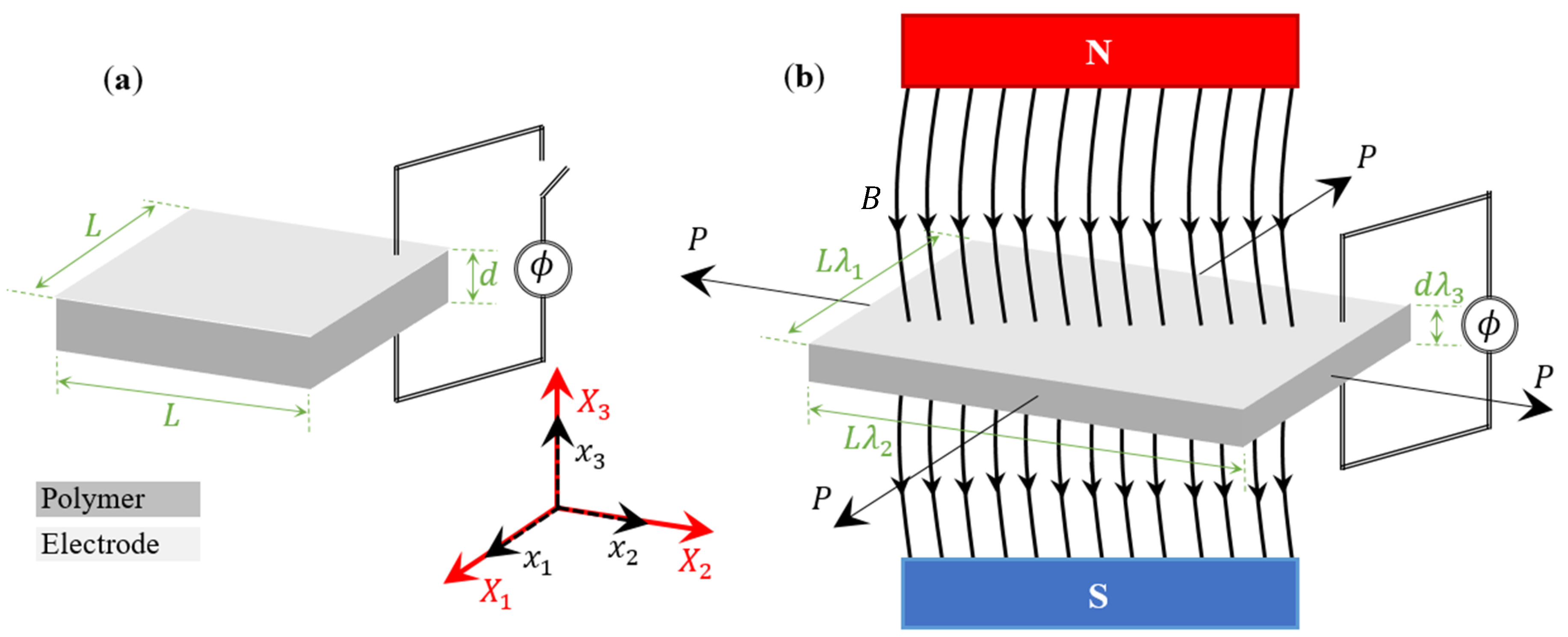
2. Mathematical Formulation

The schematic representation of a magneto-electro-active membrane is depicted in Figure 1. The length, width, and thickness of the membrane are denoted by L , L , and d , respectively. The continuum mechanics notation is utilized to derive equations of motion of the membrane undergoing large deformation. Thus, two configurations are set to define the deformation of the membrane. The first one is the reference (undeformed) configuration (Figure 1a), in which there are no applied forces to the membrane. The second one is the actuated (deformed) configuration (Figure 1b), where the membrane is subjected to magneto-electro-mechanical loading. A rectangular Cartesian coordinate system is used to specify the deformation of the system, which is X 1 , X 2 , X 3 in the reference configuration and x 1 , x 2 , x 3 in the actuated deformed configuration. In a deformed form, the membrane is subjected to in-plane mechanical load P , which may be static or harmonic, as well as external AC/DC magnetic ( B ) and electrical ( ϕ ) excitations.
The governing equations of motion are derived by assuming the following conditions:
  • The polymeric membrane is assumed to be incompressible, e.g., the volume of the reference and actuated model are equal.
  • The deformation of the membrane is specified in terms of the stretch λ .
  • It is assumed that the thickness of the membrane is thin (the inertia in the out-of-plane direction ( X 3 , x 3 ) is negligible); thus, only the in-plane deformation is analyzed.
  • Linear viscoelasticity is assumed using the Kelvin–Voigt model.
The stretches in x 1 , x 2 , x 3 directions can be represented as:
λ 1 = x 1 X 1 , λ 2 = x 2 X 2 , λ 3 = x 3 X 3 .
For the in-plane motion, it is assumed λ = λ 1 = λ 2 in which the stretch only depends on time, namely, λ = λ ^ t . Therefore, the equations of motion can be derived in terms of the stretch λ and its derivates. The governing equations of motion are derived using an energy approach based on the Euler–Lagrange equation:
d d t U K λ ˙ + U S λ = F λ ˙ + W P λ ,
in which U K stands for kinetic energy; U S is the potential energy; F refers to Rayleigh’s dissipation function; and W P is the work performed by external forces. The kinetic energy of the soft system membrane is formulated as follows:
U K = 1 2 ρ V x ˙ 1 + x ˙ 2 + x ˙ 3 d V ,
where V and ρ are the volume and density of the membrane. For the in-plane motion, x ˙ 3 is zero. Substituting Equation (1) into Equation (3) yields:
U K = 1 2 ρ 0 d 0 L 0 L λ ˙ 1 2 X 1 2 + λ ˙ 2 2 X 2 2 λ 1 λ 2 λ 3 = 1   d X 1 d X 2 d X 3 .
It is noted that λ 1 λ 2 λ 3 = 1 owing to the incompressibility constraint. Considering λ = λ 1 = λ 2 , Equation (4) can be simplified in terms of λ as:
U K = 1 3 ρ d L 4 d λ d t 2 + O d 3
The term O d 3 shows that only in-plane deformation has been included in the kinetic energy. The potential energy of the system under consideration may be described as:
U S = L 2 d ψ e l a s t i c + ψ e l e c t r i c a l + ψ m a g n e t i c .
where ψ e l a s t i c ,   ψ e l e c t r i c a l , and   ψ m a g n e t i c are elastic, electrical, and magnetic potential energies per unit volume. The elastic part of the potential energy is formulated using the Gent–Gent hyperelastic material model developed by Pucci and Saccomandi [44]. This model includes both the strain-stiffening effect and the second invariant and provides better performance compared with the classic Gent model for a broader range of deformation [45] and can be described with respect to the first and second invariants as [46]:
ψ e l a s t i c = C 1   J m 2 ln 1 I 1 3 J m + C 2 ln I 2 3 ,
in which C 1 and C 2 are material constants which are identified by experimental data, and J m represents a dimensionless parameter related to limiting stretch λ lim , which is called the Gent parameter (stiffening parameter) and measures the maximum available stretches of the membrane ( J m = 2 λ lim 2 + λ lim 4 3 ). I 1 and I 2 are the first and second principal invariants of the right Cauchy–Green deformation tensor, which are formulated as:
I 1 = i = 1 3 λ i 2 = 2 λ 2 + λ 4 , I 2 = i , j = 1 3 λ i λ j = λ 4 + 2 λ 2 .
Substituting Equation (8) into Equation (7), we can write the following relation for elastic potential energy with respect to the stretch, λ :
ψ e l a s t i c = C 1   J m 2 ln 1 2 λ 2 + λ 4 3 J m + C 2 ln λ 4 + 2 λ 2 3
The electrical potential energy can be expressed as:
ψ e l e c t r i c a l = ε E 2 λ 1 2 λ 2 2 = ε 2 ϕ d 2 λ 1 2 λ 2 2 = ε 2 ϕ d 2 λ 4
in which ε stands for the permittivity of the soft membrane; E = ϕ / d indicates the true electric field; and ϕ is the applied voltage to the electrodes attached at the top and bottom surfaces of the membrane. The potential energy of the magnetic force is also formulated as:
ψ m a g n e t i c = 1 2 μ B L . C B L
in which μ stands for the magnetic permeability; B L is the magnetic induction vector; and C is the right Cauchy–Green deformation tensor, which are expressed as:
C = λ 2 0 0 0 λ 2 0 0 0 λ 4 B L = 0 0 B B = μ H + M
In Equation (12), H is the reference magnetic field applied in the thickness direction, and M is the magnetic polarization density. Substituting Equation (12) into Equation (11) and considering the structure without magnetization, the potential energy for the magnetic field ( ψ m a g n e t i c ) is formulated as:
ψ m a g n e t i c = 1 2 μ H 2 λ 4
Finally, substituting Equations (9), (10), and (13) into Equation (6) yields the final potential energy as:
U S = L 2 d C 1   J m 2 ln 1 2 λ 2 + λ 4 3 J m + C 2 ln λ 4 + 2 λ 2 3 ε 2 ϕ H 2 λ 4 + 1 2 μ H 2 λ 4
The work performed by the in-plane tensile mechanical loads is formulated as:
W P = X 1 x 1 P d x 1 + X 2 x 2 P d x 2 = P λ L L + P λ L L = 2 P L λ 1
The damping of the membrane is captured with the aid of Rayleigh’s dissipation function, such that [47]:
F = 1 2 c d L 2 λ ˙ 2 ,
where c d is the viscous damping coefficient. Finally, considering Equations (14)–(16) and employing the Lagrangian equation, Equation (2), the governing equation of motion, is derived as:
1 3 ρ L 2 C 1     d 2 λ d t 2 + 1 2 c d C 1 d     d λ d t + J m λ λ 5 J m 2 λ 2 λ 4 + 3 + 2 C 2 λ 3 λ 3 C 1 2 λ 2 + λ 4 ε C 1 ϕ d 2 λ 3 μ H 2 C 1 λ 5 P C 1 L d = 0
Using the following dimensionless variables: nondimensional time τ = t / L ρ / 3 C 1 ; nondimensional damping coefficient c = c d / 2 C 1 L d ρ / 3 C 1 ; nondimensional mechanical load S ¯ = P / C 1 L d ; nondimensional voltage V ¯ = ε / C 1 ϕ / d ; nondimensional magnetic field H ¯ = μ / C 1 H and K = C 2 / C 1 , Equation (17) can be cast into the following dimensionless form:
λ ¨ + c λ ˙ + J m λ λ 5 J m 2 λ 2 λ 4 + 3 + 2 K λ 3 λ 3 2 λ 2 + λ 4 V ¯ 2 λ 3 H ¯ 2 λ 5 S ¯ = 0
It is noted that the dot notation represents differentiation with respect to dimensionless time.

3. Results and Discussion

3.1. Equilibrium Points and Initial Stretch

By considering the elastic, electrical, and magnetic properties of the ideal elastomer in the nondimensional form [48,49,50], the equilibrium points are obtained when the first- and second-time derivatives in Equation (18) are set to zero, and the voltage, mechanical load, and electric field are static, i.e., S ¯ = S ¯ S , V ¯ = V ¯ DC , and H ¯ = H ¯ S . These equilibrium points may be used as initial stretches at time t = 0 . In this study, it is assumed that the initial stretch is deduced when the membrane is only subjected to the mechanical load. This yields the following nonlinear algebraic equation:
J m λ p λ p 5 J m 2 λ p 2 λ p 4 + 3 + 2 K λ p 3 λ p 3 2 λ p 2 + λ p 4 S ¯ S = 0 .
The initial stretch ( λ p ) for different values of K , S ¯ S , and J m are presented in Table 1. As it can be realized, the influence of the pressure S ¯ S on the initial stretch is greater than the material parameters. The following sections will utilize these initial stretches in dynamic and static stability.

3.2. Static Instability

Here, the static parameters are identified for different values of K , S ¯ S , J m , and H ¯ S . The process by Sharma et al. [51] is followed to identify stable and unstable areas. To this end, the total potential energy with the inclusion of the potential due to the mechanical load is first made dimensionless as follows:
U ¯ =   J m 2 ln 1 2 λ 2 + λ 4 3 J m + K ln λ 4 + 2 λ 2 3 1 2 V ¯ 2 λ 4 + 1 2 H ¯ 2 λ 4 2 S ¯ S λ 1 ,
where U ¯ = U / L 2 d C 1 is the dimensionless total energy of the system. Differentiation of U ¯ with respect to λ , namely, d U ¯ / d λ = 0 , will lead to a V ¯ λ curve, such that:
V ¯ = J m λ 2 λ 8 J 2 λ 2 λ 4 + 3   + 2 K 1 λ 6 λ 4 + 2 λ 2 S ¯ λ 3 H ¯ 2 λ 8 .
To obtain the static critical voltage V ¯ DC C and critical static stretch λ S C , d 2 U ¯ / d λ 2 = 0 should be calculated, i.e.,
2 5 H ¯ 2 λ 6 3 V ¯ 2 λ 2 8 K 1 + λ 6 2 λ 2 2 + λ 6 2 + 6 K 1 + λ 6 λ 2 2 + λ 6 + 4 J m 1 + λ 6 2 λ 3 + J m λ 5 + 2 λ 7 2 J m 5 + λ 6 λ 2 3 + J m λ 6 + 2 λ 8 = 0
By solving Equations (21) and (22) simultaneously for the given different system parameters, the static critical voltage V ¯ DC C and static critical stretch λ S C are obtained. Table 2 shows V ¯ DC C and λ S C for different system parameters. An examination of the results reveals that increasing the mechanical load increases the static critical stretch and decreases the static critical voltage. As the mechanical load increases, a lower voltage value is required for the onset of the instability. As the second invariant parameter is increased and the Gent parameter J m is decreased, a higher value of the voltage is required for the system to enter the static unstable region. Another conclusion from Table 2 is that with the increase in the magnetic field, critical voltage happens at a lower value, while it increases the static critical stretch.

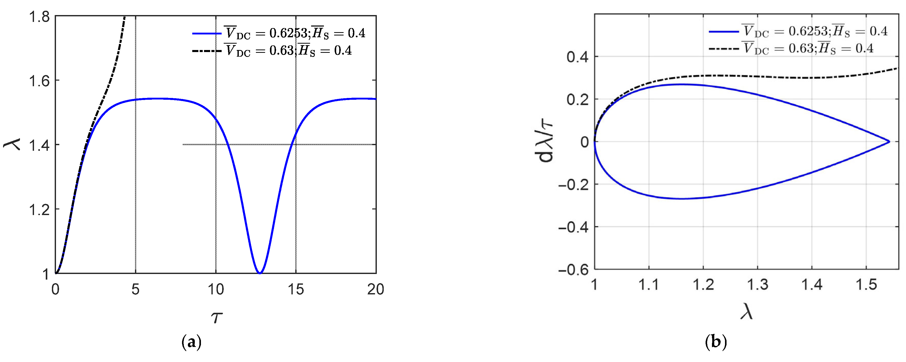
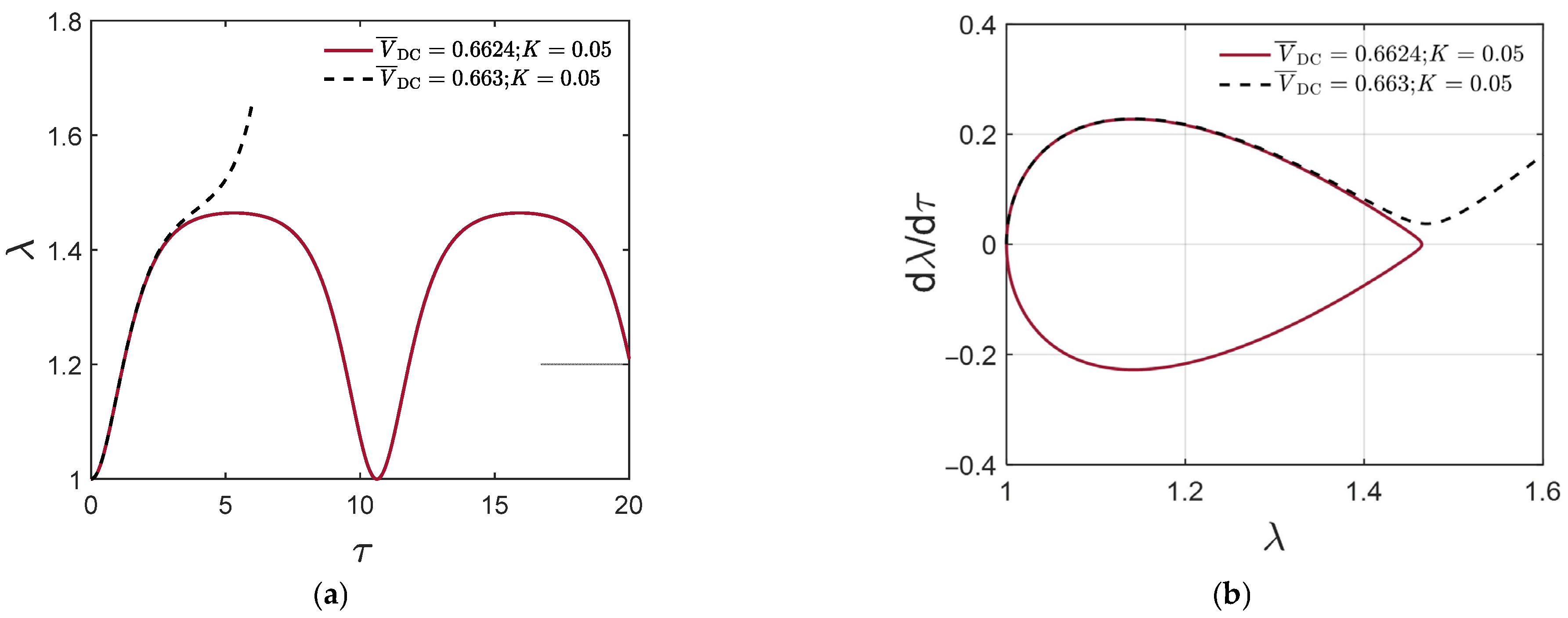
3.3. DC Dynamic Instability

First, the DC dynamic instability under the magneto-static field is analyzed in this sub-section. It is assumed that the active polymer is excited by a DC Heaviside step voltage signal for such instability. To evaluate the DC dynamic critical voltage V ¯ D C and dynamic critical stretch λ m a x = λ D C , the following conservation of energy relation should be satisfied [52]:
U ¯ t 1 + U ¯ K t 1 = U ¯ t 2 + U ¯ K t 2
in which U ¯ K is the dimensionless kinetic energy.
It is assumed that in the initial position t 1 , the stretch is equal to λ = λ p obtained from Equation (19), and the velocity is zero, in such a way that U ¯ K t 1 = 0 . In t 2 , the velocity is equal to zero, and the stretch is λ = λ m a x . Thus, we can write:
  D ¯ = U ¯ t 2 U ¯ t 1 = 2 S 1 + λ m a x + H ¯ 2 2 λ m a x V 2 λ m a x 4 2 + 1 3 K 2 λ m a x 2 + λ m a x 4 + 2 S 1 + λ p H ¯ 2 2 λ p 4 H ¯ 2 2 λ p 4 H ¯ 2 2 λ p 4 + V ¯ 2 λ p 4 2 1 3 K 2 λ p 2 + λ p 4 1 2 J m Ln 1 3 + 1 λ m a x 4 + 2 λ m a x 2 J m + 1 2 J m Ln 1 3 + 1 λ p 4 + 2 λ p 2 J m = 0
To find the DC dynamic instability, we should set D ¯ / λ m a x = 0 and simultaneously solve it together with Equation (24), from which V ¯ D C and λ m a x = λ D C are deduced. Table 3 provides the results for V ¯ D C and λ m a x for different system parameters. Comparing Table 2 and Table 3, it is observed that the dynamic critical voltage is less than the static critical voltage.
Now, the results of the analytical study presented in Table 3 are also validated numerically. Numerical integration is conducted on Equation (18) to analyze the DC dynamic instability when the voltage, mechanical load, and magnetic field are static, i.e., V ¯ = V ¯ DC , H ¯ = H ¯ S , and S ¯ = S ¯ S . As test cases, the influence of the magnetic field and the second invariant are studied. The results are presented in a λ τ diagram (time history) and d λ / d τ λ diagram (phase plane). The fixed parameters are J m = 100 and S ¯ = S ¯ S = 0 , and the initial conditions are λ t = 0 = λ p and λ ˙ t = 0 = 0 .
The response of the system under H ¯ = H ¯ S = 0 and K = 0 is analyzed under two values of the DC voltage (i.e., V ¯ DC = 0.6494   &   0.65 ) and presented in Figure 2. Figure 2a shows the time history of the system under a DC dynamic condition, and Figure 2b is the plot of the phase plane diagram under such a condition. It is seen that when the static voltage is near the critical voltage obtained in Table 3, namely, V ¯ DC = 0.6494 , the response of the system is periodic. A slight increase in DC voltage, V ¯ DC = 0.65 , will result in the response becoming aperiodic, which is the emergence of the DC dynamic instability in the system. This trend is observed in time history, where the trajectory is predictable and regular for a period response. Moreover, the periodic response indicates a closed loop in the phase plane. For aperiodic behavior, the stretch evolves beyond the critical starch; λ m a x = 1.4743 is the beginning of the instability.
The time history and phase plane diagram when the magnetic field is increased to H ¯ = H ¯ S = 0.4 and K = 0 are depicted in Figure 3. The values of DC voltage are chosen, i.e., V ¯ DC = 0.6253   &   0.63 . Similar to Figure 2, when the voltage is beyond the threshold, V ¯ DC = 0.6253 , the vibration becomes aperiodic, in which the stretch evolves to an unstable region. Comparing Figure 2 and Figure 3, it is concluded that a lower value of voltage is required for the onset of instability when the membrane is subjected to an external magnetic field. The results also show that the critical DC stretch is increased to λ m a x = 1.5447 from λ m a x = 1.4743 under the application of the magnetic field.
As the physical meaning of the second invariant is complex, this parameter has been generally neglected in a majority of works on active polymers. Based on the work conducted by Horgan and Smayda [45], the first invariant refers to a measure representing the average over all possible orientations of three times the squared stretches of an infinitesimal line element, and the second invariant refers to the exact same definition but for the area element. Moreover, the third invariant stands for the influence of volume change. Figure 4 shows the effect of the second invariant (selected as K = 0.05 )   on the instability in the absence of the magnetic field, H ¯ = H ¯ S = 0 . The critical DC voltage is selected from Table 3. Comparing Figure 2 for K = 0 and Figure 4 for K = 0.05 , it is concluded that with the inclusion of the second invariant, a higher value of voltage is required to enter the instability region.

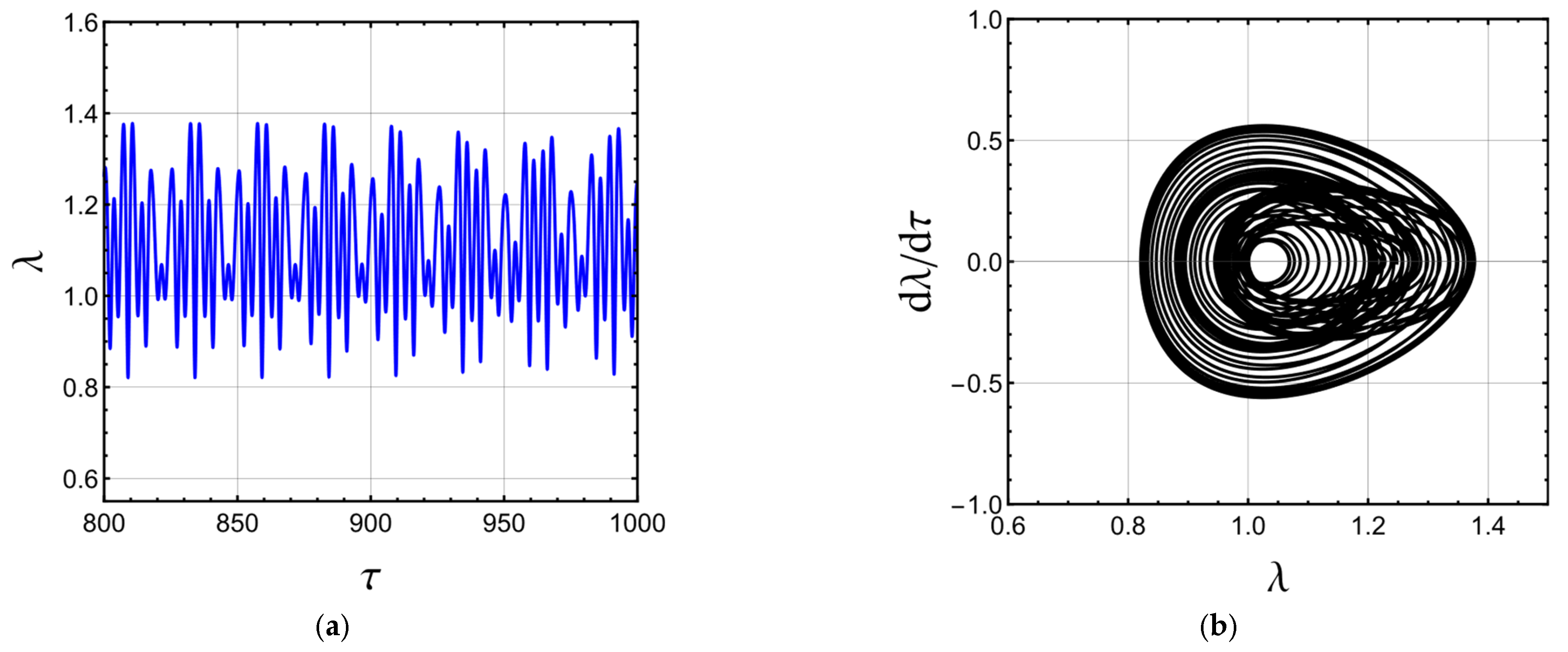
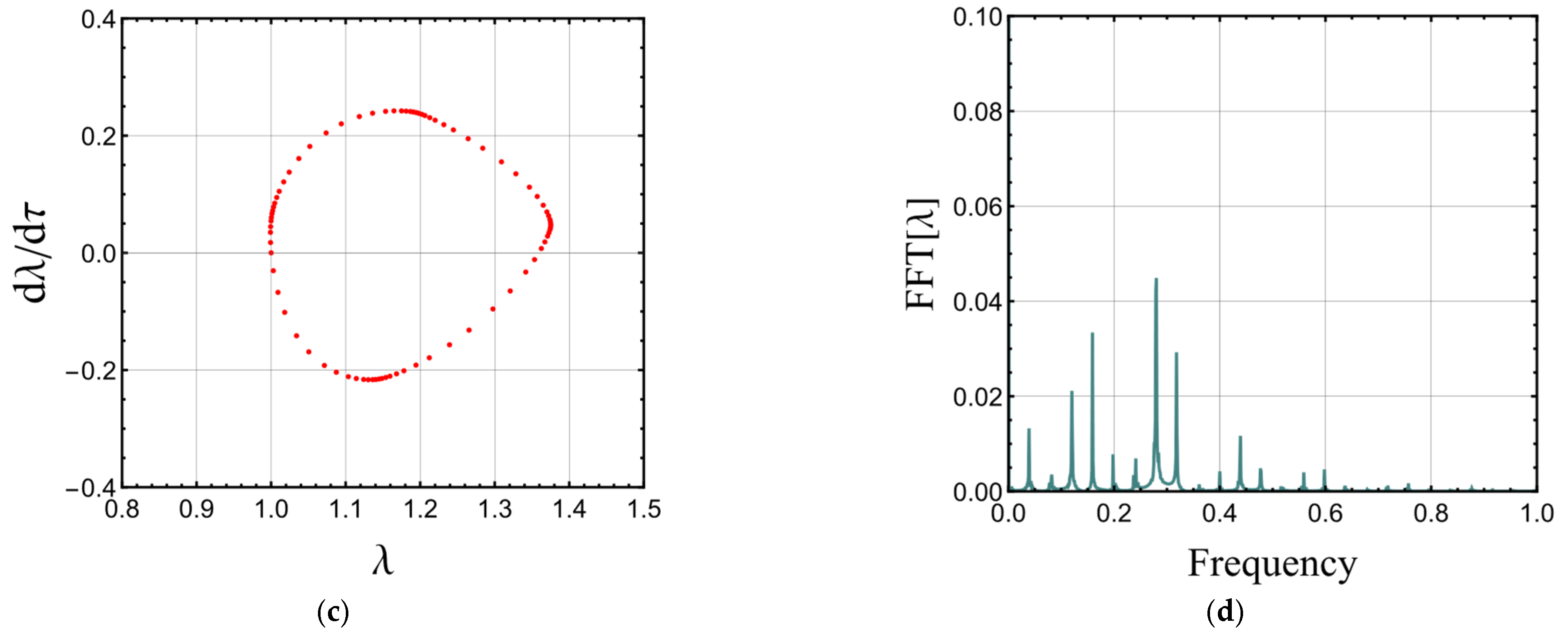
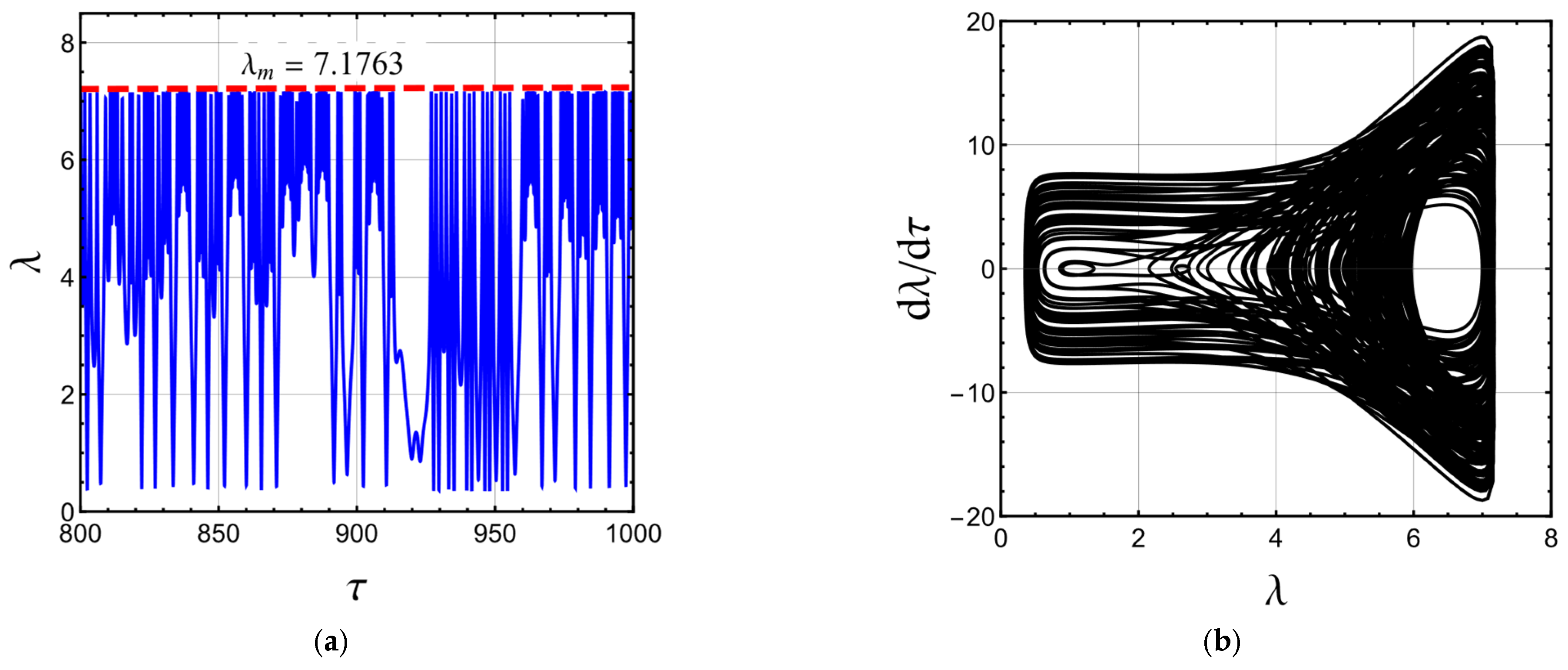
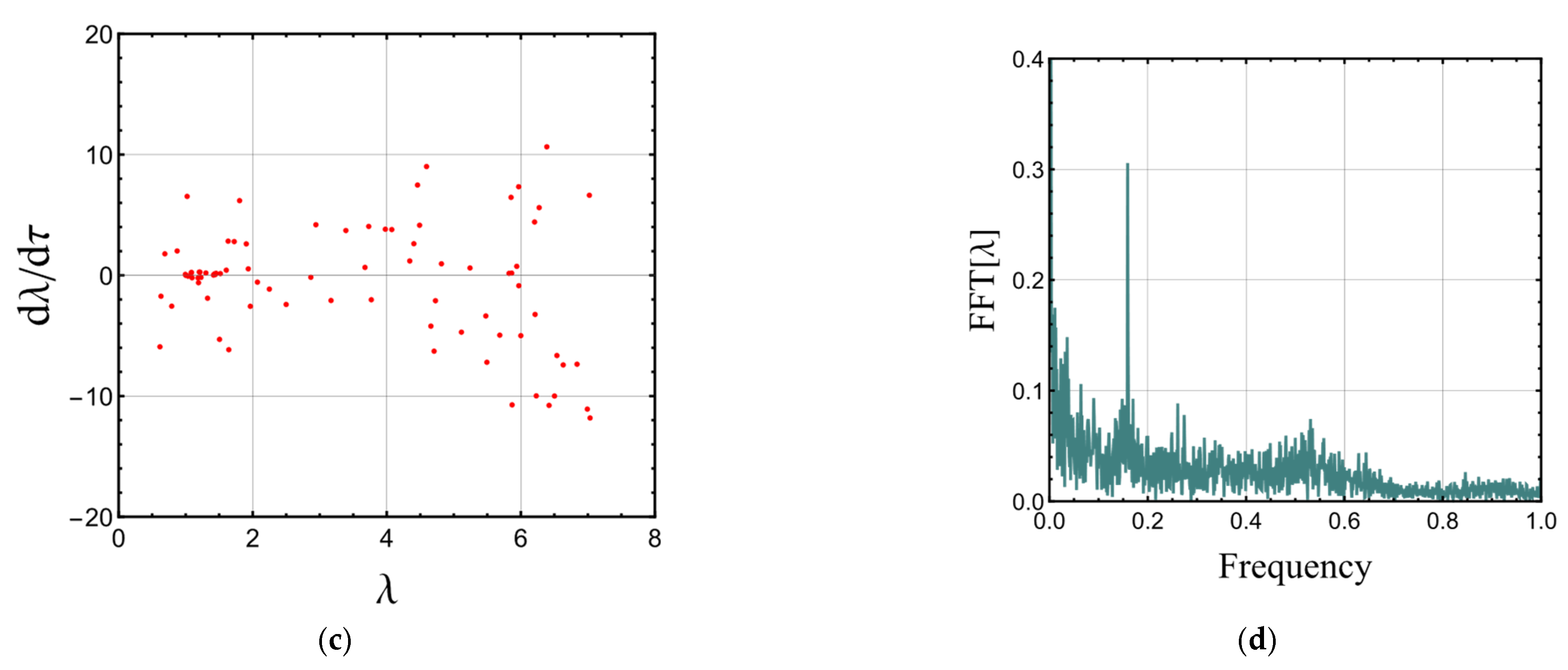
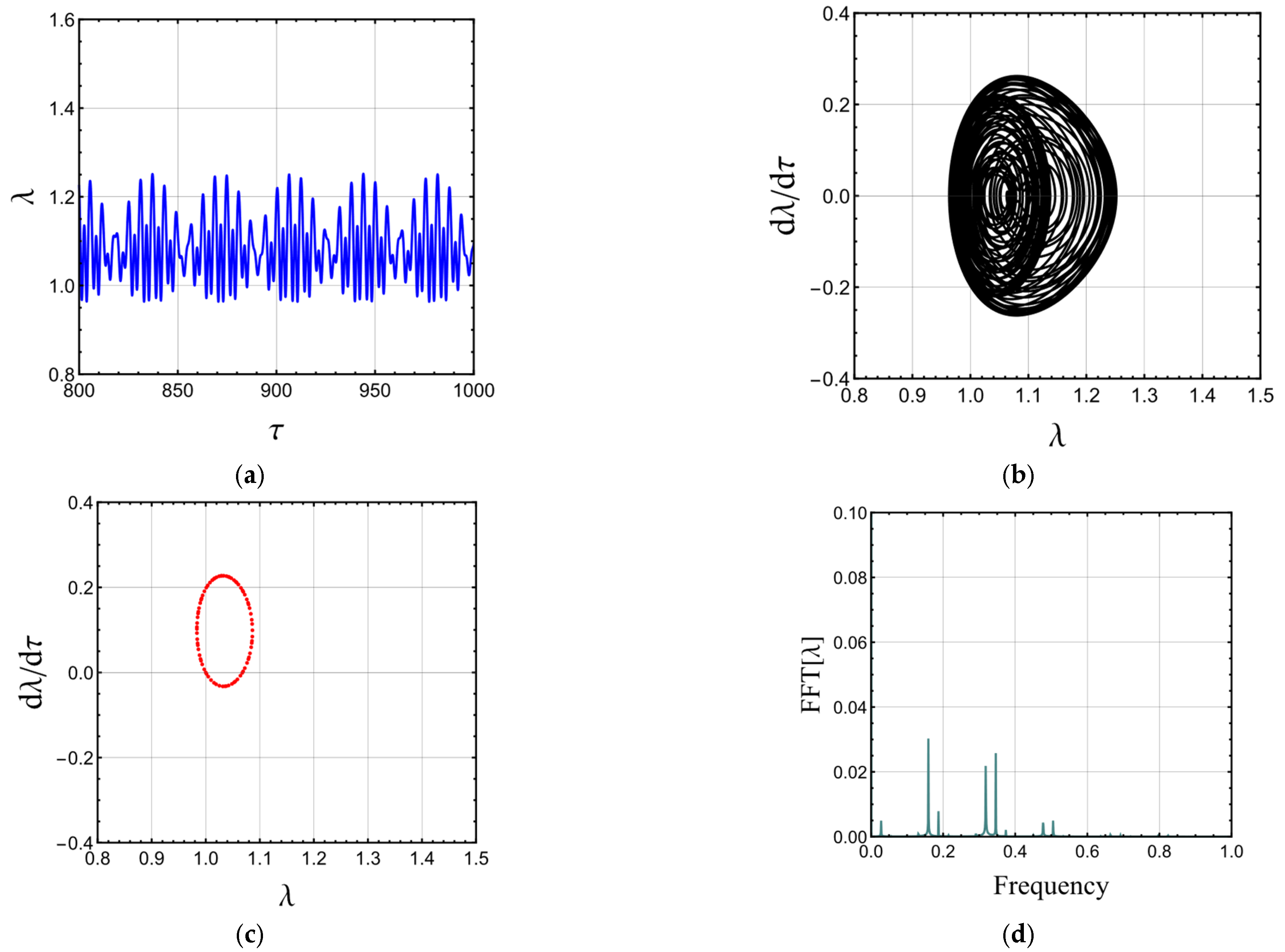
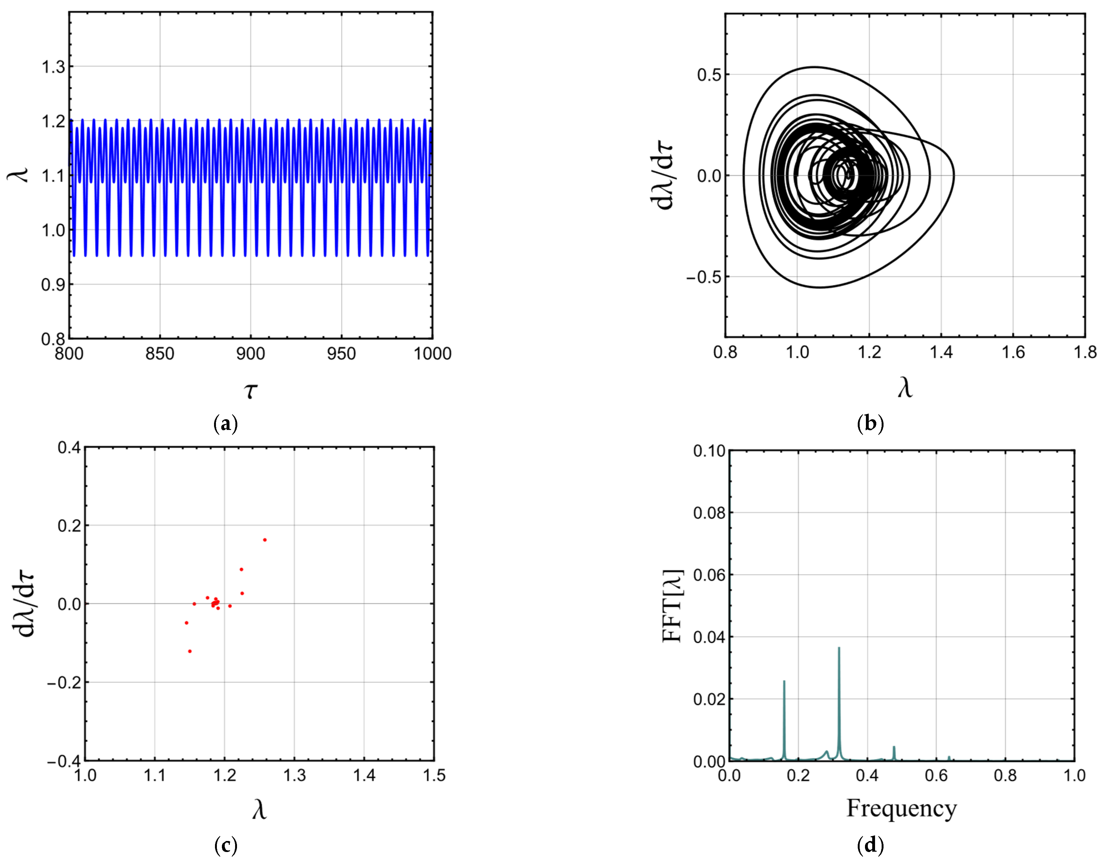
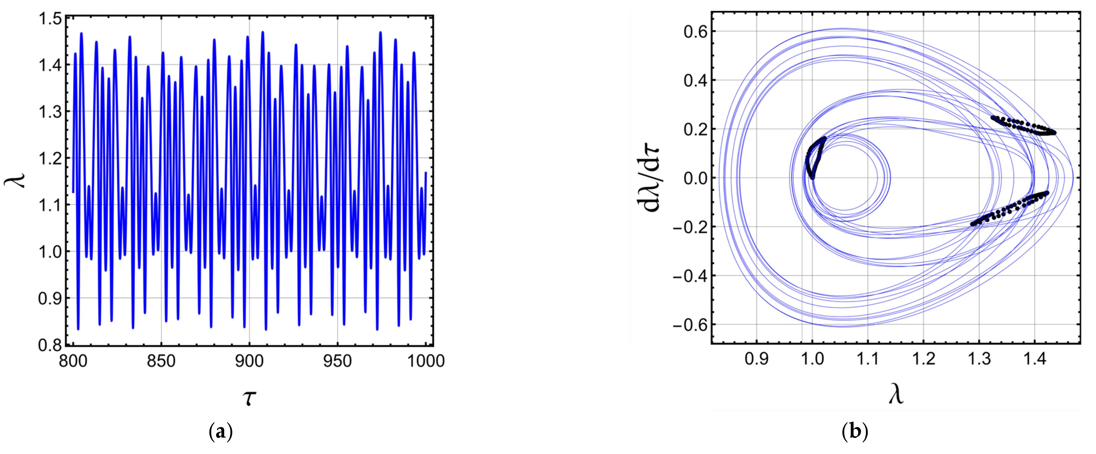
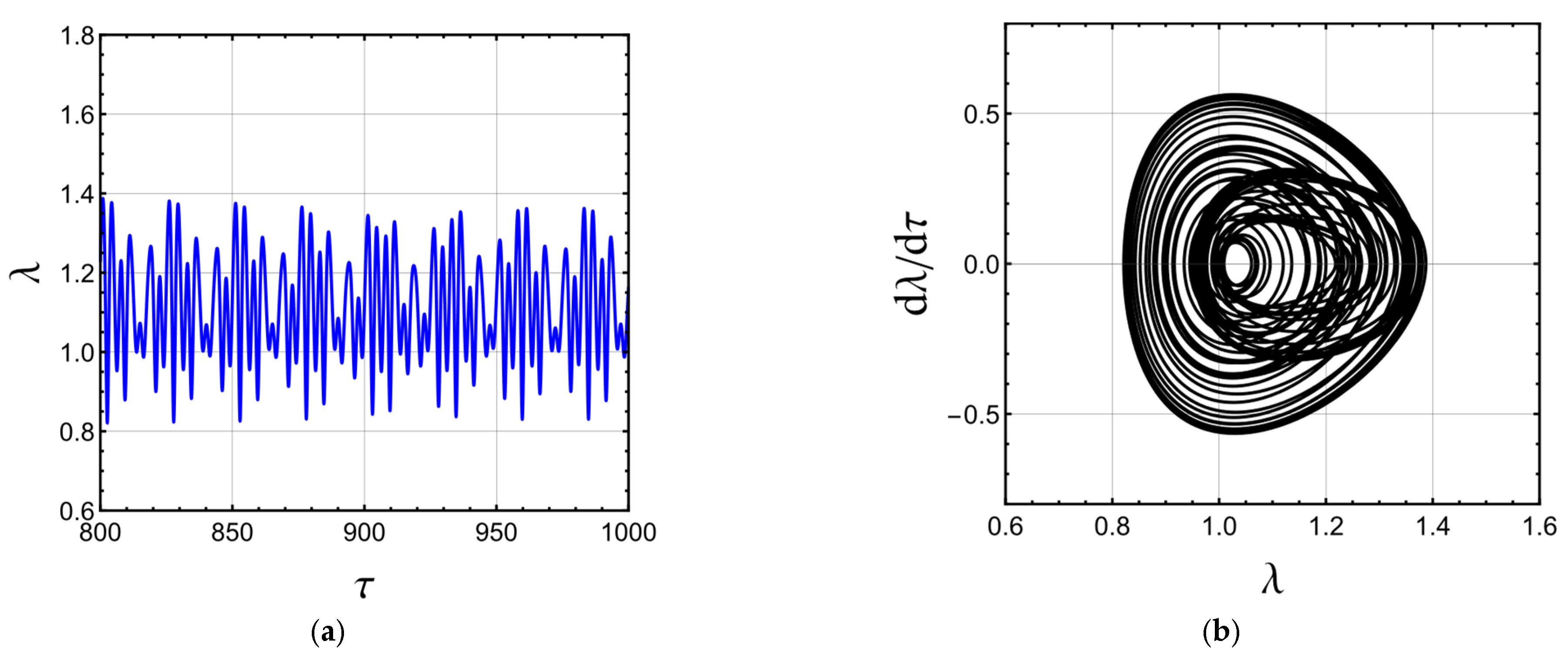
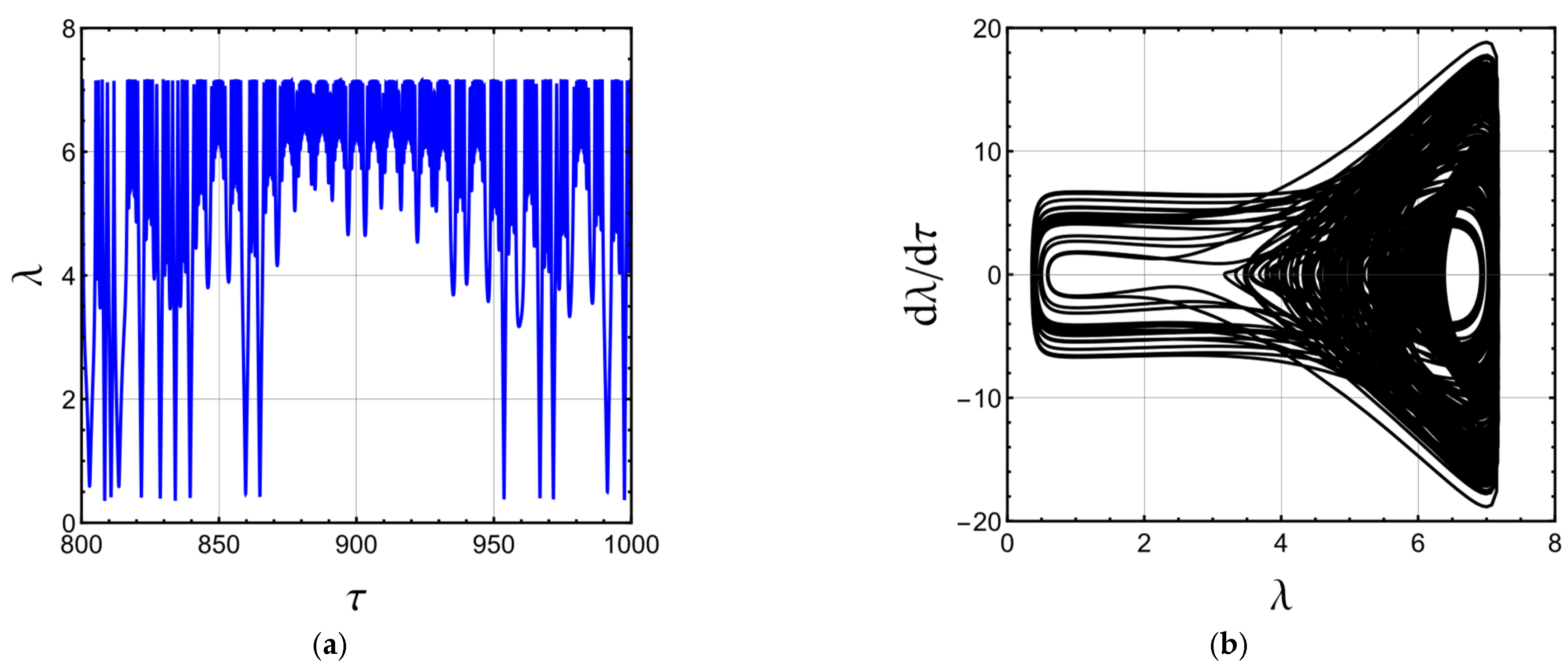
3.4. Dynamics under Time-Varying External Load

The previous sections focused on the static and DC dynamic instability of the system. In this section, the vibratory response of the MDE membrane shown in Figure 1 is investigated under time-varying external electrical and magnetic loads. Several cases have been investigated, and these include a time-varying voltage represented as:
V ¯ = V ¯ DC + V ¯ AC sin Ω t ,
augmented with a static magnetic force. In Equation (25), V ¯ AC stands for nondimensional AC voltage, and Ω = Ω 0 L ρ / 3 C 1 is the nondimensional excitation frequency ( Ω 0 is the original electrical excitation frequency).
Substituting Equation (25) into the governing dynamic equation, Equation (18), one can obtain:
λ ¨ + c λ ˙ + J m λ λ 5 J m 2 λ 2 λ 4 + 3 + 2 K λ 3 λ 3 2 λ 2 + λ 4 V ¯ DC 2 1 + V ¯ AC V ¯ DC sin Ω t 2 λ 3 H ¯ S 2 λ 5 S ¯ S = 0
It is noted that the time-dependent magnetic field is represented as:
H ¯ = H ¯ S + H ¯ D sin ω t ,
where H ¯ D represents the dynamic magnetic field, and ω = ω 0 L ρ / 3 C 1 is the nondimensional magnetic excitation frequency ( ω 0 is the original magnetic excitation frequency). Similarly, substituting Equation (27) into Equation (18) and considering static (DC) voltage yields:
λ ¨ + c λ ˙ + J m λ λ 5 J m 2 λ 2 λ 4 + 3 + 2 K λ 3 λ 3 2 λ 2 + λ 4 V ¯ DC 2 λ 3 H ¯ S 2 1 + H ¯ D H ¯ S sin ω t 2 λ 5 S ¯ S = 0
The effect of both the time-varying voltage and magnetic field, as given in Equations (25) and (27), are also investigated using the following relation:
λ ¨ + c λ ˙ + J m λ λ 5 J m 2 λ 2 λ 4 + 3 + 2 K λ 3 λ 3 2 λ 2 + λ 4 V ¯ DC 2 1 + V ¯ AC V ¯ DC sin Ω t 2 λ 3 H ¯ S 2 1 + H ¯ D H ¯ S sin ω t 2 λ 5 S ¯ S = 0
Hereafter, the dynamic of the system is analyzed when the system is actuated and subjected to the external loads described in the above cases. The numerical simulation is conducted by solving governing equations numerically using the Runge–Kutta method, and the results are depicted in different diagrams, for example, λ τ (time history), d λ / d τ λ (phase plane diagram), d λ / d τ λ (Poincaré map that is obtained by sampling at every period of the electrical load), and fast Fourier transform (FFT).
The results for H ¯ = H ¯ S = 0 , K = 0 , S ¯ = S ¯ S = 0 , V ¯ DC = 0.5 , V ¯ AC V ¯ DC = 0.3 , Ω = 1 , c = 0 , and J m = 100 are shown in Figure 5. This figure contains four subfigures: the time history, phase plane diagram, Poincaré map, and fast Fourier transform (FFT). As it can be realized, the response is quasiperiodic when the membrane is only subjected to electrical load under the considered parameters. Quasiperiodicity is observable in the Poincaré map, where a closed loop arises.
The effect of varying the static magnetic field and parameters K , c ,   and J m on the dynamics of the MDE membrane under time-varying voltage is also investigated. For instance, Figure 6 presents results for H ¯ S = 0.4 , K = 0 , S ¯ = S ¯ S = 0 , V ¯ DC = 0.5 , V ¯ AC V ¯ DC = 0.3 , Ω = 1 , c = 0 , and J m = 100 . The results show that the applied static magnetic field H ¯ S substantially contributes to the vibration response of the MDE membrane. What stands out from Figure 6 is that with the increase in the static magnetic field H ¯ S from 0 to 0.4, the quasiperiodic oscillation is replaced by chaotic oscillation. Irregular and unpredictable trajectories are seen when the stretch evolves with time in Figure 6a, namely, time history; this trend shows the chaos in the system. Many points on the Poincaré map with an irregular shape are another symptom of chaotic behavior in the electro-magneto-active membrane. The phase plane diagram also exhibits irregularly closed and open loops, indicating a chaotic phenomenon. The chaotic vibration can also be seen in the FFT, where continuous and noisy spectra emerge, indicating a complicated, chaotic trend.
Figure 7 also shows the results for the active polymer under time-varying voltage, assuming H ¯ S = 0.4 , K = 0.3 , S ¯ S = 0 , V ¯ DC = 0.5 , V ¯ AC V ¯ DC = 0.3 , Ω = 1 , c = 0 , and J m = 100 . The aim is to investigate the influence of the second invariant integrated into parameter   K on the response of the MDE membrane under time-varying voltage and the presence of the static magnetic field. A comparison of Figure 6 and Figure 7 shows that with the inclusion of the second invariant, the response becomes quasiperiodic. This means that the second invariant can suppress the chaotic behavior caused by the applied static magnetic field, as shown in Figure 6.
The results for the case H ¯ S = 0.4 , K = 0 , S ¯ S = 0 , V ¯ DC = 0.5 , V ¯ AC V ¯ DC = 0.3 , Ω = 1 , c = 0.05 , and J m = 100 is presented in Figure 8. This figure evaluates the effect of damping on the vibratory response behavior of the MDE membrane under time-varying voltage and a static magnetic field. The results show that if the membrane is not ideal and possesses viscoelasticity with c = 0.05 , the chaotic motion induced by the static magnetic field in Figure 6 is suppressed. The evidence of nonchaotic motion in Figure 8 is that when the stretch changes with time, the trajectory becomes regular, and points in the Poincaré map evolve into a stable region with periodic n -motion after neglecting the transient response.
Figure 9 also shows the effect of changes in the parameter J m for H ¯ S = 0.4 , K = 0 , S ¯ S = 0 , V ¯ DC = 0.5 , V ¯ AC V ¯ DC = 0.3 , Ω = 1 , c = 0 , and J m = 40 . It is observed that for the membrane with strong strain stiffening of J m = 40 , in comparison to Figure 6, the response changes to quasiperiodic. As shown in Figure 6, the Poincaré map generated inside the phase plane (black dots) contains closed loops, which is a sign of quasiperiodicity.
The vibration response of the MDE membrane under the simultaneous application of time-varying voltage and a magnetic field assuming H ¯ S = 0.1 , K = 0 , S ¯ S = 0 , V ¯ DC = 0.5 , V ¯ AC V ¯ DC = 0.3 , Ω = 1 , c = 0 , J m = 100 ., H ¯ D H ¯ S = 0.1 , and ω = 1.5 are shown in Figure 10. As it can be realized, the system can undergo a stable quasiperiodic motion even with a coupled time-dependent external loading. Closed loops in the phase plane diagram are the advent of the quasiperiodic in Figure 10. However, as depicted in Figure 11, as the amplitude of the time-varying magnetic field is increased to H ¯ D H ¯ S = 0.5 from H ¯ D H ¯ S = 0.1 , chaotic behavior appears in the system. The results confirm the importance of the magnitude of the magnetic load. It is interesting to note that with the same loading condition considered in Figure 11, while the time-dependent voltage is neglected V ¯ AC V ¯ DC = 0 , the response reverts to quasiperiodicity similar to Figure 10.

4. Conclusions

This paper investigates the nonlinear vibration behaviors of the magnetodielectric effect in magnetorheological elastomers using an energy-based method, the Lagrangian equation, and the Runge–Kutta time integration algorithm. The elastomer was modeled using the Gent–Gent model, and the damping effect was also captured. Time histories, phase plane diagrams, Poincaré sections, and fast Fourier transform were utilized to distinguish between the system’s periodic, quasiperiodic, and chaotic motion. This paper concludes that:
  • The magneto-electro-active polymer may undergo quasiperiodic and chaotic motions.
  • Increasing the static magnetic field leads to chaos when the electric field is time-dependent.
  • The second invariant can suppress the influence of the static magnetic field.
  • The damping force can also overcome chaotic motion due to the increased static magnetic field.
  • Chaotic motion due to the increased static magnetic field can be suppressed by increasing the strain stiffening effect (decreasing the Gent parameter-limiting stretch).
  • With the inclusion of the static magnetic field, a smaller amount of static voltage is required for the onset of static and DC dynamic instabilities.
Due to the lack of data on the nonlinear dynamic analysis of magnetodielectric effects in magnetorheological elastomers, the results presented in this study can provide essential guidance on the design of high-performance dielectric elastomers used in producing linear motion with sound generation or in self-sensing actuators. This paper focused on simple geometry, but the electromagnetic excitations can be developed for other geometries of MDEs. More specifically, for MDE-based microbeams that are used in resonators and tunable microwave filters, the voltage and magnetic field excitations can improve their performance; therefore, it would be crucial to study such structures. In other words, the results of this paper can not only be extended to MDE-based magnetic sensors and transducers but also to different geometries and nanocomposites.

Author Contributions

Conceptualization, H.J. and R.S.; methodology, H.J.; software, H.J.; validation, H.J.; formal analysis, H.J.; investigation, H.J.; resources, H.J.; data curation, H.J.; writing—original draft preparation, H.J.; writing—review and editing, H.J. and R.S.; visualization, H.J.; supervision, R.S.; funding acquisition, R.S. All authors have read and agreed to the published version of the manuscript.

Funding

Funding (under grant No. RGPIN-2021-03482 and DGDND-2021-03482) from the Natural Sciences and Engineering Research Council of Canada (NSERC) is gratefully acknowledged.

Institutional Review Board Statement

Not applicable.

Data Availability Statement

Data will be available upon request.

Conflicts of Interest

The authors declare no conflict of interest.

References

  1. Kim, K.J.; Tadokoro, S. Electroactive Polymers for Robotic Applications: Artificial Muscles and Sensors; Springer: London, UK, 2007. [Google Scholar]
  2. Suo, Z. Theory of Dielectric Elastomers. Acta Mech. Solida Sin. 2010, 23, 549–578. [Google Scholar] [CrossRef]
  3. Yu, K.; Xin, A.; Wang, Q. Mechanics of Light-Activated Self-Healing Polymer Networks. J. Mech. Phys. Solids 2019, 124, 643–662. [Google Scholar] [CrossRef]
  4. Alibakhshi, A.; Heidari, H. Nonlinear Resonance Analysis of Dielectric Elastomer Actuators under Thermal and Isothermal Conditions. Int. J. Appl. Mech. 2020, 12, 2050100. [Google Scholar] [CrossRef]
  5. Hamid Jafari, R.S. Analysis of an Adaptive Periodic Low-Frequency Wave Filter Featuring Magnetorheological Elastomers. Polymers 2023, 15, 735. [Google Scholar] [CrossRef]
  6. Jafari, H.; Ghodsi, A.; Azizi, S.; Ghazavi, M.R. Energy Harvesting Based on Magnetostriction, for Low-Frequency Excitations. Energy 2017, 124, 1–8. [Google Scholar] [CrossRef]
  7. Zuo, Y.; Ding, Y.; Zhang, J.; Zhu, M.; Liu, L.; Zhao, J. Humidity Effect on Dynamic Electromechanical Properties of Polyacrylic Dielectric Elastomer: An Experimental Study. Polymers 2021, 13, 784. [Google Scholar] [CrossRef]
  8. Hu, W.; Lum, G.Z.; Mastrangeli, M.; Sitti, M. Small-Scale Soft-Bodied Robot with Multimodal Locomotion. Nature 2018, 554, 81–85. [Google Scholar] [CrossRef]
  9. Jafari, H.; Ghodsi, A.; Ghazavi, M.R.; Azizi, S. Novel Mass Detection Based on Magnetic Excitation in Anti-Resonance Region. Microsyst. Technol. 2016, 23, 4–10. [Google Scholar] [CrossRef]
  10. Isaev, D.; Semisalova, A.; Alekhina, Y.; Makarova, L.; Perov, N. Simulation of Magnetodielectric Effect in Magnetorheological Elastomers. Int. J. Mol. Sci. 2019, 20, 1457. [Google Scholar] [CrossRef] [Green Version]
  11. Semisalova, A.S.; Perov, N.S.; Stepanov, G.V.; Kramarenko, E.Y.; Khokhlov, A.R. Strong Magnetodielectric Effects in Magnetorheological Elastomers. Soft Matter 2013, 9, 11318–11324. [Google Scholar] [CrossRef]
  12. Martins, P.; Silva, D.; Silva, M.P.; Lanceros-Mendez, S. Improved Magnetodielectric Coefficient on Polymer Based Composites through Enhanced Indirect Magnetoelectric Coupling. Appl. Phys. Lett. 2016, 109, 112905. [Google Scholar] [CrossRef] [Green Version]
  13. Morales, C.; Dewdney, J.; Pal, S.; Skidmore, S.; Stojak, K.; Srikanth, H.; Weller, T.; Wang, J. Tunable Magneto-Dielectric Polymer Nanocomposites for Microwave Applications. IEEE Trans. Microw. Theory Tech. 2011, 59, 302–310. [Google Scholar] [CrossRef]
  14. Yang, T.I.; Brown, R.N.C.; Kempel, L.C.; Kofinas, P. Surfactant-Modified Nickel Zinc Iron Oxide/Polymer Nanocomposites for Radio Frequency Applications. J. Nanoparticle Res. 2010, 12, 2967–2978. [Google Scholar] [CrossRef]
  15. Castro, J.; Morales, C.; Weller, T.; Wang, J.; Srikanth, H. Synthesis and Characterization of Low-Loss Fe3O4-PDMS Magneto-Dielectric Polymer Nanocomposites for RF Applications. In Proceedings of the WAMICON 2014, Tampa, FL, USA, 6 June 2014; pp. 1–5. [Google Scholar]
  16. Mitra, S.; Mondal, O.; Saha, D.R.; Datta, A.; Banerjee, S.; Chakravorty, D. Magnetodielectric Effect in Graphene-PVA Nanocomposites. J. Phys. Chem. C 2011, 115, 14285–14289. [Google Scholar] [CrossRef] [Green Version]
  17. Yang, T.I.; Brown, R.N.C.; Kempel, L.C.; Kofinas, P. Magneto-Dielectric Properties of Polymer- Fe3O4 Nanocomposites. J. Magn. Magn. Mater. 2008, 320, 2714–2720. [Google Scholar] [CrossRef]
  18. O’Halloran, A.; O’Malley, F.; McHugh, P. A Review on Dielectric Elastomer Actuators, Technology, Applications, and Challenges. J. Appl. Phys. 2008, 104, 071101. [Google Scholar] [CrossRef]
  19. Lu, T.; Ma, C.; Wang, T. Mechanics of Dielectric Elastomer Structures: A Review. Extrem. Mech. Lett. 2020, 38, 100752. [Google Scholar] [CrossRef]
  20. Zhu, J.; Cai, S.; Suo, Z. Nonlinear Oscillation of a Dielectric Elastomer Balloon. Polym. Int. 2010, 59, 378–383. [Google Scholar] [CrossRef]
  21. Sheng, J.; Chen, H.; Li, B.; Wang, Y. Nonlinear Dynamic Characteristics of a Dielectric Elastomer Membrane Undergoing In-Plane Deformation. Smart Mater. Struct. 2014, 23, 045010. [Google Scholar] [CrossRef]
  22. Wang, F.; Lu, T.; Wang, T.J. Nonlinear Vibration of Dielectric Elastomer Incorporating Strain Stiffening. Int. J. Solids Struct. 2016, 87, 70–80. [Google Scholar] [CrossRef]
  23. Alibakhshi, A.; Dastjerdi, S.; Akgöz, B.; Civalek, Ö. Parametric Vibration of a Dielectric Elastomer Microbeam Resonator Based on a Hyperelastic Cosserat Continuum Model. Compos. Struct. 2022, 287, 115386. [Google Scholar] [CrossRef]
  24. Alibakhshi, A.; Heidari, H. Nonlinear Dynamic Responses of Electrically Actuated Dielectric Elastomer-Based Microbeam Resonators. J. Intell. Mater. Syst. Struct. 2021, 33, 558–571. [Google Scholar] [CrossRef]
  25. Allahyari, E.; Asgari, M. Nonlinear Dynamic Analysis of Anisotropic Fiber-Reinforced Dielectric Elastomers: A Mathematical Approach. J. Intell. Mater. Syst. Struct. 2021, 32, 2300–2324. [Google Scholar] [CrossRef]
  26. Allahyari, E.; Asgari, M. Effect of Fibers Configuration on Nonlinear Vibration of Anisotropic Dielectric Elastomer Membrane. Int. J. Appl. Mech. 2020, 12, 2050114. [Google Scholar] [CrossRef]
  27. Alibakhshi, A.; Jafari, H.; Rostam-alilou, A.; Bodaghi, M.; Sedaghati, R. Nonlinear Vibration Behaviors of Dielectric Elastomer Membranes under Multi-Frequency Excitations. Sens. Actuators A. Phys. 2023, 351, 114171. [Google Scholar] [CrossRef]
  28. Belyaeva, I.A.; Kramarenko, E.Y.; Stepanov, G.V.; Sorokin, V.V.; Stadler, D.; Shamonin, M. Transient Magnetorheological Response of Magnetoactive Elastomers to Step and Pyramid Excitations. Soft Matter 2016, 12, 2901–2913. [Google Scholar] [CrossRef]
  29. Borin, D.Y.; Stepanov, G. V Elastomer with Magneto-and Electrorheological Properties. J. Intell. Mater. Syst. Struct. 2015, 26, 1893–1898. [Google Scholar] [CrossRef] [Green Version]
  30. Pelteret, J.P.; Steinmann, P. Magneto-Active Polymers: Fabrication, Characterisation, Modelling and Simulation at the Micro- and Macro-Scale; De Gruyter: Berlin, Germany, 2020; pp. 1–379. [Google Scholar] [CrossRef]
  31. Ghodsi, A.; Jafari, H.; Azizi, S.; Ghazavi, M.R. On the Dynamics of a Novel Energy Harvester to Convert the Energy of the Magnetic Noise into Electrical Power. Energy 2020, 207, 118268. [Google Scholar] [CrossRef]
  32. Jafari, H.; Sedaghati, R. Optimization of Band Gap Area in the Low-Frequency In-Plane Elastic/Acoustic Passive Adaptive Metamaterial. In Proceedings of the AIAA SCITECH 2023 Forum, National Harbor, MD, USA, 23–27 January 2023; p. 2123. [Google Scholar]
  33. Yarali, E.; Baniasadi, M.; Zolfagharian, A.; Chavoshi, M.; Arefi, F.; Hossain, M.; Bastola, A.; Ansari, M.; Foyouzat, A.; Dabbagh, A.; et al. Magneto-/Electro-responsive Polymers toward Manufacturing, Characterization, and Biomedical/Soft Robotic Applications. Appl. Mater. Today 2022, 26, 101306. [Google Scholar] [CrossRef]
  34. Abdalaziz, M.; Vatandoost, H.; Sedaghati, R.; Rakheja, S. Development and Experimental Characterization of a Large-Capacity Magnetorheological Damper with Annular-Radial Gap. Smart Mater. Struct. 2022, 31, 115021. [Google Scholar] [CrossRef]
  35. Montgomery, S.M.; Wu, S.; Kuang, X.; Armstrong, C.D.; Zemelka, C.; Ze, Q.; Zhang, R.; Zhao, R.; Qi, H.J. Magneto-Mechanical Metamaterials with Widely Tunable Mechanical Properties and Acoustic Bandgaps. Adv. Funct. Mater. 2021, 31, 1–10. [Google Scholar] [CrossRef]
  36. Kafle, A.; Luis, E.; Silwal, R.; Pan, H.M.; Shrestha, P.L.; Bastola, A.K. 3d/4d Printing of Polymers: Fused Deposition Modelling (Fdm), Selective Laser Sintering (Sls), and Stereolithography (Sla). Polymers 2021, 13, 3101. [Google Scholar] [CrossRef]
  37. Dorfmann, A.; Ogden, R.W. Nonlinear Magnetoelastic Deformations of Elastomers. Acta Mech. 2004, 167, 13–28. [Google Scholar] [CrossRef]
  38. Garcia-Gonzalez, D. Magneto-Visco-Hyperelasticity for Hard-Magnetic Soft Materials: Theory and Numerical Applications. Smart Mater. Struct. 2019, 28, 085020. [Google Scholar] [CrossRef]
  39. Zhao, R.; Kim, Y.; Chester, S.A.; Sharma, P.; Zhao, X. Mechanics of Hard-Magnetic Soft Materials. J. Mech. Phys. Solids 2019, 124, 244–263. [Google Scholar] [CrossRef]
  40. Khurana, A.; Kumar, D.; Sharma, A.K.; Joglekar, M.M. Static and Dynamic Instability Modeling of Electro-Magneto-Active Polymers with Various Entanglements and Crosslinks. Int. J. Non-Linear Mech. 2021, 139, 103865. [Google Scholar] [CrossRef]
  41. Haldar, K.; Kiefer, B.; Menzel, A. Finite Element Simulation of Rate-Dependent Magneto-Active Polymer Response. Smart Mater. Struct. 2016, 25, 104003. [Google Scholar] [CrossRef]
  42. Khurana, A.; Kumar, D.; Sharma, A.K.; Joglekar, M.M. Nonlinear Oscillations of Particle-Reinforced Electro-Magneto-Viscoelastomer Actuators. J. Appl. Mech. Trans. ASME 2021, 88, 1–19. [Google Scholar] [CrossRef]
  43. Xing, Z.; Yong, H. Dynamic Analysis and Active Control of Hard-Magnetic Soft Materials. Int. J. Smart Nano Mater. 2021, 12, 429–449. [Google Scholar] [CrossRef]
  44. Pucci, E.; Saccomandi, G. A Note on the Gent Model for Rubber-like Materials. Rubber Chem. Technol. 2002, 75, 839–852. [Google Scholar] [CrossRef]
  45. Horgan, C.O.; Smayda, M.G. The Importance of the Second Strain Invariant in the Constitutive Modeling of Elastomers and Soft Biomaterials. Mech. Mater. 2012, 51, 43–52. [Google Scholar] [CrossRef]
  46. Ogden, R.W.; Saccomandi, G.; Sgura, I. Fitting Hyperelastic Models to Experimental Data. Comput. Mech. 2004, 34, 484–502. [Google Scholar] [CrossRef] [Green Version]
  47. Khurana, A.; Kumar, A.; Raut, S.K.; Sharma, A.K.; Joglekar, M.M. Effect of Viscoelasticity on the Nonlinear Dynamic Behavior of Dielectric Elastomer Minimum Energy Structures. Int. J. Solids Struct. 2021, 208, 141–153. [Google Scholar] [CrossRef]
  48. Dutzler, A.; Buzzi, C.; Leitner, M. Nondimensional Translational Characteristics of Elastomer Components. J. Appl. Eng. Des. Simul. (JAEDS) 2021, 1, 18–24. [Google Scholar] [CrossRef]
  49. Lefèvre, V.; Lopez-Pamies, O. Nonlinear Electroelastic Deformations of Dielectric Elastomer Composites: I—Ideal Elastic Dielectrics. J. Mech. Phys. Solids 2017, 99, 409–437. [Google Scholar] [CrossRef] [Green Version]
  50. Nadzharyan, T.A.; Shamonin, M.; Kramarenko, E.Y. Theoretical Modeling of Magnetoactive Elastomers on Different Scales: A State-of-the-Art Review. Polymers 2022, 14, 4096. [Google Scholar] [CrossRef]
  51. Sharma, A.K.; Arora, N.; Joglekar, M.M. DC Dynamic Pull-in Instability of a Dielectric Elastomer Balloon: An Energy-Based Approach. Proc. R. Soc. A Math. Phys. Eng. Sci. 2018, 474, 20170900. [Google Scholar] [CrossRef] [Green Version]
  52. Alibakhshi, A.; Chen, W.; Destrade, M. Nonlinear Vibration and Stability of a Dielectric Elastomer Balloon Based on a Strain-Stiffening Model. J. Elast. 2022, 149, 1–16. [Google Scholar] [CrossRef]
Figure 1. The schematic of magneto/electroactive model (a) without external stimuli and (b) actuated with magnetic, electrical, and mechanical stimulants; Reference configuration in red X 1 , X 2 , X 3 ) and Actuated deformed configuration in black arrows x 1 , x 2 , x 3 .
Vibration 06 00017 g001
Figure 2. The DC dynamic response of the electro-magneto-active polymer to H ¯ = H ¯ S = 0 and   K = 0 . (a) Time history and (b) phase plane diagram.
Vibration 06 00017 g002
Figure 3. The DC dynamic response of the electro-magneto-active polymer to H ¯ = H ¯ S = 0.4 and   K = 0 . (a) Time history and (b) phase plane diagram.
Vibration 06 00017 g003
Figure 4. The DC dynamic response of the electro-magneto-active polymer to H ¯ = H ¯ S = 0 and   K = 0.05 . (a) Time history and (b) phase plane diagram.
Vibration 06 00017 g004
Figure 5. The dynamic response of the electro-magneto-active polymer to time-varying voltage H ¯ = H ¯ S = 0 . (a) Time history, (b) phase plane diagram, (c) Poincaré map, and (d) FFT.
Vibration 06 00017 g005aVibration 06 00017 g005b
Figure 6. The dynamic response of the electro-magneto-active polymer to time-varying voltage H ¯ = H ¯ S = 0.4 . (a) Time history, (b) phase plane diagram, (c) Poincaré map, and (d) FFT.
Vibration 06 00017 g006aVibration 06 00017 g006b
Figure 7. The dynamic response of the electro-magneto-active polymer to time-varying voltage H ¯ = H ¯ S = 0.4 and   K = 0.3 . (a) Time history, (b) phase plane diagram, (c) Poincaré map, and (d) FFT.
Vibration 06 00017 g007
Figure 8. The dynamic response of the electro-magneto-active polymer to time-varying voltage H ¯ = H ¯ S = 0.4 and   c = 0.05 . (a) Time history, (b) phase plane diagram, (c) Poincaré map, and (d) FFT.
Vibration 06 00017 g008
Figure 9. The dynamic response of the electro-magneto-active polymer to J m = 40 . (a) Time history and (b) phase plane diagram with Poincaré map inside it.
Vibration 06 00017 g009
Figure 10. The dynamic response of the electro-magneto-active polymer to H ¯ D H ¯ S = 0.1 . (a) Time history and (b) phase plane diagram.
Vibration 06 00017 g010
Figure 11. The dynamic response of the electro-magneto-active polymer to H ¯ D H ¯ S = 0.5 . (a) Time history and (b) phase plane diagram.
Vibration 06 00017 g011
Table 1. The initial stretch of the MAP subjected to mechanical load only.
S ¯ S K J m λ p
0 0 100 1
0 0.05 100 1
0 0 50 1
0.5 0.05 100 1.105382543
Table 2. The static critical voltage V ¯ D C C and static critical stretch λ s C .
S ¯ K J m H ¯ λ s C V ¯ pc C
0010001.26380.6893
0.5010001.43790.5164
00.0510001.26350.7036
001000.41.29580.6730
005001.26790.6914
Table 3. The static critical voltage V ¯ D C and static critical stretch λ m a x .
S ¯ K J m H ¯ λ max V ¯ pc c
0010001.47430.6494
0.5010001.70520.4889
00.0510001.47180.6624
001000.41.54470.6253
005001.48430.6521
Disclaimer/Publisher’s Note: The statements, opinions and data contained in all publications are solely those of the individual author(s) and contributor(s) and not of MDPI and/or the editor(s). MDPI and/or the editor(s) disclaim responsibility for any injury to people or property resulting from any ideas, methods, instructions or products referred to in the content.

