
An Evaluation of the Atmospheric Instability Effect on Wildfire Danger Using ERA5 over the Iberian Peninsula

 , , ,
, , , 
Abstract
:1. Introduction
2. Data and Methods
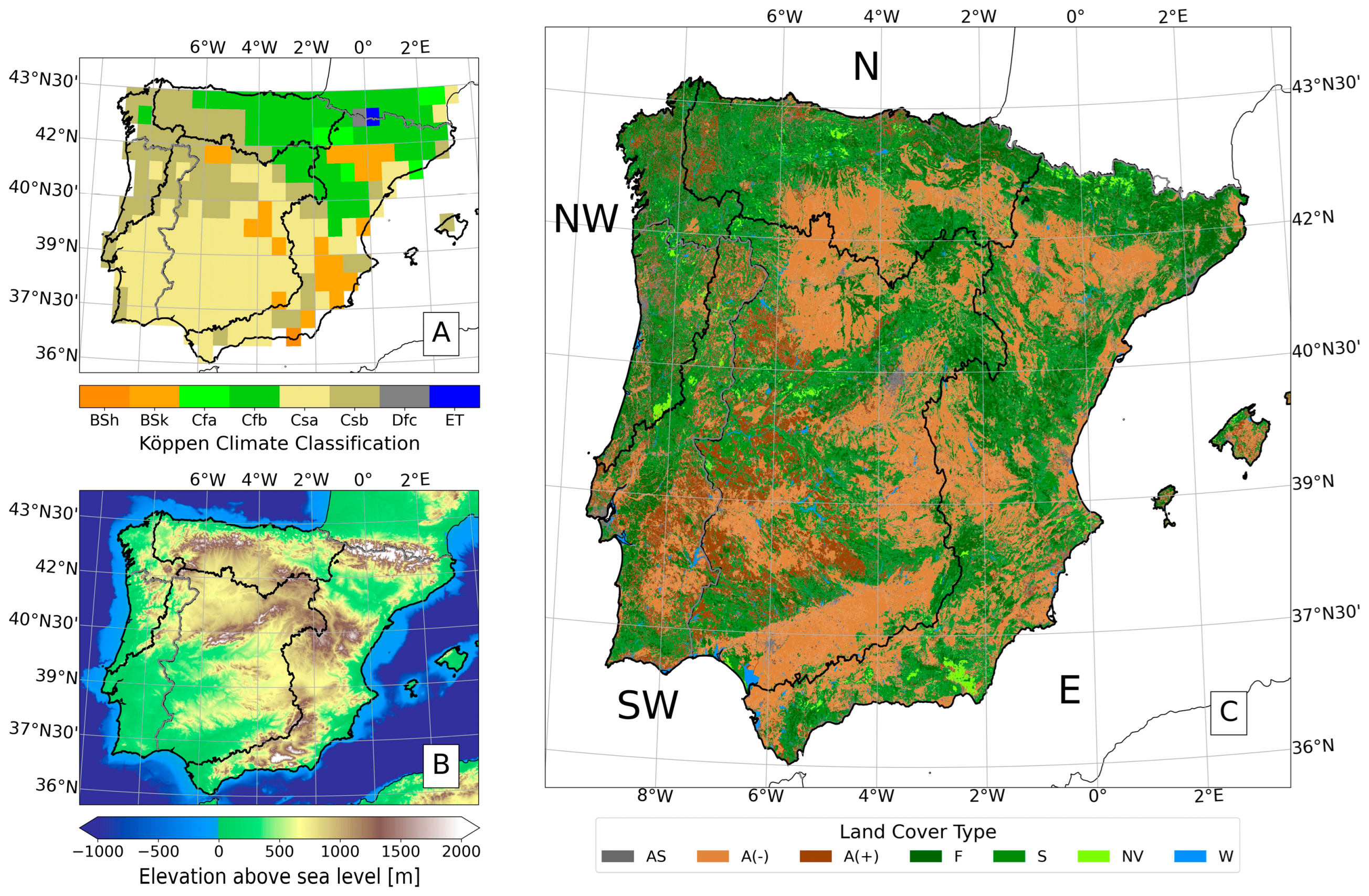
2.1. Study Region
2.2. Reanalysis Data
2.3. Continuous Haines Index
2.4. Fire Weather Index and Enhanced Fire Weather Index
2.5. Fire Radiative Power
2.6. Methods
3. Results
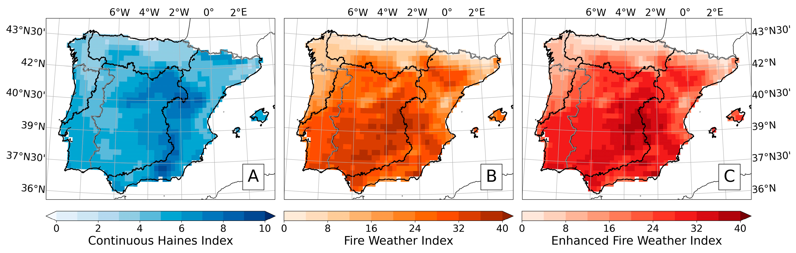
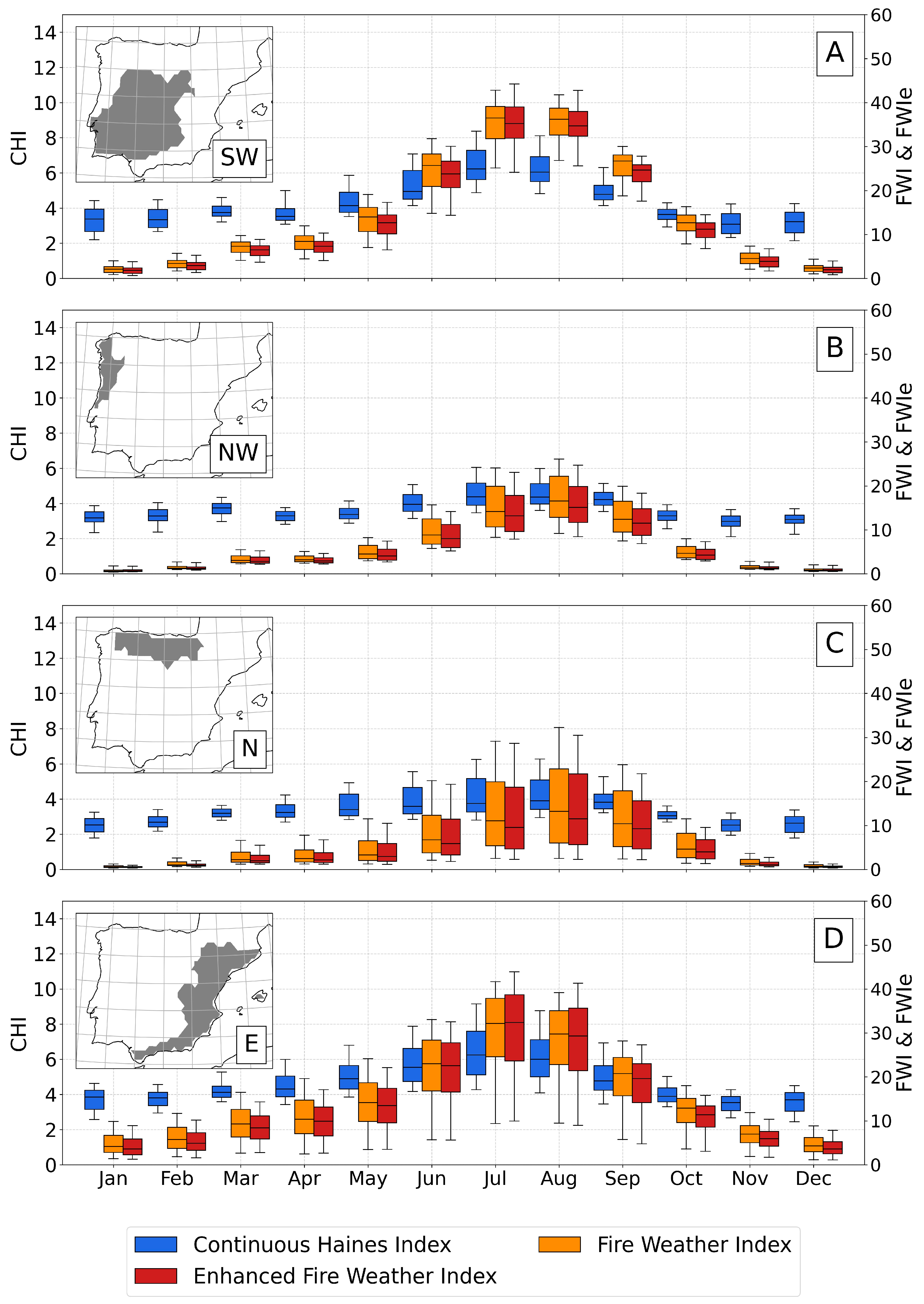
3.1. Climatological Analysis
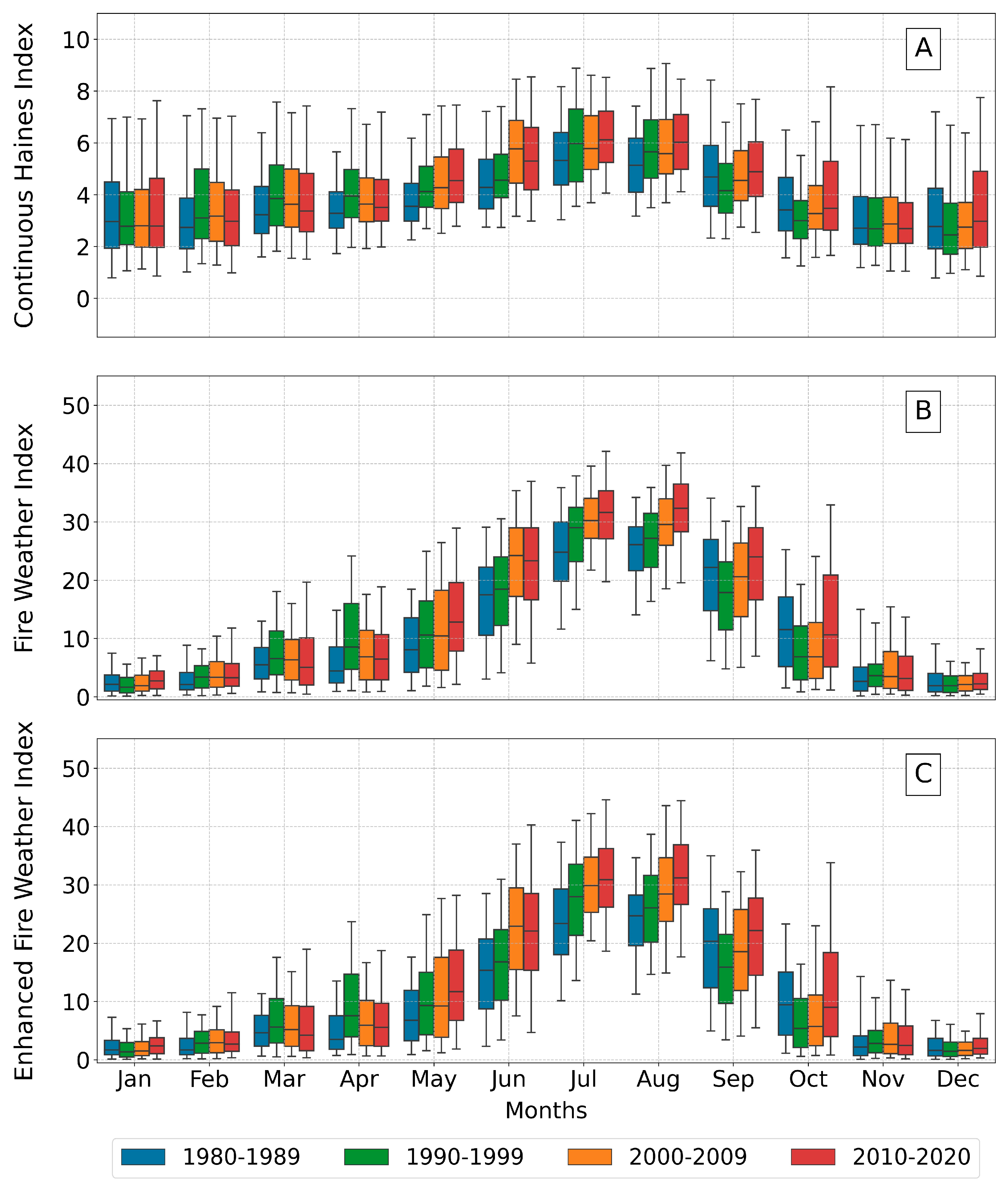
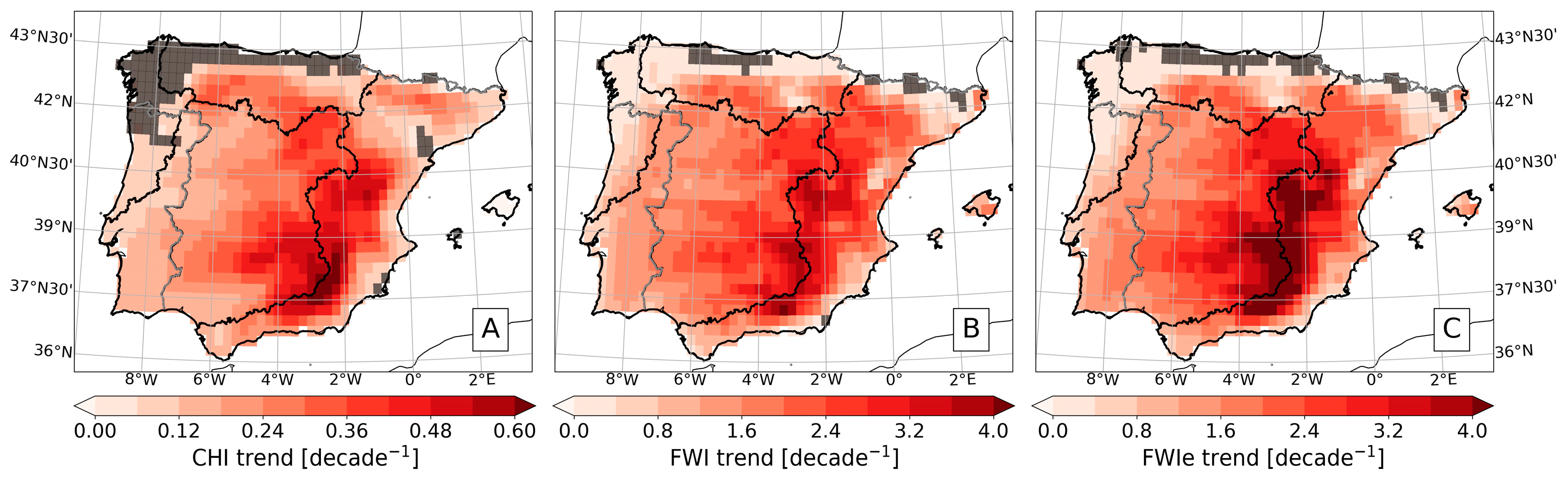
3.2. Decadal Evolution
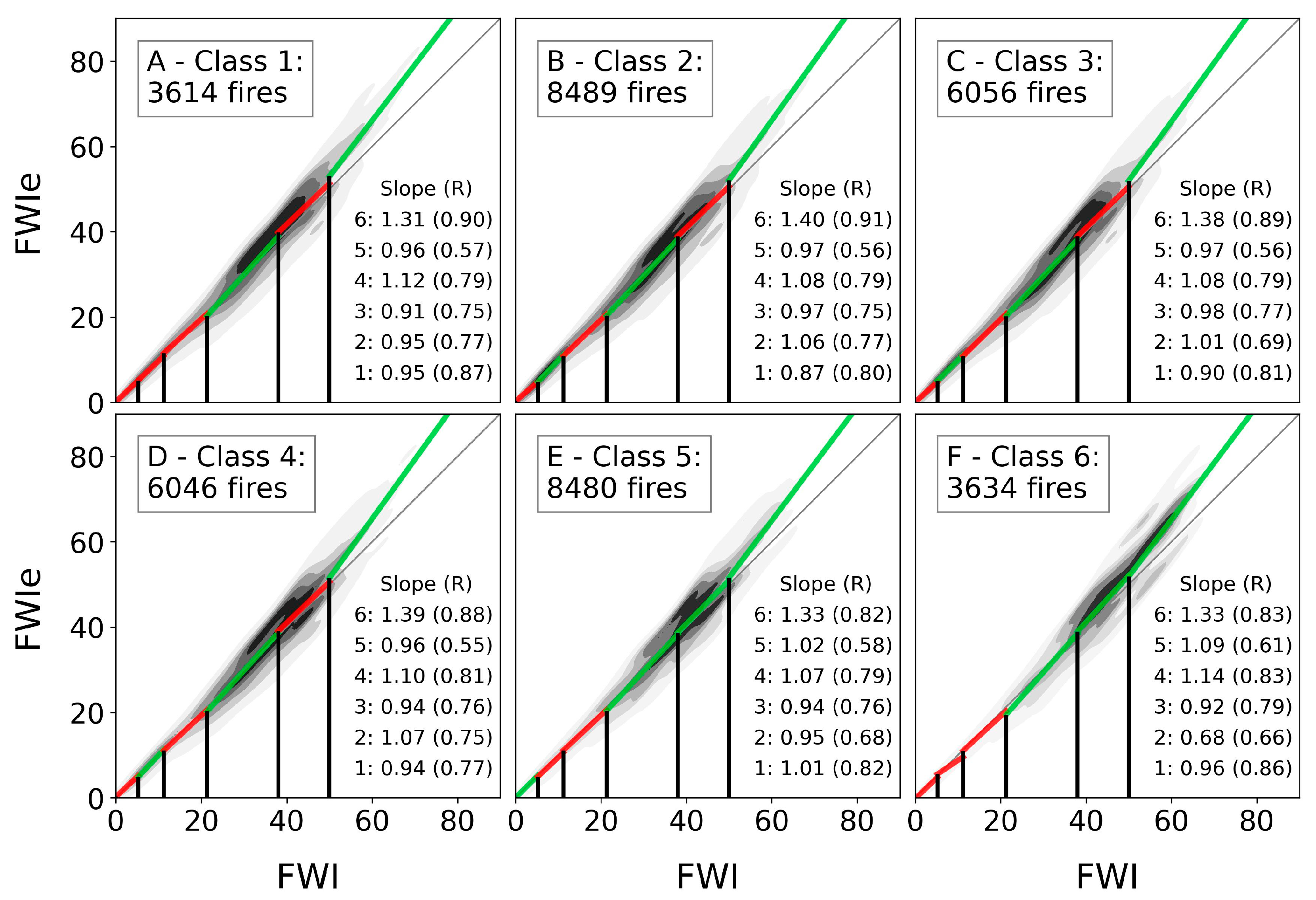
3.3. Fire Occurrences and FWI vs. FWIe
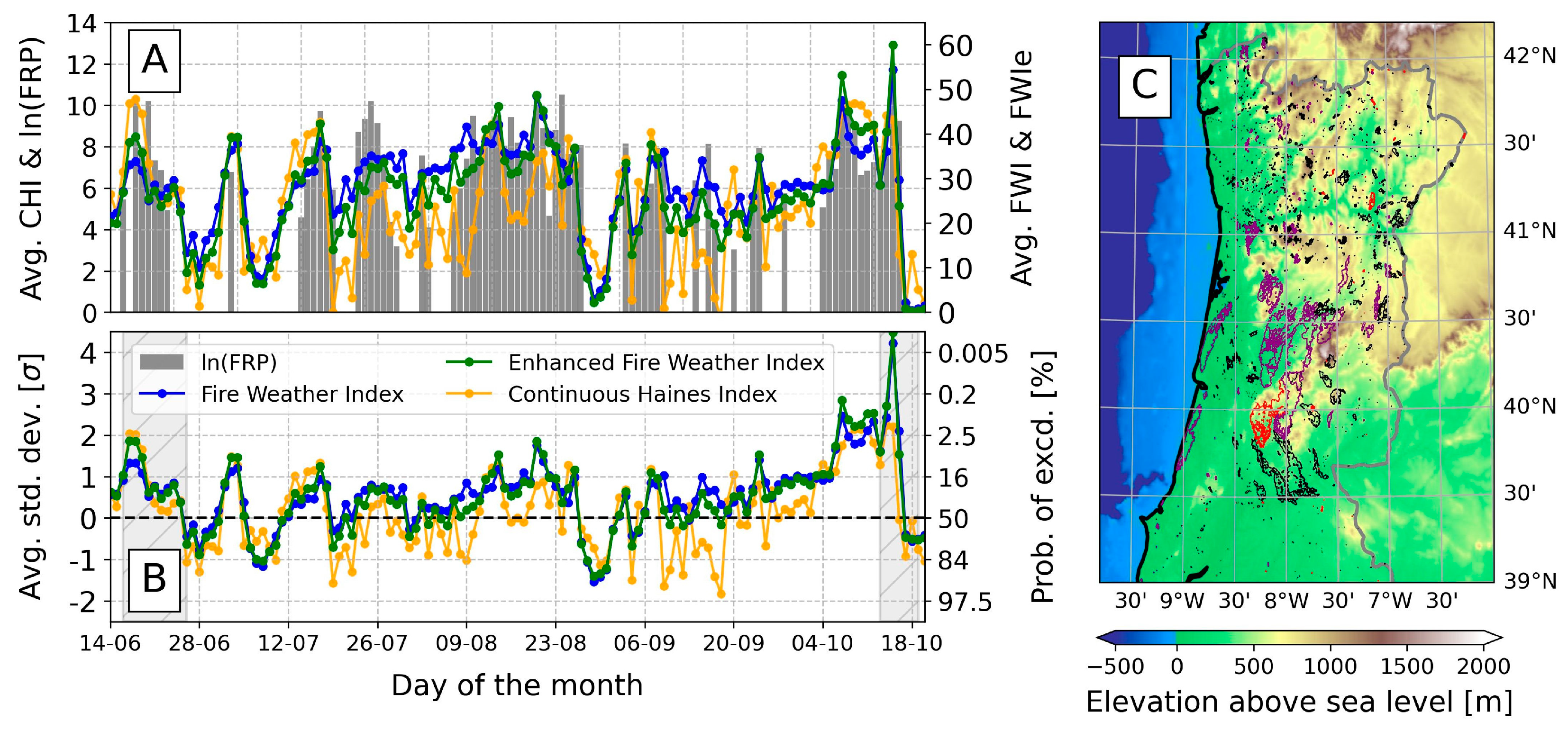
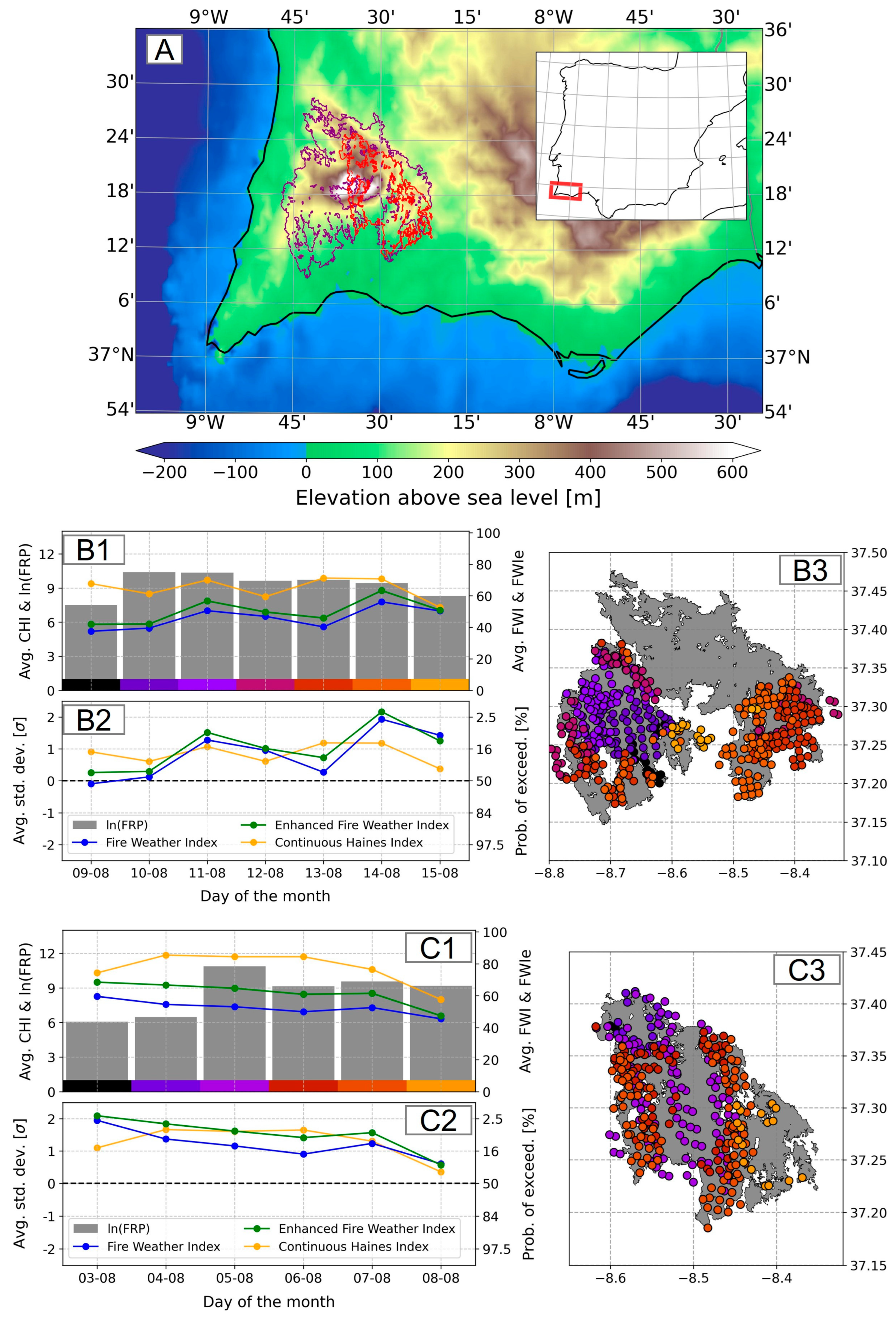
3.4. Case Studies
4. Discussion and Summary
5. Final Remarks
Supplementary Materials
Author Contributions
Funding
Institutional Review Board Statement
Informed Consent Statement
Data Availability Statement
Acknowledgments
Conflicts of Interest
References
- Amatulli, G.; Camia, A.; San-Miguel-Ayanz, J. Estimating future burned areas under changing climate in the EU-Mediterranean countries. Sci. Total Environ. 2013, 450, 209–222. [Google Scholar] [CrossRef] [PubMed]
- Amraoui, M.; Pereira, M.G.; DaCamara, C.C.; Calado, T.J. Atmospheric conditions associated with extreme fire activity in the Western Mediterranean region. Sci. Total Environ. 2015, 524, 32–39. [Google Scholar] [CrossRef] [PubMed]
- Fernandes, P.M.; Monteiro-Henriques, T.; Guiomar, N.; Loureiro, C.; Barros, A.M. Bottom-up variables govern large-fire size in Portugal. Ecosystems 2016, 19, 1362–1375. [Google Scholar] [CrossRef]
- Carmo, M.; Ferreira, J.; Mendes, M.; Silva, Á.; Silva, P.; Alves, D.; Reis, L.; Novo, I.; Viegas, D.X. The climatology of extreme wildfires in Portugal, 1980–2018: Contributions to forecasting and preparedness. Int. J. Climatol. 2021, 42, 3123–3146. [Google Scholar] [CrossRef]
- DaCamara, C.C.; Calado, T.J.; Ermida, S.L.; Trigo, I.F.; Amraoui, M.; Turkman, K.F. Calibration of the fire weather index over mediterranean europe based on fire activity retrieved from msg satellite imagery. Int. J. Wildland Fire 2014, 23, 945–958. [Google Scholar] [CrossRef]
- Trigo, R.M.; Pereira, J.M.; Pereira, M.G.; Mota, B.; Calado, T.J.; Dacamara, C.C.; Santo, F.E. Atmospheric conditions associated with the exceptional fire season of 2003 in Portugal. Int. J. Climatol. 2006, 26, 1741–1757. [Google Scholar] [CrossRef]
- Abatzoglou, J.T.; Williams, A.P.; Barbero, R. Global emergence of anthropogenic climate change in fire weather indices. Geophys. Res. Lett. 2019, 46, 326–336. [Google Scholar] [CrossRef] [Green Version]
- Bedia, J.; Herrera, S.; Camia, A.; Moreno, J.M.; Gutiérrez, J.M. Forest fire danger projections in the Mediterranean using ENSEMBLES regional climate change scenarios. Clim. Change 2014, 122, 185–199. [Google Scholar] [CrossRef] [Green Version]
- Calheiros, T.; Nunes, J.P.; Pereira, M.G. Recent evolution of spatial and temporal patterns of burnt areas and fire weather risk in the Iberian Peninsula. Agric. Forest Meteorol. 2020, 287, 107923. [Google Scholar] [CrossRef]
- Pereira, M.G.; Calado, T.J.; DaCamara, C.C.; Calheiros, T. Effects of regional climate change on rural fires in Portugal. Clim. Res. 2013, 57, 187–200. [Google Scholar] [CrossRef] [Green Version]
- Lionello, P.; Malanotte-Rizzoli, P.; Boscolo, R.; Alpert, P.; Artale, V.; Li, L.; Luterbacher, J.; May, W.; Trigo, R.; Tsimplis, M.; et al. The Mediterranean climate: An overview of the main characteristics and issues. Dev. Earth Environ. Sci. 2006, 4, 1–26. [Google Scholar] [CrossRef]
- Nunes, S.A.; DaCamara, C.C.; Turkman, K.F.; Calado, T.J.; Trigo, R.M.; Turkman, M.A. Wildland fire potential outlooks for Portugal using meteorological indices of fire danger. Nat. Hazard. Earth Sys. 2019, 19, 1459–1470. [Google Scholar] [CrossRef] [Green Version]
- San-Miguel-Ayanz, J.; Durrant, T.; Boca, R.; Maianti, P.; Libertá, G.; Artés Vivancos, T.; Jacome Felix Oom, D.; Branco, A.; De Rigo, D.; Ferrari, D.; et al. Forest Fires in Europe, Middle East and North Africa 2020; Publications Office of the European Union: Luxembourg, 2021. [Google Scholar] [CrossRef]
- Leone, V.; Lovreglio, R.; Martín, M.P.; Martínez, J.; Vilar, L. Human factors of fire occurrence in the Mediterranean. In Earth Observation of Wildland Fires in Mediterranean Ecosystems, 1st ed.; Springer: Berlin, Germany, 2009; pp. 149–170. [Google Scholar] [CrossRef]
- Gómez-González, S.; Ojeda, F.; Fernandes, P.M. Portugal and Chile: Longing for sustainable forestry while rising from the ashes. Environ. Sci. Policy 2018, 81, 104–107. [Google Scholar] [CrossRef]
- Alcubierre, P.C.; Ribau, M.C.; de Egileor, A.L.O.; Bover, M.M.; Kraus, P.D. Prevention of Large Wildfires Using the Fire Types Concept; Unitat Técnica del GRAF: Barcelona, Spain, 2011. [Google Scholar]
- Lecina-Diaz, J.; Alvarez, A.; Retana, J. Extreme fire severity patterns in topographic, convective and wind-driven historical wildfires of Mediterranean pine forests. PLoS ONE 2014, 9, e85127. [Google Scholar] [CrossRef] [PubMed] [Green Version]
- Pinto, M.M.; DaCamara, C.C.; Hurduc, A.; Trigo, R.M.; Trigo, I.F. Enhancing the fire weather index with atmospheric instability information. Environ. Res. Lett. 2020, 15, 0940b7. [Google Scholar] [CrossRef]
- Ruffault, J.; Moron, V.; Trigo, R.M.; Curt, T. Daily synoptic conditions associated with large fire occurrence in Mediterranean France: Evidence for a wind-driven fire regime. Int. J. Climatol. 2017, 37, 524–533. [Google Scholar] [CrossRef]
- Flatley, W.T.; Lafon, C.W.; Grissino-Mayer, H.D. Climatic and topographic controls on patterns of fire in the southern and central Appalachian Mountains, USA. Landsc. Ecol. 2011, 26, 195–209. [Google Scholar] [CrossRef]
- Lareau, N.P.; Clements, C.B. The mean and turbulent properties of a wildfire convective plume. J. Appl. Meteorol. Clim. 2017, 56, 2289–2299. [Google Scholar] [CrossRef] [Green Version]
- Jolly, W.M.; Freeborn, P.H.; Page, W.G.; Butler, B.W. Severe fire danger index: A forecastable metric to inform firefighter and community wildfire risk management. Fire J. 2019, 2, 47. [Google Scholar] [CrossRef] [Green Version]
- Van Wagner, C. Development and Structure of the Canadian Forest Fire Weather Index System; Can. For. Serv., Forestry Tech. Rep.: Ottawa, Canada, 1987. [Google Scholar]
- Karali, A.; Roussos, A.; Giannakopoulos, C.; Hatzaki, M.; Xanthopoulos, G.; Kaoukis, K. Evaluation of the Canadian Fire Weather Index in Greece and future climate projections. In Advances in Meteorology; Springer: Berlin/Heidelberg, Germany, 2013; pp. 501–508. [Google Scholar] [CrossRef]
- Pinto, M.M.; DaCamara, C.C.; Trigo, I.F.; Trigo, R.M.; Turkman, K.F. Fire danger rating over mediterranean europe based on fire radiative power derived from meteosat. Nat. Hazard Earth Sys. 2018, 18, 515–529. [Google Scholar] [CrossRef] [Green Version]
- Wang, Y.; Anderson, K.R.; Suddaby, R.M. Updated source code for calculating fire danger indices in the Canadian Forest Fire Weather Index System. In Canadian Forest Service, Northern Forestry Centre Information Rep, Natural Resources Canada; NOR-X-424: Edmonton, Canada, 2015; p. 26. Available online: https://cfs.nrcan.gc.ca/publications (accessed on 11 March 2022).
- Haines, D.A. A lower atmospheric severity index for wildland fires. Natl. Weather. Dig. 1988, 13, 23–27. [Google Scholar]
- Dowdy, A.J.; Pepler, A. Pyroconvection risk in Australia: Climatological changes in atmospheric stability and surface fire weather conditions. Geophys. Res. Lett. 2018, 45, 2005–2013. [Google Scholar] [CrossRef]
- Mills, G.A.; McCaw, L. Atmospheric Stability Environments and Fire Weather in Australia—Extending the Haines Index; Technical Report; Centre for Australian Weather and Climate Research: Victoria, Australia, 2010; Volume 20. [Google Scholar]
- Stull, R.B. An Introduction to Boundary Layer Meteorology; Springer: Berlin/Heidelberg, Germany, 1988; Volume 13. [Google Scholar]
- Hersbach, H.; Bell, B.; Berrisford, P.; Hirahara, S.; Horányi, A.; Muñoz-Sabater, J.; Nicolas, J.; Peubey, C.; Radu, R.; Schepers, D.; et al. The era5 global reanalysis. Q. J. R. Meteor. Soc. 2020, 146, 1999–2049. [Google Scholar] [CrossRef]
- Sousa, P.M.; Trigo, R.M.; Pereira, M.G.; Bedia, J.; Gutiérrez, J.M. Different approaches to model future burnt area in the Iberian Peninsula. Agric. Forest Meteorol. 2015, 202, 11–25. [Google Scholar] [CrossRef]
- Trigo, R.M.; Sousa, P.M.; Pereira, M.G.; Rasilla, D.; Gouveia, C.M. Modelling wildfire activity in Iberia with different atmospheric circulation weather types. Int. J. Climatol. 2016, 36, 2761–2778. [Google Scholar] [CrossRef]
- Chen, D.; Chen, H.W. Using the Köppen classification to quantify climate variation and change: An example for 1901–2010. Environ. Dev. 2013, 6, 69–79. [Google Scholar] [CrossRef]
- Smith, W.H.; Sandwell, D.T. Global sea floor topography from satellite altimetry and ship depth soundings. Science 1997, 277, 1956–1962. [Google Scholar] [CrossRef] [Green Version]
- Büttner, G.; Kosztra, B.; Kleeschulte, S.; Hazeu, G.; Vittek, M.; Schroder, C.; Littkopf, A. Copernicus Land Monitoring Service: Corine Land Cover; EEA: Copenhagen, Denmark, 2021. [Google Scholar]
- Pinto, M.M.; Hurduc, A.; Trigo, R.M.; Trigo, I.F.; DaCamara, C.C. The extreme weather conditions behind the destructive fires of June and October 2017 in Portugal. In Advances in Forest Fire Research; University of Coimbra: Coimbra, Portugal, 2018. [Google Scholar] [CrossRef] [Green Version]
- Winkler, J.A.; Potter, B.E.; Wilhelm, D.F.; Shadbolt, R.P.; Piromsopa, K.; Bian, X. Climatological and statistical characteristics of the Haines Index for North America. Int. J. Wildland Fire 2007, 16, 139–152. [Google Scholar] [CrossRef] [Green Version]
- Lawrence, M.G. The relationship between relative humidity and the dewpoint temperature in moist air: A simple conversion and applications. B. Am. Meteorol. Soc. 2005, 86, 225–234. [Google Scholar] [CrossRef]
- Giglio, L.; Schroeder, W.; Hall, J.V.; Justice, C.O. MODIS Collection 6 Active Fire Product User's Guide Revision B; Department of Geographical Sciences, University of Maryland: College Park, MD, USA, 2018. [Google Scholar]
- European Forest Fire Information System (EFFIS). “Fire Danger Forecast”. Available online: https://effis.jrc.ec.europa.eu/about-effis/technical-background/fire-danger-forecast (accessed on 11 March 2022).
- Fotheringham, A.S.; Brunsdon, C.; Charlton, M. Quantitative Geography: Perspectives on Spatial Data Analysis, 1st ed.; Sage: London, UK, 2000; p. 288. [Google Scholar]
- Rego, F.C.; Fernandes, P.; Sande Silva, J.; Azevedo, J.; Moura, J.M.; Oliveira, E.; Cortes, R.; Viegas, D.X.; Caldeira, D.; Duarte Santos, F. Avaliação do Incêndio de Monchique. Relatório Observatório Técnico Independente, Comissão Técnica Independente; Assembleia da República: Lisboa, Portugal, 2019; p. 78. [Google Scholar]
- Cunha, S.; Silva, Á.; Herráez, C.; Pires, V.; Chazarra, A.; Mestre, A.; Nunes, L.; Mendes, M.; Neto, J.; Marques, J.; et al. Atlas Climático Ibérico—Iberian Climate Atlas; AEMET, Ministerio de Medio Ambiente y Medio Rural y Marino: Madrid, Spain, 2011; p. 80. [Google Scholar]
- Rodrigues, M.; Trigo, R.M.; Vega-García, C.; Cardil, A. Identifying large fire weather typologies in the Iberian Peninsula. Agr. Forest Meteorol. 2020, 280, 107789. [Google Scholar] [CrossRef]


Disclaimer/Publisher’s Note: The statements, opinions and data contained in all publications are solely those of the individual author(s) and contributor(s) and not of MDPI and/or the editor(s). MDPI and/or the editor(s) disclaim responsibility for any injury to people or property resulting from any ideas, methods, instructions or products referred to in the content. |
© 2023 by the authors. Licensee MDPI, Basel, Switzerland. This article is an open access article distributed under the terms and conditions of the Creative Commons Attribution (CC BY) license (https://creativecommons.org/licenses/by/4.0/).
Share and Cite
Santos, L.C.; Lima, M.M.; Bento, V.A.; Nunes, S.A.; DaCamara, C.C.; Russo, A.; Soares, P.M.M.; Trigo, R.M. An Evaluation of the Atmospheric Instability Effect on Wildfire Danger Using ERA5 over the Iberian Peninsula. Fire 2023, 6, 120. https://doi.org/10.3390/fire6030120
Santos LC, Lima MM, Bento VA, Nunes SA, DaCamara CC, Russo A, Soares PMM, Trigo RM. An Evaluation of the Atmospheric Instability Effect on Wildfire Danger Using ERA5 over the Iberian Peninsula. Fire. 2023; 6(3):120. https://doi.org/10.3390/fire6030120
Chicago/Turabian StyleSantos, Luana C., Miguel M. Lima, Virgílio A. Bento, Sílvia A. Nunes, Carlos C. DaCamara, Ana Russo, Pedro M. M. Soares, and Ricardo M. Trigo. 2023. "An Evaluation of the Atmospheric Instability Effect on Wildfire Danger Using ERA5 over the Iberian Peninsula" Fire 6, no. 3: 120. https://doi.org/10.3390/fire6030120