Article

Potentials of Numerical Methods for Increasing the Productivity of Additive Manufacturing Processes

by
Uwe Scheithauer
1,*,
Tetyana Romanova
2,3,*,
Oleksandr Pankratov
2,3,
Eric Schwarzer-Fischer
1,
Martin Schwentenwein
4,
Florian Ertl
4 and
Andreas Fischer
5
1
Fraunhofer Institute for Ceramic Technologies and Systems (IKTS), Winterbergstraße 28, 01277 Dresden, Germany
2
A. Pidhornyi Institute of Mechanical Engineering Problems of the National Academy of Sciences of Ukraine, Pozharsʹkoho St., 2/10, 61046 Kharkiv, Ukraine
3
Department of Systems Engineering, Kharkiv National University of Radioelectronics, 14 Nauky Ave., 61166 Kharkiv, Ukraine
4
Lithoz GmbH, Mollardgasse 85a/2/64-69, 1060 Vienna, Austria
5
Institute of Numerical Mathematics, Technische Universität Dresden, 01062 Dresden, Germany
*
Authors to whom correspondence should be addressed.
Ceramics 2023, 6(1), 630-650; https://doi.org/10.3390/ceramics6010038
Submission received: 19 December 2022 / Revised: 31 January 2023 / Accepted: 27 February 2023 / Published: 1 March 2023

Abstract

:
Thanks to the layer-by-layer creation of components, additive manufacturing (AM) processes enable the flexible production of components with highly complex geometries, that were previously not realizable or only with very great effort. While AM technologies are very widespread in the research sector, they have so far only been used industrially in a few individual areas of application. The manufacturing costs are one reason for this. In this work, a new approach for the optimized arrangement of components in the building box and its potential for reducing the manufacturing costs are presented, illustrated by a selected example, and a discussion. Three types of cylinders, which differ in geometry and/or inclination, are required in quantities of around 1000 each. The optimization aims at an arrangement with the smallest possible number of printing jobs. Compared to the solution obtained by the current automatic software tool that is based on the bounding box method, the optimized arrangement leads to a 70% increase in the number of components on a building platform or, in other words, to a 44% reduction in the number of building platforms needed to manufacture 980 components of each type. Finally, a three-step method is proposed, to optimize the manufacturing preparation for AM components automatically in the future.

1. Introduction

Due to the layer-by-layer creation of components, additive manufacturing (AM) processes enable the flexible production of components with highly complex geometries that were previously not possible at all or with enormous effort only. This makes it possible to integrate additional functions into the component, such as near-contour channel structures for temperature control (functionalization of the components) [1,2]. Furthermore, the density of the various realized functions can be increased to reduce the number of components required to meet all requirements from the application scenario (miniaturization) [3,4,5].
Especially for ceramic materials, additive manufacturing processes represent a “game changer”. For the first time, it is possible to produce highly complex component geometries which, due to the hard and brittle material behavior, can only be realized with great difficulty or not at all by subsequent machining processes. As a result, there is a very high substitution potential compared with polymer and metallic components, since ceramic components exhibit significantly better thermal, chemical and mechanical behavior, particularly in applications under harsh conditions.
If ceramic components are manufactured additively, in most cases the AM technologies are only used for the shaping of “green components” [6,7,8]. These composites of a polymeric matrix and integrated ceramic particles must be debinded (removing of all organic matrix material) and sintered (densification of the ceramic particles at very high temperatures) to achieve a dense microstructure and the typical properties of ceramics. This extends the process chain compared to polymers (Figure 1). In addition, the complexity of the processes and the risk of defects increases, since, for example, inhomogeneities in the feedstock or the green bodies can lead to deformations or other defects in the sintered components.
While AM technologies are very widespread in the research sector, they have so far only been used industrially in a few individual areas of application, e.g., hearing aids [9,10], dentistry, medicine, footwear, and other consumer goods [11,12].
In addition, the occasionally, insufficient quality of the manufactured components and the lack of their reproducibility are also due to the manufacturing costs. The AM process chain is long and requires diverse and extensive expertise (Figure 1). Since the costs incurred in the individual process steps depend significantly on the component geometry, the AM technology, and the material used, the cost shares vary greatly. The selected representation is only intended to give a general impression of the cost distribution and must be examined in detail for each individual case.
This paper addresses a reduction in manufacturing cost per component by reducing labor costs for manufacturing planning and print job preparation. To this end, we first analyze the manufacturing costs per component in more detail in Section 2, before our new approach and its potential are presented and discussed in the following sections. Section 3 and Section 4 describe existing and new techniques for the optimized arrangement of components. Section 5 provides some computational results and related discussions while Section 6 concludes.

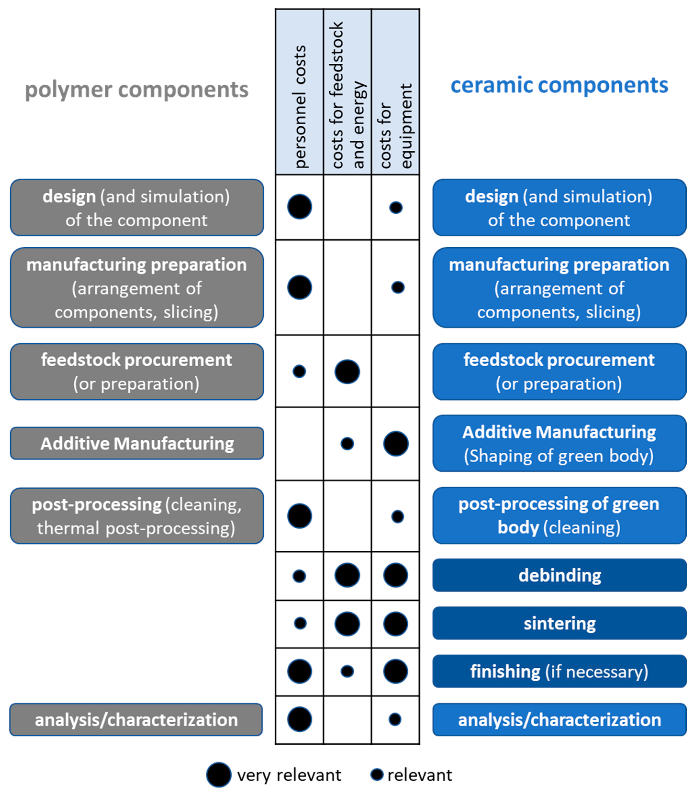
2. Manufacturing Costs for AM Components

2.1. General Considerations

In economic terms, it was and is often claimed that the manufacturing costs of additive manufacturing are independent of the number of pieces produced, as, for example, no costs are required to produce a mold as in injection molding and only material and energy costs are generated for the respective component [13,14]. However, this is not the case. In addition to the variable costs (costs for the feedstock and energy required to manufacture the components), which can be directly allocated to the individual component manufactured, the fixed costs (e.g., depreciation of the equipment, maintenance costs, costs for space requirements) must be allocated to all components manufactured in the time interval under consideration.
Well qualified personnel perform various works, namely purchasing or sales transactions, programming or monitoring equipment, or cleaning or processing components. The costs for the personnel are constantly incurred and are therefore usually included in the fixed costs. Compared to fixed costs, piecework wages and bonuses represent variable costs. However, since this is irrelevant for the general description of the scenario of the cost structure in additive manufacturing, we assign the personnel costs to the fixed costs.
Consequently, the personnel costs must be allocated to the number of manufactured components in the time interval under consideration in the same way as the other fixed costs. Thus, the number of components arranged on one building platform and manufactured in parallel in a print job plays a significant role, since the costs to be allocated decrease as the number of components increases for a constant time interval. This is also considered in many publications, see, e.g., [15,16,17].

2.2. Cost Structure for Indirect and Direct AM Technologies

The multitude of AM technologies can be divided into two different groups—the indirect and the direct AM technologies. The basis for this differentiation is the type of material deposition and consolidation, independent of the material class being processed. This therefore applies to AM of polymers as well as to AM of metals, ceramics, or glasses.
The indirect technologies are characterized by the fact that the material is applied to the entire area of one layer and selectively consolidated [7]. In the case of processes in which the component layers are consolidated for the entire surface at once (e.g., vat photopolymerization (VPP) using digital light processing (DLP)) [18,19,20], the costs for operating the system are completely independent of the number of components placed on the building platform. The necessary manufacturing time and thus the operating costs are defined by the height of the highest component and thus the number of layers to be manufactured. These can be reallocated to more components if the components are arranged more densely.
On the other hand, if we consider the case that a laser is used to solidify the component structures [21], the manufacturing time depends significantly on how much area per layer is to be irradiated and consolidated. Consequently, the manufacturing time increases with the number of components, but the number of green components manufactured per print job can be increased with denser arrangement of the components.
In addition, the upstream (production preparation) and downstream processes (cleaning/embedding) that always occur must also be taken into account. These costs can again be distributed over the number of manufactured components.
In contrast to the indirect AM technologies described above, a direct AM technology deposits the material at the points where it is needed (e.g., Material Extrusion (MEX) [22] and Material Jetting (MJT) [23]) and the manufacturing time depends on the geometry of the components. Direct AM technologies are predestined for the parallel processing of different materials to realize multi-material components, since another material can be deposited immediately next to the deposited one. The manufacturing time and thus the operation costs increase with the number of materials required in the multi-material component and the number of necessary changes between the print heads in the respective layers.
In the case of ceramic components (CerAM, CerAMfacturing [24]), which are followed by thermal processing, the costs for thermal processing are also distributed among the components processed in parallel. Consequently, the manufacturing costs for additively manufactured (ceramic) components also decrease with increasing quantities.

2.3. State-of-the-Art concerning the Component Arrangement

Current software tools (e.g., Magics by Materialise) use the principle of the bounding box for automatic component arrangement. A bounding box is a minimal cuboid-shaped bounding volume, that can contain any given arbitrarily complex 3D shape. The axes of these bounding boxes can be aligned with the pixel grid and the building direction, as is usually the case, or they can be arbitrarily oriented. The maximum expansions of the component parallel to the three spatial directions define the edge length of a cuboid that is stretched around the component. This is then used to arrange the components in relation to each other.
Figure 2 shows an example of the automatically generated arrangement of three different cylinder geometries using the bounding box method. As a boundary condition, the distance between the components or, more precisely, the bounding boxes should be 1 mm in each case. This also applies for the vertically aligned cylinders shown on the right, as the base area of the bounding box corresponds to a square with the dimensions of the cylinder diameter. For the other two component types, where the cylinder geometry is inclined by 15° to the Z-axis, the package density is significantly lower. The reason for this is that the base area of the bounding box in these cases corresponds to a rectangle, whose extension in the y-direction again corresponds to the cylinder diameter but is many times larger in the X-direction. Since the selected distance between the different bounding boxes is set to 1 mm, the real distance between the components is much higher and the packing density is significantly reduced. If the components were also inclined in the Y-direction, the packing density generated by the automatic arrangement using the bounding box method would be reduced even further.
Thus, bounding box nesting has the major drawback that, depending on the component geometry or alignment, the packing density can be limited. A frequently recommended manually nesting, before the software runs automatic nesting algorithms, increases the engineering effort and time.
Currently, an automatic arrangement is used when duplicates of a part are involved and the bounding boxes do not overlap. As soon as different designs are manufactured in one printing job and/or the bounding boxes overlap, manual arrangement is performed to make the best use of the available space. Depending on the number of components, the arrangement can be tedious, and may require 15 min to half an hour. Especially for series production this needs to be improved, because efficient use of the building platform is more critical in this case. For classical prototyping, where typically only individual components are manufactured and the build platform is not fully loaded, there is more flexibility. In addition, less experienced users or operators might face challenges during manual arrangements, which cause a certain entry barrier in terms of the resulting quality of the arrangement and the associated costs. The efficiency and the manufacturing costs are affected by the number of manufactured components per printing job and by the working time of the operator/engineer. Depending on the complexity of the preparation, these engineering costs can mount up to 15 or 20% of the overall manufacturing costs for a given component.
Accordingly, our vision is the development of a software tool that automatically determines the optimal arrangement on one or more building platforms for a given number of components of one or more different geometries and makes it available as machine-readable data. Since its development is very complex, the potential for increasing productivity was first analyzed as part of this work. In what follows, we provide some basic techniques to make this vision a reasonable one.

3. Optimization of Component Arrangement

3.1. Relations to Existing Packing Problems

The goal of producing as many products as possible from a defined quantity of raw materials or semi-finished products and thus maximizing the degree of material utilization has always existed. Typical examples for packing problems are textile semi-finished products (e.g., woven, knitted or warp-knitted fabrics) [25], wooden boards, and container loading [26]. Since the complexity of these problems is related to the product geometry as well as additional constraints, such as the necessary consideration of color gradient or wood grain [27], mathematical optimization algorithms have been used for decades to treat these packing problems.
The optimization of the arrangement of components with uniform or different geometries in a building space of an AM system with the aim of producing as many components as possible in one printing job represents a transfer from a two-dimensional to a three-dimensional arrangement.

3.2. Three Different Arrangement Cases

We distinguish three cases which differ by the required number of components with the same geometry:
  • Case 1. Individual packing: a small number of components with the same or different geometries are needed, arrangement in one building space, manufacturing in one printing job possible.
  • Case 2. Packing for small-scale (small batch) production: many components with the same geometries (hundreds or thousands of each type of geometry) are needed, manufacturing in more than one printing job.
  • Case 3. Packing for bulk (mass) production: with an almost unlimited number of elements of each type, considering the specified percentage for different types of components.
In general, with an increasing number of components and similar printing jobs, the effort for positioning the components can be distributed over a higher number of components and thus the share in the production costs decreases. However, since one of the main advantages of AM is the flexibility to manufacture components with different geometries, cases 1 and 2 occur more frequently and the effort required for component arrangement must be considered.
For the first type of problems, heuristics methods can be applied, e.g., optimization by groups of variables [28], bottom-left technique [29]. The second and third type of problems can be solved using regular (lattice) and sectional-regular packing [30,31,32].
Within this paper we address case 2 and case 3 to demonstrate the potential of mathematical algorithms concerning the optimization of the arrangement of the components for AM processes.
It is extremely difficult to solve somewhat large instances of packing problems exactly [33]. Therefore, we propose a heuristic approach that is based on mathematical modelling of placement conditions.
Different geometric tools and models for solving packing problems are reviewed in [34]. The most powerful tool of analytical description of interactions of 2D and 3D objects under free translations and rotations in packing problems is the phi-function technique [28,35,36]. The operation of phi-functions is explained in more detail in Appendix A.
The phi-function technique has been successfully used for modeling different packing problems that arise in a wide spectrum of applications, e.g., space engineering, biomedicine, material sciences, medicine, nanotechnologies (to mention just a few). Some original developments are related to additive manufacturing as follows: for cleaning parts produced by 3D printing from non-sintered particles using the terminal deburring method [37]; for topological optimization of 3D parts by generating void structure [38]; for optimization of the occupied volume of the printing chamber; for computer simulation of material structures used to obtain high-quality and durable parts by 3D printing [39].

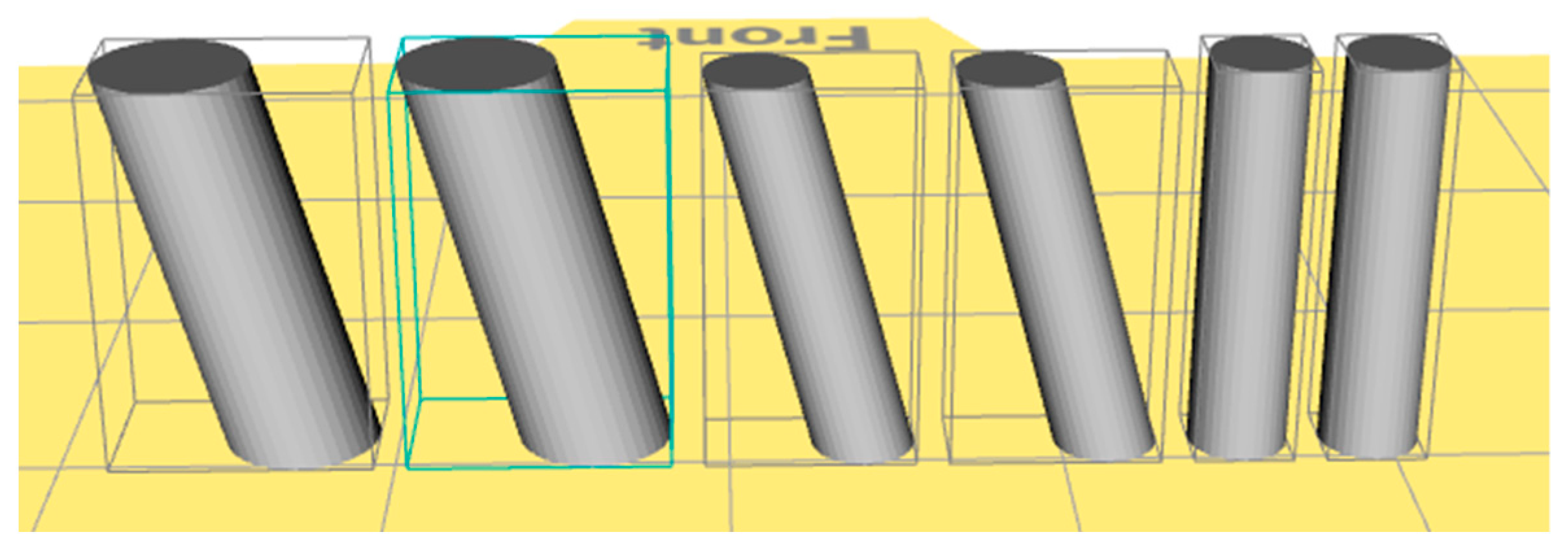
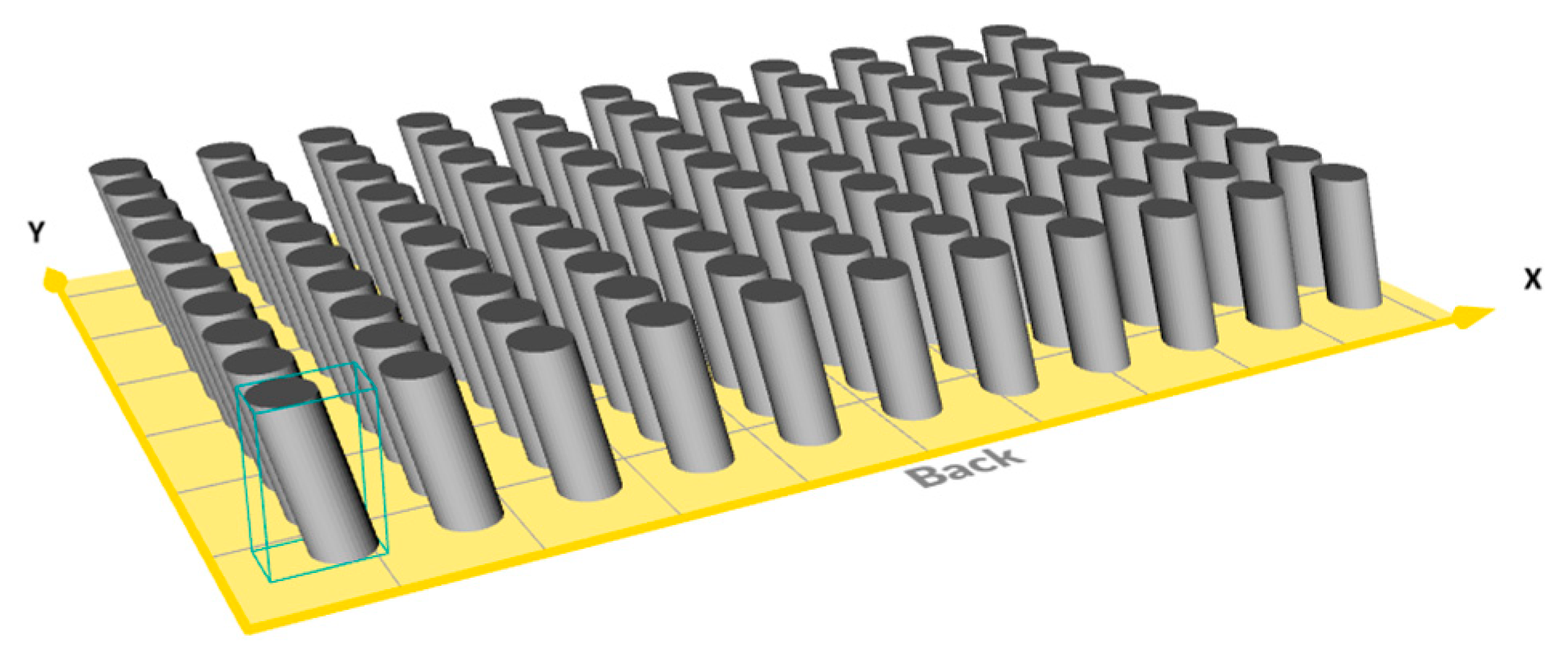
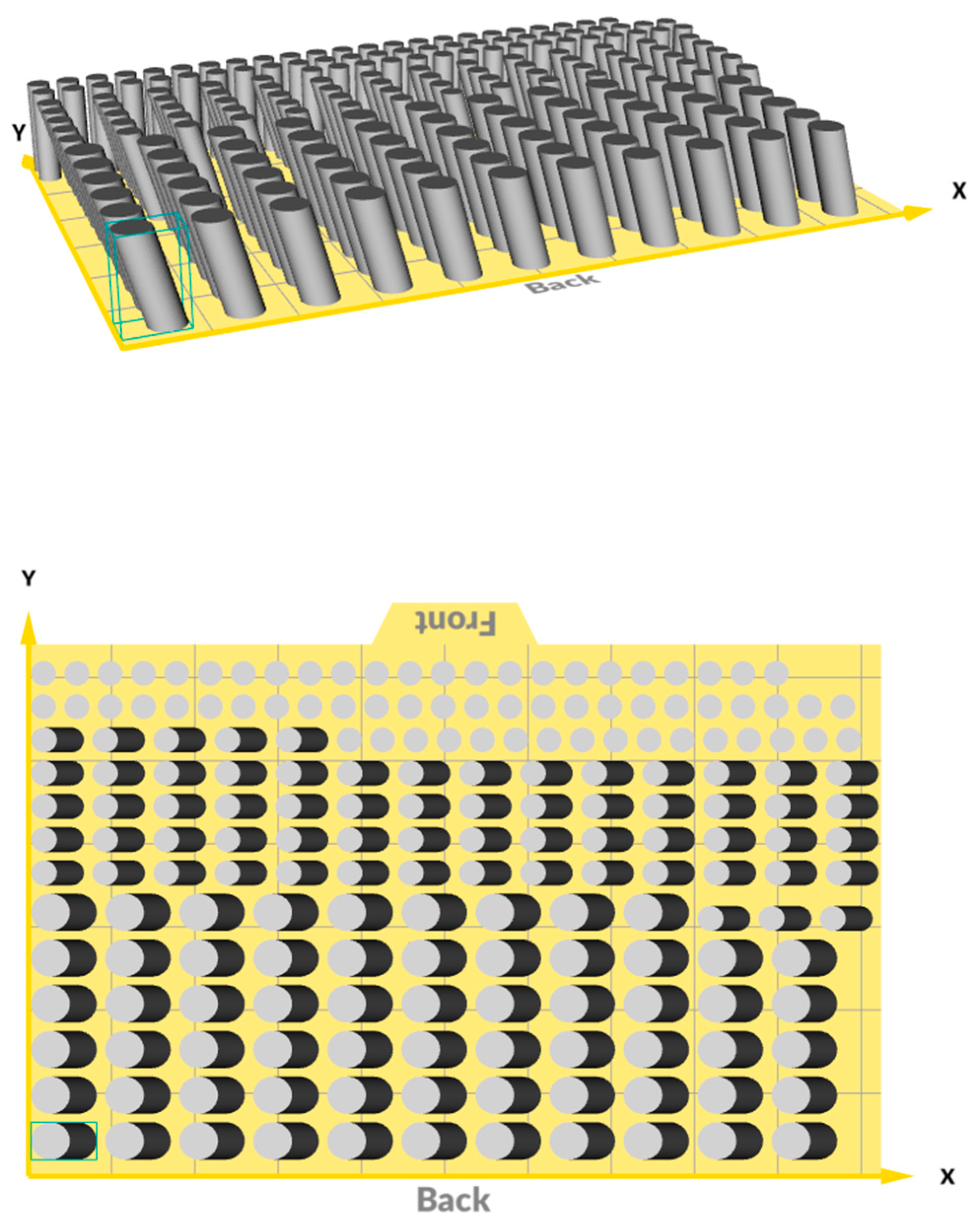
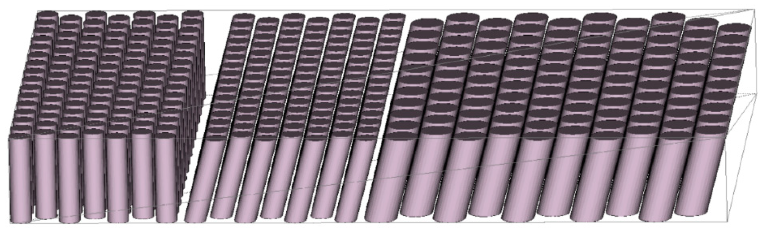
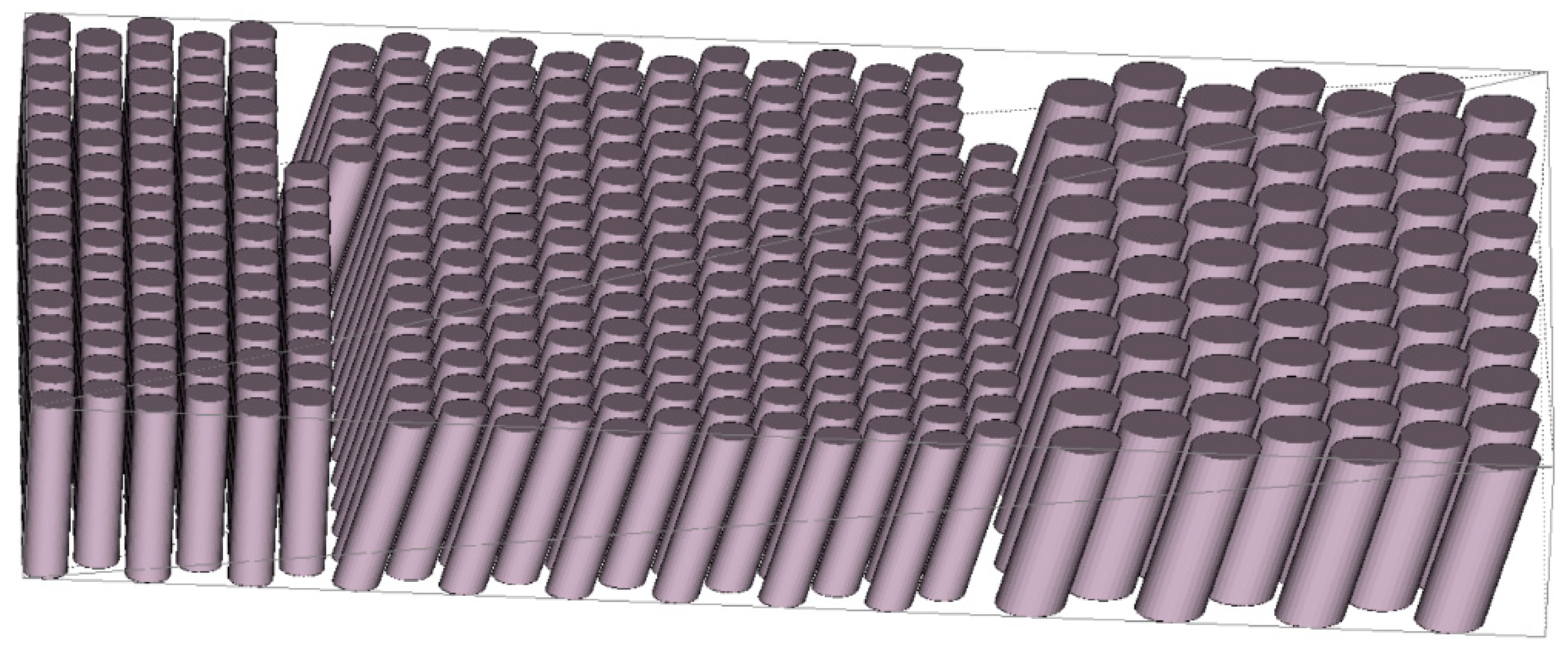
3.3. Boundary Conditions and an Exemplary Task for Demonstration

The building space is a cuboidal container of given sizes (dimensions). All components to be arranged are convex (in general oblique 3D) objects; the types of objects describe components with different geometries. For the arrangement of components, they are allowed to move on the bottom of the cuboidal container according to the following placement conditions:
  • non-overlapping of components taking into account minimal allowable distances between each pair of components;
  • containment of components in the cuboidal container.
The objective is to minimize the number of printing jobs needed for a given number of components of several types subject to the placement conditions.
We have chosen a simple example for illustration. Three types of cylinders with different geometries have to be arranged on the building platforms in such a way that the number of print jobs required to manufacture approx. 1000 cylinders of each type is reduced. Table 1 summarizes the geometrical parameters for the selected cylinder geometries (CG).
The following Figure 3, Figure 4 and Figure 5 show the arrangement of the components with the current automatic software tool of a Lithoz device [18,19], which uses the principle of the bounding box, with the boundary conditions in that the distance between the individual components is always 1 mm and that the maximum number of components of one type is arranged on the building platform. The size of the building platform is 102 mm × 64 mm which is similar to the real building platform size of a CeraFab 8500 of Lithoz.
Within the current automatic software tool, it is not possible to load the component geometry and then have the maximum packing created according to the boundary condition. The user must define a number of components, have the arrangement generated and then check it to see how many components will fit on the platform and whether the number of components can be increased or needs to be reduced.
Figure 6 shows an alternative arrangement of the components. The boundary condition is that the same number of components of all three types must be arranged together on one building platform. To generate this arrangement, we started with a number of 70 components per type and then iteratively reduced the number of components until they all fitted on one building platform.
Table 2 summarizes the maximum number of components of the different types per building platform for the different scenarios. In addition, the number of building platforms needed to manufacture approx. 1000 components per type is calculated. If only one geometry per building platform is manufactured, approx. 17 building platforms are necessary; with the strategy of arranging the three different types with the same number each on one building platform, 16 are necessary.

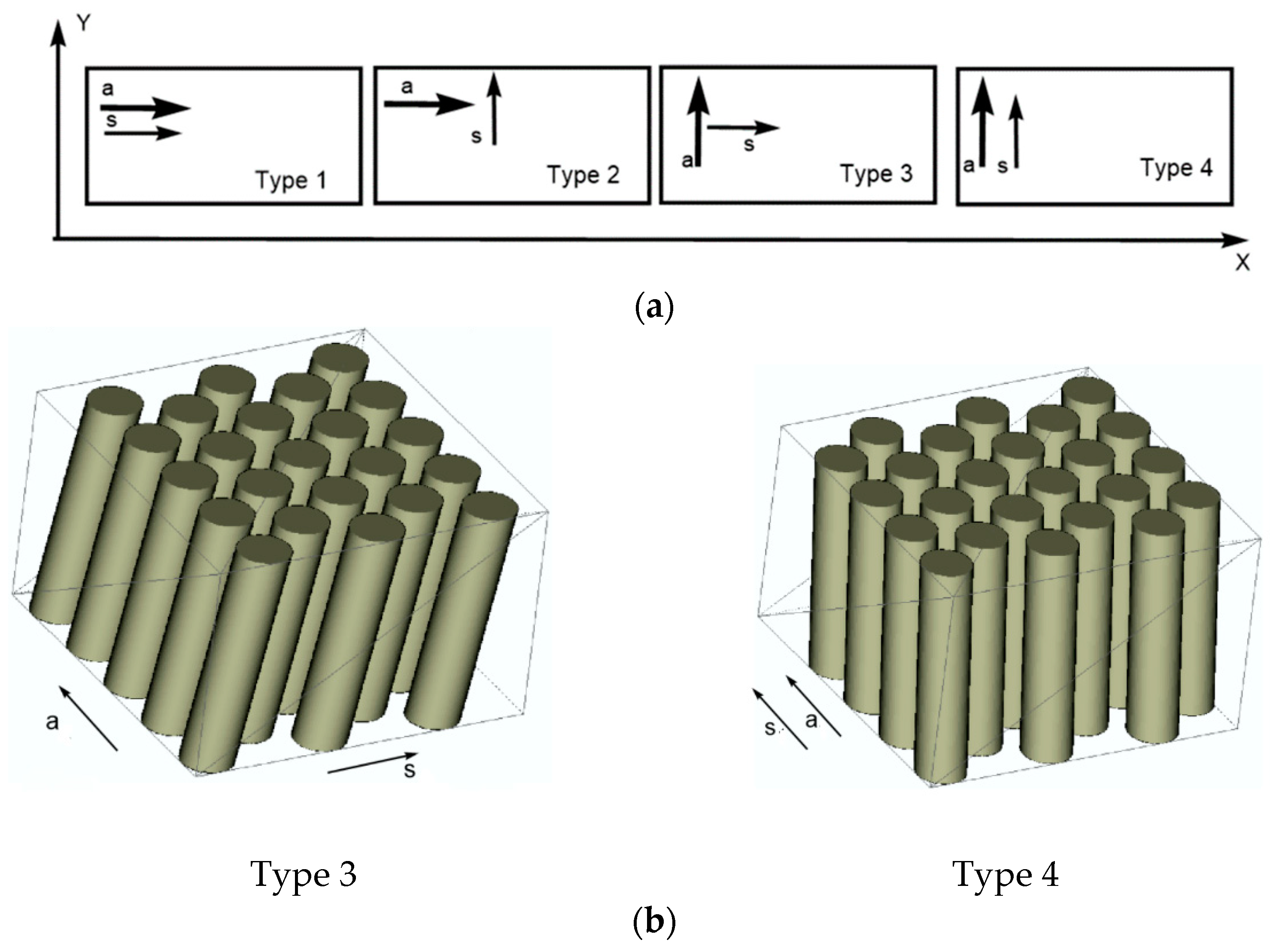
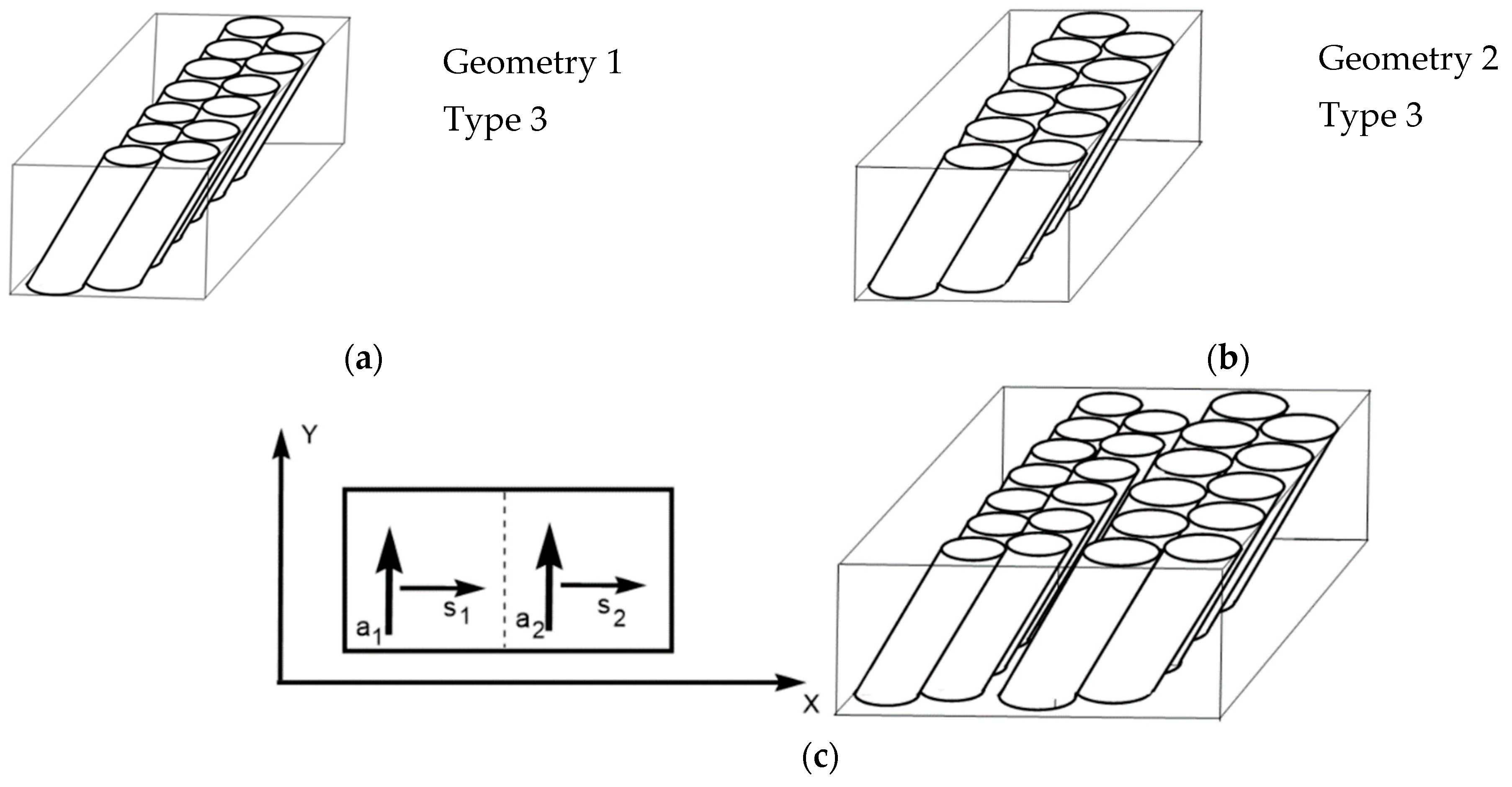
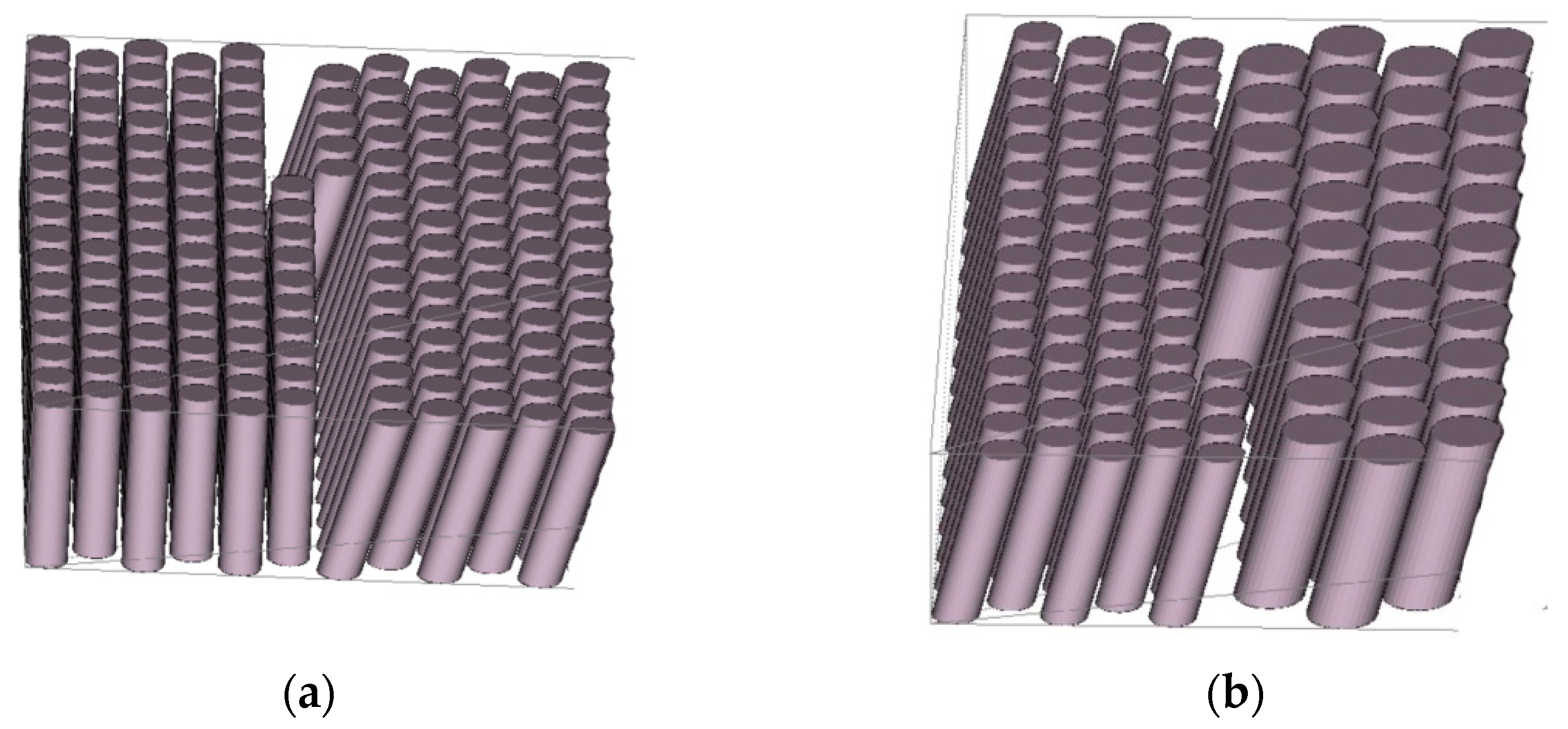
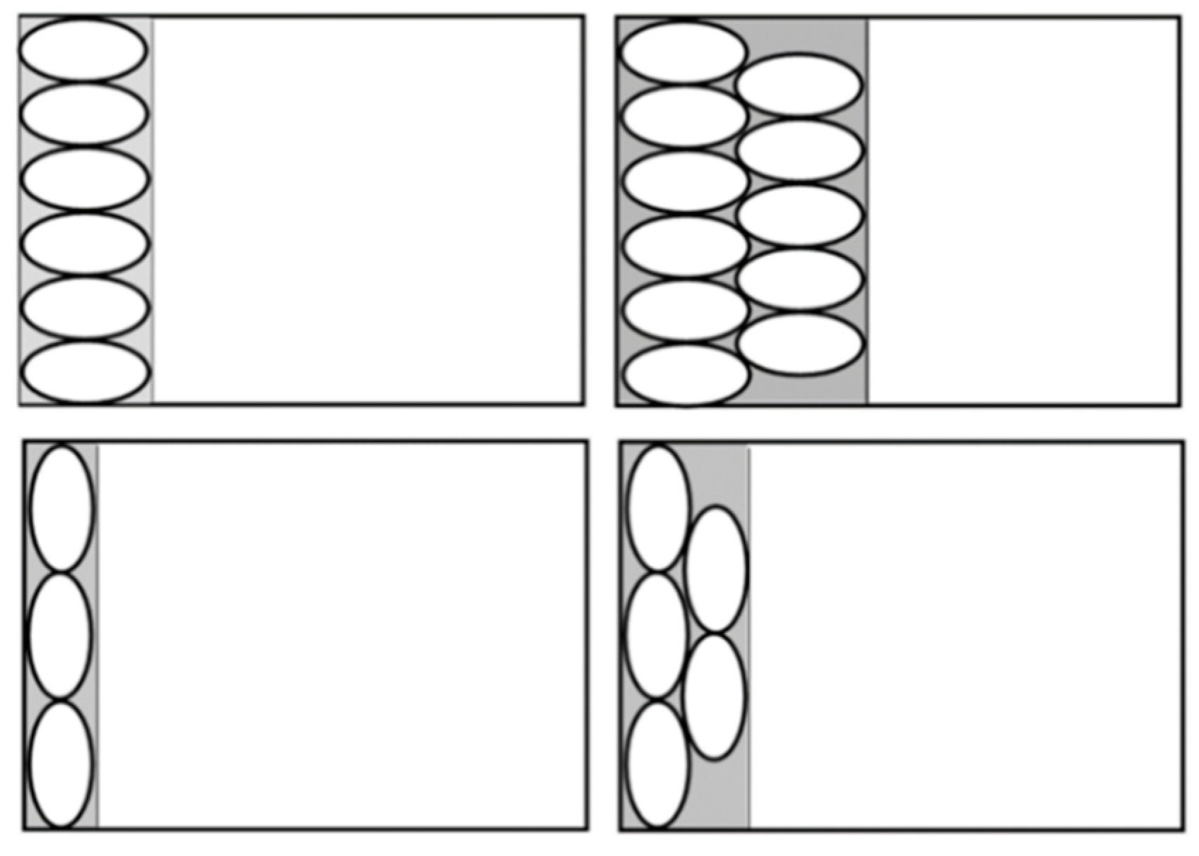
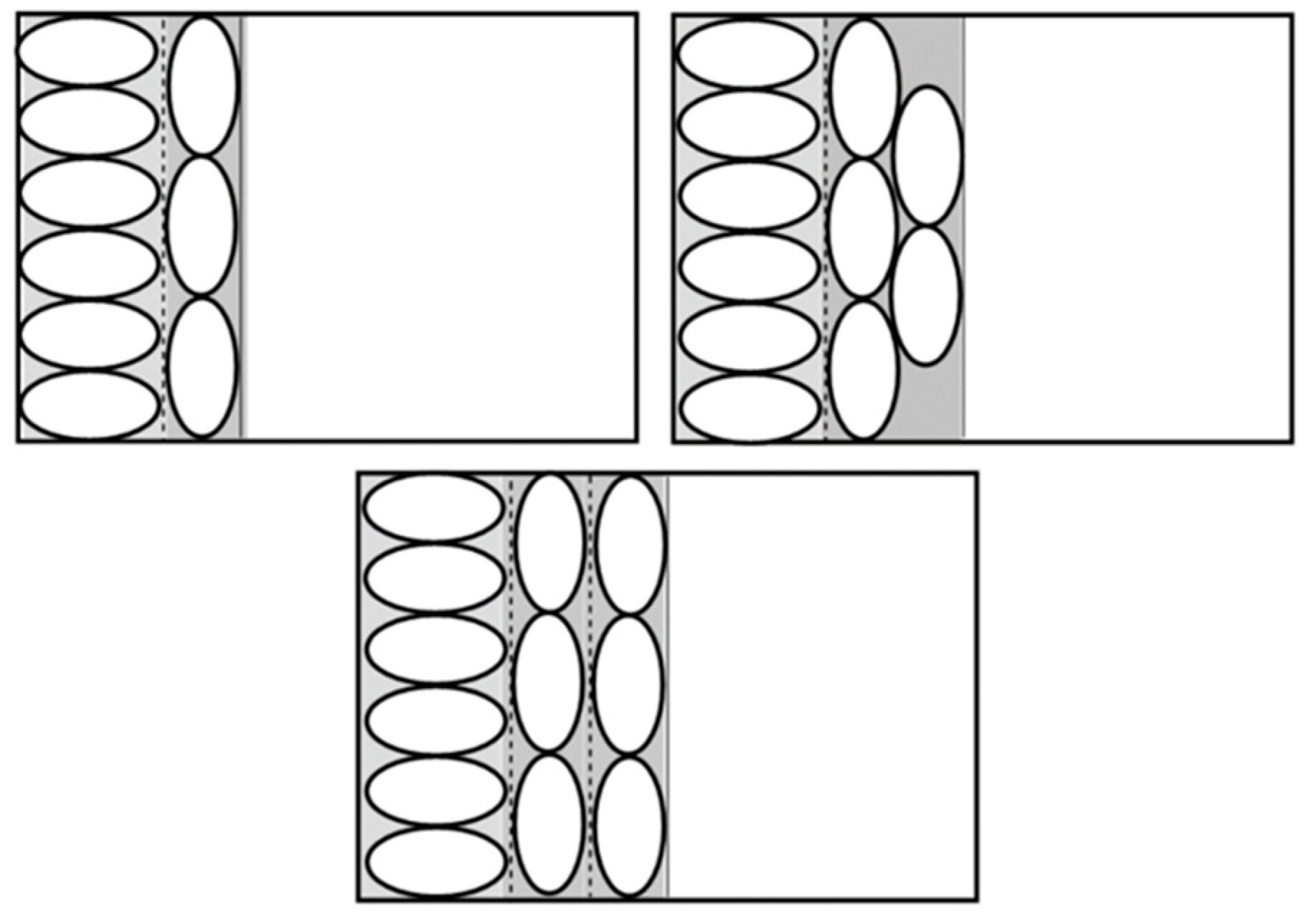
4. New Approach: Regular-Sectional Arrangement

An efficient way to arrange components with the same geometry is regular packing (lattice packing). The bases of identically oriented non-overlapping 3D components of the same type are placed on the plane at the nodes of a lattice, provided that the first vector of the basis of the lattice is parallel to one of the sides of the base of the cuboid. An example of a lattice is provided in Figure 7.
For describing non-overlapping of components with minimal allowable distances, adjusted quasi-phi-functions for appropriate geometries are used while phi-functions for containment of components in the cuboidal container are applied (see Appendix A and Figure 8).
To reduce the number of components for the calculation and modeling, sectional-regular packing can be employed. A cuboid is divided into sections by vertical planes parallel to one of the sides of the cuboid base. Each of the cuboidal sections is packed regularly.

4.1. Main Scenario and Techniques

First, the lattice parameters are calculated with a predefined step. For each type of geometry, taking into account the given number of desired components, a minimum-volume section is constructed that contains regular packing of these components. The parameters of the best section are chosen. In a particular case, the best section may coincide with the original cuboid.
Second, the best packing of a set of sections is found. The packing provides the placement of all components (or a certain number of components) while considering a given ratio of the numbers of different geometries.
Considering that inclined components are used, let us define possible types of regular packing of sections. For each section we consider the following:
(1)
two alternative directions (a horizontal or a vertical) of the first vector of the lattice base along X-axis or Y-axis (shown in Figure 9a by arrow a);
(2)
two alternative directions (a horizontal or a vertical) of the object inclination along X-axis or Y-axis (shown in Figure 9a by arrow s).
Therefore, for each geometry, we have four different types of sections in terms of directions (see diagram in Figure 9a). Figure 9b shows examples of two types of sections for the same geometry.
Now we define possible variants for combining two sections with possibly different geometries.
Two sections with different geometries (Geometry 1 and Geometry 2) can be combined in 24 = 16 different ways (variants of combinations of sections). We assume that the directions of the first vectors of the two lattice bases (a1 for Geometry 1 and a2 for Geometry 2) must be the same. Therefore, for each pair of sections, we have 8 variants for their combination (Figure 10a). Here, index 1 or 2 is related to the appropriate geometry. Another presentation of the possible combinations of a pair of sections is given in Figure 10b.
The distance between sections can be reduced if they are considered in order of non-decreasing inclination angle of the components. In this case, the upper parts of the components of the last row of the section will hang over the components of the first row of the next section (Figure 11).
In addition, a “swap” technique for arrangement of sections with the same type of components is applied, if they are simultaneously ordered by increasing the component sizes and inclination angle.
The key idea of the technique is replacing a given number of components of a larger size and/or with a larger inclination angle by the corresponding number of components of a smaller size and/or with a smaller angle. In this case, an overlapping of sections is allowed (see Figure 12).

4.2. Solution Algorithm

The solution strategy for large-scale problems involves three main stages. At stage 1, the rotation angle, length, and orientation (parallel to one of the sides of the container) of each type of object are defined. The vector of the lattice basis is constructed, and all possible sections of each possible size are generated for each basis (Figure 13).
For each section, the type of objects, the number of objects, the rotation angle of the lattice basis, as well as the section dimensions are stored. If two sections have the same object type as well as the same number of objects, then the section with a smaller size is stored.
During stage 2, an attempt is made for each type of object to construct combined sections, using dynamic programming for solving the one-dimensional knapsack problem (Figure 14).
Information about a combined section involves the type of objects, the number of objects, the size of the section, and a “link” to two related “section ancestors”. As in the previous case, only sections that are minimal in size are stored (comparison with simple sections is also realized).
At stage 3, the minimal number of objects is estimated (subject to the given ratio constraints) for which there exists regular packing in the container. Starting from this number, the sequential generation of increasing numbers of objects for each ratio is realized and then the corresponding problems of small-scale packing (the batch production) are solved. The best variants are stored. The procedure continues until the desirable efficiency is reached.
A solution strategy for small-scale packing is the following. First, a set of optimized sections are constructed. Sections in which the number of components exceeds the number of unplaced components of the corresponding type are excluded from further consideration. Second, a greedy algorithm for generating packings of sections on the building platform is used. From the available set of sections, the best packing is constructed using dynamic programming. The “greed” of the algorithm can be monitored using weight coefficients. The resulting packing is saved, and the number of unplaced components is changed. The procedure is repeated until all unplaced components are arranged.

5. Results and Discussion

Figure 15 shows one arrangement of the three different types of components, if the same number of components for each type have to be placed on the building platform.
In this solution, 109 components of each type could be arranged. This solution makes it possible to manufacture 981 and 1100 components of each type with nine and ten printing jobs respectively (Table 3). Compared to the solution obtained by the current automatic software tool, this corresponds to a 70% increase in the number of components on a building platform or a 44% reduction in the number of building platforms needed to manufacture 980 components of each type.
However, it is possible to change the arrangement so that even more components can be manufactured in the same time. In Table 4 and Table 5, the number of components that are manufactured during the respective printing jobs are summarized. Figure 16, Figure 17, Figure 18, Figure 19, Figure 20 and Figure 21 show the corresponding arrangement of the components.
It is therefore possible to increase the number of manufactured components by approx. 1%, solely by rearranging the components without changing their distances in any way.
Now this is not another significant increase over the component arrangements described above. However, this does illustrate very well that the optimal solution is very difficult to determine by simple reasoning and a human operator would spend much more time on optimization than a mathematical algorism requires.

6. Conclusions

In this work, we showed that mathematical methods turn out to be an important tool for optimizing the arrangement of the components on a building platform. Thus, the number of components manufactured in one or many printing jobs can be considerably increased. This results directly in a significant decrease in the manufacturing costs for the components. For the selected example of geometries and boundary conditions, an increase in building platform utilization of 70% and a decrease in the number of printing jobs by 44% could be achieved.
With increasing geometric complexity (e.g., Figure 22) as well as the number of different component geometries to be manufactured and the number of printing jobs required for manufacturing, the effort required to optimize the arrangement of the individual components increases. An automated method can contribute to significant savings in time and costs. The phi-function technique can be used for analytical description of non-overlapping and distance constraints for differently shaped objects (see, e.g., [40]).
Such optimization is also possible for components whose outer surfaces cannot be approximated by a single simple geometric structure. For this purpose, special phi functions are used, which treat irregular objects as a union of basic shapes (see Appendix A).
To optimize the manufacturing preparation for AM components, the following three-step method is proposed:
  • Preparation-analysis and abstraction of the component geometry:
    • an assessment of the manufacturability of the component as a function of the orientation on the build platform (manufacturability/probability of defect/…) is made in order to limit the number of possibilities for positioning the components during optimization of the feasible variants;
    • an abstraction of the outer geometry of the components by simple three-dimensional geometries (sphere, cylinder, cuboid, tetrahedron, …) is carried out in order to reduce the computational effort.
  • Optimization of the component arrangement:
    • the arrangement of the (abstracted) components is optimized, whereby the (abstracted) components can be rotated around all three spatial axes;
    • the specification of boundary conditions for the optimization takes place (e.g., (minimum) distance of the components to each other, desired number (interval), desired construction height/production time, …);
    • a weighting of the boundary conditions can be carried out;
    • optimization can be carried out according to several target variables/(weighted) boundary conditions.
  • Generation of the CAM data:
    • reconversion of the abstracted geometries into the original geometries;
    • machine data are generated.

Author Contributions

Conceptualization, U.S. and T.R.; methodology, U.S., T.R., F.E. and M.S.; mathematically investigation T.R. and O.P.; writing—original draft preparation, U.S. and T.R; writing—review and editing, E.S.-F., M.S. and A.F.; visualization, E.S.-F. and T.R. All authors have read and agreed to the published version of the manuscript.

Funding

The second and the last author (Tetyana Romanova and Andreas Fischer) were supported by the Volkswagen Foundation under grant numbers 97775 and 9C086.

Institutional Review Board Statement

Not applicable.

Informed Consent Statement

Not applicable.

Data Availability Statement

Not applicable.

Acknowledgments

The authors thank Susanne Pötzsch for creating and providing the hand drawings that were used in Figure 8. In addition, we would like to thank Lutz Gollmer for his assistance in considering the manufacturing costs as well as the preparation of Figure 1.

Conflicts of Interest

The authors declare no conflict of interest.

Appendix A

Appendix A.1. Modeling of Basis Geometric Constraints in Packing Problems
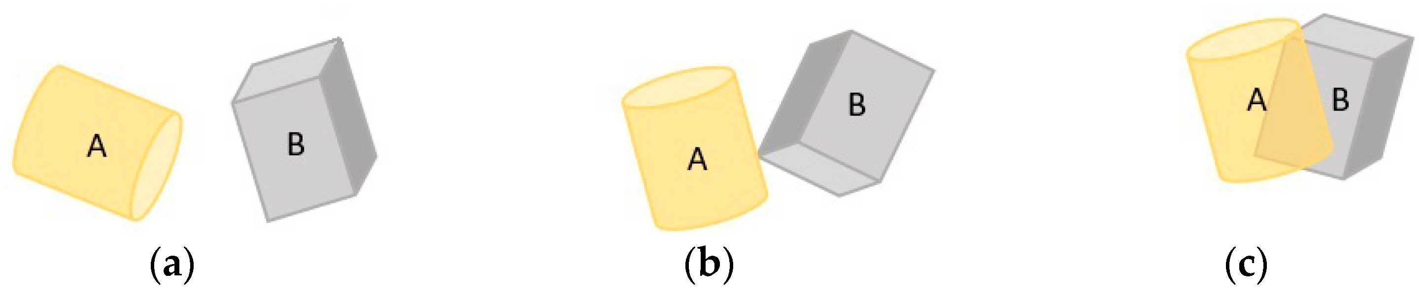
Let us consider two objects A R σ and B R σ of the given shapes and sizes, σ = 2 , 3 . Denote a given container by Ω σ .
The basic placement conditions in a packing problem are:
  • non-overlapping condition: A and B do not intersect, but can touch each other, i.e., int A int B = ;
  • containment condition: A is arranged fully inside the container Ω , i.e., A Ω ;
  • distance condition: the distance between objects A and B is grater than or equal to ρ , i.e.,
    d i s t ( A , B ) ρ
    where ρ > 0 , d i s t ( A , B ) = min a A , b B d ( a , b ) , d ( a , b ) stands for the Euclidean distance between two points a , b R σ .
To describe the placement conditions analytically, the phi-function technique [28,35] is used.
This technique guarantees that the distance between two objects does not fall below a predefined minimal allowable value. It also guarantees that an object belongs to the building space.

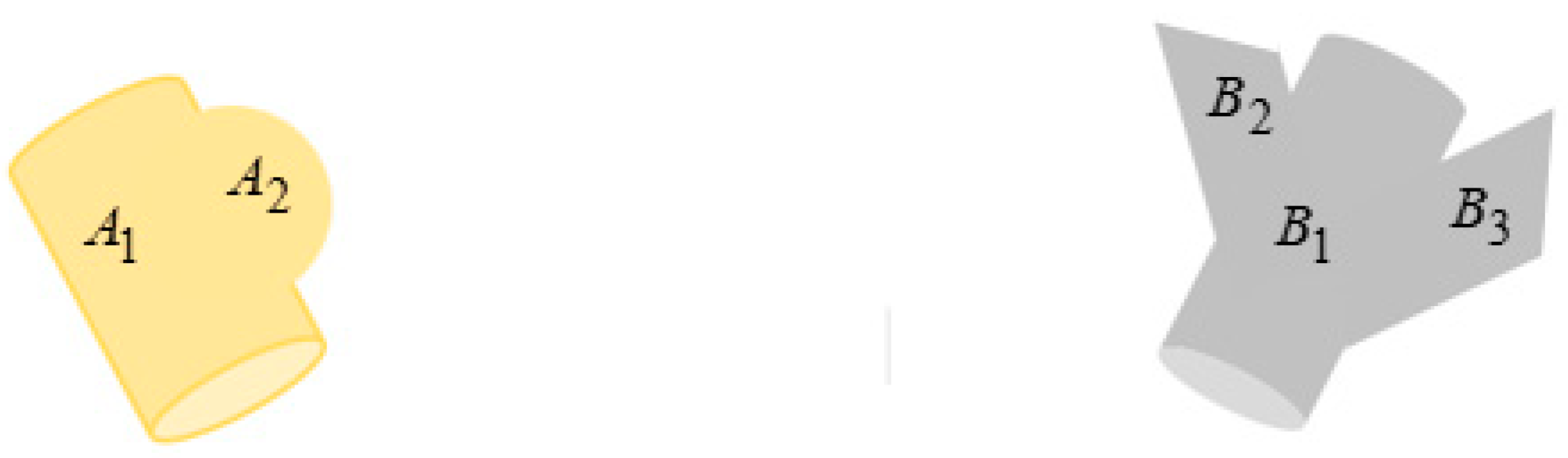
Appendix A.2. Basic Definitions of the phi-Function Technique

Definition 1
[28]. A continuous and everywhere defined function  Φ A B ( u A , u B ) is called a phi-function for objects  A ( u A )  and  B ( u B )  if Φ A B ( u A , u B )  is positive for cases when objects  A  and  B do not overlap (see Figure A1, case a), Φ A B ( u A , u B ) is 0 for cases when objects A and B touch (see Figure A1, case b), Φ A B ( u A , u B ) is negative for cases when objects A and B overlap (see Figure A1, case c). Here u A , u B are the appropriate variable motion vectors of A and B .
Figure A1. A phi-function differentiates three cases of mutual arrangements of a pair of objects: (a) no common points; (b) common boundary points only; (c) common interior points.
Ceramics 06 00038 g0a1
Thus, non-overlapping means Φ A B ( u A , u B ) 0 .

Appendix A.3. Adjusted phi-Function

Let a minimal allowable distance ρ > 0 between A and B be given.
Definition 2
[28]. A continuous and everywhere defined function  Φ A B ( u A , u B ) is called an adjusted phi-function for objects A ( u A ) and B ( u B ) , if Φ ( u A , u B ) is positive for cases when the distance between objects A and B is grater than ρ (see Figure A2, case a), Φ A B ( u A , u B ) is 0 for cases when the distance between objects A and B is equal to ρ (see Figure A2, case b), Φ A B ( u A , u B ) is negative for cases when the distance between objects A and B is less than ρ (see Figure A2, case c).
Therefore, distance condition means Φ A B ( u A , u B ) 0 .
Figure A2. An adjusted phi-function differentiates three cases of mutual arrangements of a pair of objects: (a) distance between objects is greater than ρ ; (b) distance between objects is equal to ρ ; (c) distance between objects is less than ρ .
Ceramics 06 00038 g0a2
Ready-to-use phi-functions are provided for 2D objects bounded by arcs and line segments in [41], for ellipses in [42], for 3D objects including spheres, cuboids, cylinders, cones, and polyhedra in [43], for ellipsoids in [44], for some oblique 3D shapes in [40].

Appendix A.4. Phi-Function for Irregular Objects Composed by a Union of Basic Shapes

Let A ( u A ) = i = 1 n A i ( u A ) and B ( u B ) = j = 1 m B j ( u B ) and Φ i j ( u A , u B ) be a known phi-function for basic objects A i ( u A ) and B j ( u B ) . Then a phi-function for irregular objects A ( u A ) and B ( u B ) can be defined in the form Φ A B ( u A , u B ) = min i = 1 , , n , j = 1 , , m Φ i j ( u A , u B ) . An adjusted phi-function for the composed objects is defined in the same way.
For example, a phi-function for objects A = A 1 A 2 and B = B 1 B 2 B 3 provided in Figure A3 has the form Φ A B = min { Φ 11 , Φ 12 , Φ 13 , Φ 21 , Φ 22 , Φ 23 } , where A 1 is a right cylinder, A 2 is a sphere, B 1 is a right cylinder, B 2 , B 3 are oblique cylinders, Φ 11 , Φ 12 , Φ 13 , Φ 21 , Φ 22 , Φ 23 are phi-functions for the appropriate pair of objects: A 1 , B 1 ;   A 1 , B 2 ;   A 1 , B 3 ;   A 2 , B 1 ;   A 2 , B 2 ;   A 2 , B 3 .
Figure A3. Examples of two composed objects.
Ceramics 06 00038 g0a3

References

  1. Gries, S.; Meyer, G.; Wonisch, A.; Jakobi, R.; Mittelstedt, C. Towards Enhancing the Potential of Injection Molding Tools through Optimized Close-Contour Cooling and Additive Manufacturing. Materials 2021, 14, 3434. [Google Scholar] [CrossRef] [PubMed]
  2. Hybrid Metal 3D Printer Redefines Mold Component Production. Available online: https://www.moldmakingtechnology.com/products/hybrid-metal-3d-printer-redefines-mold-component-production (accessed on 29 January 2023).
  3. Achinas, S.; Heins, J.I.; Krooneman, J.; Euverink, G.J.W. Miniaturization and 3D Printing of Bioreactors: A Technological Mini Review. Micromachines 2020, 11, 853. [Google Scholar] [CrossRef]
  4. Fujimoto, K.T.; Hone, L.A.; Manning, K.D.; Seifert, R.D.; Davis, K.L.; Milloway, J.N.; Skifton, R.S.; Wu, Y.; Wilding, M.; Estrada, D. Additive Manufacturing of Miniaturized Peak Temperature Monitors for In-Pile Applications. Sensors 2021, 21, 7688. [Google Scholar] [CrossRef]
  5. Realizing the Benefits of Miniaturization of Electronic Components with 3D Printing. Available online: https://www.nano-di.com/resources/blog/2020-realizing-the-benefits-of-miniaturization-of-electronic-components-with-3d-printing (accessed on 29 January 2023).
  6. Chen, Z.; Li, Z.; Li, J.; Liu, C.; Lao, C.; Fu, Y.; Liu, C.; Li, Y.; Wang, P.; He, Y. 3D printing of ceramics: A review. J. Eur. Ceram. Soc. 2019, 39, 661–687. [Google Scholar] [CrossRef]
  7. Zocca, A.; Colombo, P.; Gomes, C.M.; Günster, J. Additive manufacturing of ceramics: Issues, potentialities, and opportunities. J. Am. Ceram. Soc. 2015, 98, 1983–2001. [Google Scholar] [CrossRef]
  8. Travitzky, N.; Bonet, A.; Dermeik, B.; Fey, T.; Filbert-Demut, I.; Schlier, L.; Schlordt, T.; Greil, P. Additive Manufacturing of ceramic-based material. Adv. Eng. Mater. 2014, 16, 729–754. [Google Scholar] [CrossRef]
  9. Tan, C.K.L.; Goh, Z.H.; De Chua, K.W.; Kamath, S.; Chung, C.K.R.; Teo, W.B.Y.; Martinez, J.C.; Dritsas, S.; Simpson, R.E. An improved hearing aid fitting journey; the role of 3D scanning, additive manufacturing, and sustainable practices. Mater. Today Proc. 2022, 70, 504–511. [Google Scholar] [CrossRef]
  10. How Personalization Has Changed the Hearing Aid Industry for the Better. Available online: https://www.materialise.com/en/inspiration/cases/phonak-3d-printed-hearing-aid (accessed on 29 January 2023).
  11. Top Seven Industries for Additive Manufacturing Applications. Available online: https://luxcreo.com/top-seven-industries-for-additive-manufacturing-applications/ (accessed on 29 January 2023).
  12. Additive Manufacturing: Applications by Sector. Available online: https://www.3dnatives.com/en/applications-by-sector/# (accessed on 29 January 2023).
  13. Hopkinson, N.; Dicknes, P. Analysis of rapid manufacturing—Using layer manufacturing processes for production. Proc. Inst. Mech. Eng. Part C J. Mech. Eng. Sci. 2003, 217, 31–39. [Google Scholar] [CrossRef] [Green Version]
  14. 3D Printing Manufacturing Costs. Available online: https://multec.de/en/3d-printing-technology/production-costs-of-3d-printed-parts (accessed on 8 December 2022).
  15. Ruffo, M.; Tuck, C.; Hague, R.J.M. Cost estimation for rapid manufacturing—Laser sintering production for low to medium volumes. Proc. Inst. Mech. Eng. Part B J. Eng. Manuf. 2006, 220, 1417–1427. [Google Scholar] [CrossRef] [Green Version]
  16. Thomas, D.; Gilbert, S. Costs and Cost Effectiveness of Additive Manufacturing; Special Publication (NIST SP), National Institute of Standards and Technology: Gaithersburg, MD, USA, 2014. [CrossRef]
  17. Thomas, D. Costs, benefits, and adoption of additive manufacturing: A supply chain perspective. Int. J. Adv. Manuf. Technol. 2016, 85, 1857–1876. [Google Scholar] [CrossRef] [Green Version]
  18. Homa, J. Rapid prototyping of high-performance ceramics opens new opportunities for the CIM industry. Powder Inject. Mould. Int. 2012, 6, 65–68. [Google Scholar]
  19. Schwentenwein, M.; Homa, J. Additive manufacturing of dense alumina ceramics. Int. J. Appl. Cer. Technol. 2015, 12, 1–7. [Google Scholar] [CrossRef]
  20. Halloran, J.W. Ceramic stereolithography: Additive manufacturing for ceramics by photopolymerization. Annu. Rev. Mater. Res. 2016, 46, 19–40. [Google Scholar] [CrossRef]
  21. Griffith, M.L.; Halloran, J.W. Freeform fabrication of ceramics via stereolithography. J. Am. Ceram. Soc. 1996, 79, 2601–2608. [Google Scholar] [CrossRef] [Green Version]
  22. Abel, J.; Scheithauer, U.; Janics, T.; Hampel, S.; Cano, S.; Müller-Köhn, A.; Günther, A.; Kukla, C.; Moritz, T. Fused Filament Fabrication (FFF) of Metal-Ceramic Components. J. Vis. Exp. 2018, 143, e57693. [Google Scholar]
  23. Weingarten, S.; Scheithauer, U.; Johne, R.; Abel, J.; Schwarzer, E.; Moritz, T.; Michaelis, A. Multi-material Ceramic-Based Components—Additive Manufacturing of Black-and-white Zirconia Components by Thermoplastic 3D-Printing (CerAM-T3DP). J. Vis. Exp. 2019, 143, e57538. [Google Scholar] [CrossRef] [Green Version]
  24. Michaelis, A.; Scheithauer, U.; Moritz, T.; Weingarten, S.; Abel, J.; Schwarzer, E.; Kunz, W. Advanced Manufacturing for Advanced Ceramics. Procedia CIRP 2020, 95, 18–22. [Google Scholar] [CrossRef]
  25. Terno, J.; Lindemann, R.; Scheithauer, G. Zuschnittprobleme und Ihre Praktische Lösung. Mathematische Modelle von Layout-Problemen, 1st ed.; Harri Deutsch: Frankfurt/Main, Germany, 1987. [Google Scholar]
  26. Scheithauer, G. Algorithms for the Container Loading Problem. In Operations Research Proceedings; Gaul, W., Bachem, A., Habenicht, W., Runge, W., Stahl, W.W., Eds.; Springer: Berlin/Heidelberg, Germany, 1991; pp. 445–452. [Google Scholar] [CrossRef]
  27. Fischer, A.; Scheithauer, G. Cutting and Packing Problems with Placement Constraints. In Optimized Packings with Applications; Fasano, G., Pinter, J.D., Eds.; Springer: Cham, Switzerland, 2015; pp. 119–156. [Google Scholar]
  28. Chernov, N.; Stoyan, Y.; Romanova, T. Mathematical model and efficient algorithms for object packing problem. Comput. Geom. Theory Appl. 2010, 43, 535–553. [Google Scholar] [CrossRef] [Green Version]
  29. Burke, E.K.; Hellier, R.S.R.; Kendall, G.; Whitwell, G. A New Bottom-Left-Fill Heuristic Algorithm for the Two-Dimensional Irregular Packing Problem. Oper. Res. 2006, 54, 587–601. [Google Scholar] [CrossRef] [Green Version]
  30. Stannarius, R.; Schulze, J. On regular and random two-dimensional packing of crosses. Granul. Matter 2022, 24, 25. [Google Scholar] [CrossRef]
  31. Kallus, Y.; Kusner, W. The Local Optimality of the Double Lattice Packing. Discret. Comput. Geom. 2016, 56, 449–471. [Google Scholar] [CrossRef] [Green Version]
  32. Milenkovic, V.J. Densest translational lattice packing of non-convex polygons. Comput. Geom. Theory Appl. 2002, 22, 205–222. [Google Scholar] [CrossRef] [Green Version]
  33. Chazelle, B.; Edelsbrunner, H.; Guibas, L.J. The complexity of cutting complexes. Discret. Comput. Geom. 1989, 4, 139–181. [Google Scholar] [CrossRef] [Green Version]
  34. Leao, A.S.; Toledo, F.M.B.; Oliveira, J.F.; Carravilla, M.A.; Alvarez-Valdés, R. Irregular packing problems: A review of mathematical models. Eur. J. Oper. Res. 2020, 282, 803–822. [Google Scholar] [CrossRef]
  35. Stoyan, Y.; Pankratov, A.; Romanova, T. Quasi-phi-functions and optimal packing of ellipses. J. Glob. Optim. 2016, 65, 283–307. [Google Scholar] [CrossRef]
  36. Kallrath, J. Business Optimisation Using Mathematical Programming. In Cutting & Packing beyond and within Mathematical Programming, 2nd ed.; Springer: Cham, Switzerland, 2021; Chapter 15; pp. 495–526. [Google Scholar]
  37. Romanova, T.; Stoyan, Y.; Pankratov, A.; Litvinchev, I.; Plankovskyy, S.; Tsegelnyk, Y.; Shypul, O. Sparsest balanced packing of irregular 3D objects in a cylindrical container. Eur. J. Oper. Res. 2021, 291, 84–100. [Google Scholar] [CrossRef]
  38. Romanova, T.; Stoyan, Y.; Pankratov, A.; Litvinchev, I.; Avramov, K.; Chernobryvko, M.; Yanchevskyi, I.; Mozgova, I.; Bennell, J. Optimal layout of ellipses and its application for additive manufacturing. Int. J. Prod. Res. 2021, 59, 560–575. [Google Scholar] [CrossRef]
  39. Duriagina, Z.; Lemishka, I.; Litvinchev, I.; Marmolejo, J.; Pankratov, A.; Romanova, T.; Yaskov, G. Optimized filling a given cuboid with spherical powders for additive manufacturing. J. Oper. Res. Soc. China 2021, 9, 853–868. [Google Scholar] [CrossRef]
  40. Pankratov, A.; Romanova, T.; Litvinchev, I. Packing oblique 3D objects. Mathematics 2020, 8, 1130. [Google Scholar] [CrossRef]
  41. Stoyan, Y.; Pankratov, A.; Romanova, T. Placement Problems for Irregular Objects: Mathematical Modeling, Optimization and Applications. In Optimization Methods and Applications; Butenko, S., Pardalos, P., Shylo, V., Eds.; Springer: Cham, Switzerland, 2017; Volume 130, pp. 521–559. [Google Scholar]
  42. Pankratov, A.; Romanova, T.; Litvinchev, I. Packing ellipses in an optimized rectangular container16. Wirel. Netw. 2020, 26, 4869–4879. [Google Scholar] [CrossRef]
  43. Romanova, T.; Pankratov, A.; Litvinchev, I.; Dubinskyi, V.; Infante, L. Sparse layout of irregular 3D clusters. J. Oper. Res. Soc. 2022, 74, 351–361. [Google Scholar] [CrossRef]
  44. Romanova, T.; Litvinchev, I.; Pankratov, A. Packing ellipsoids in an optimized cylinder. Eur. J. Oper. Res. 2020, 285, 429–443. [Google Scholar] [CrossRef]
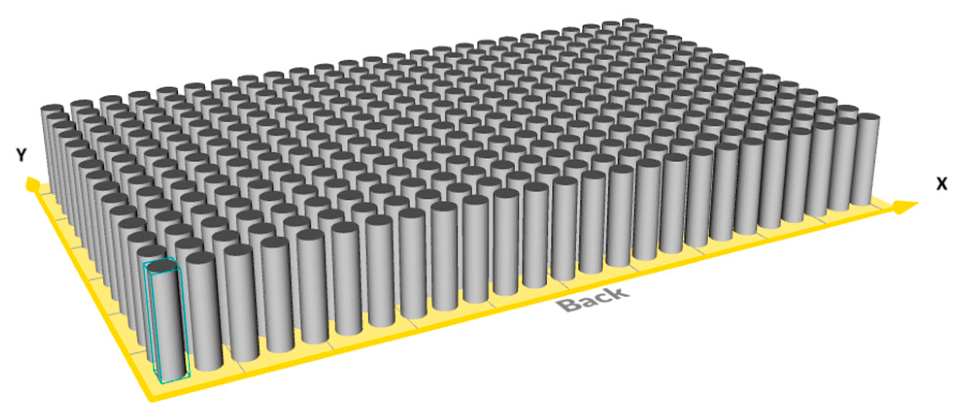
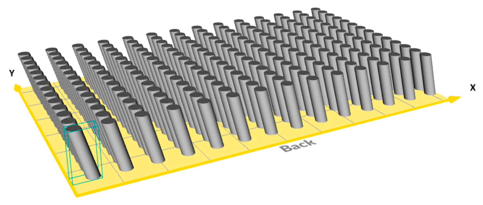
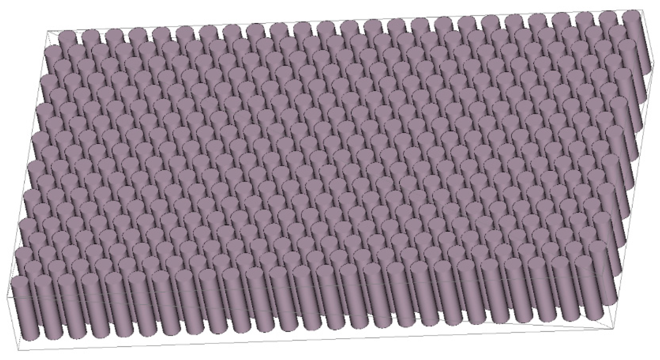
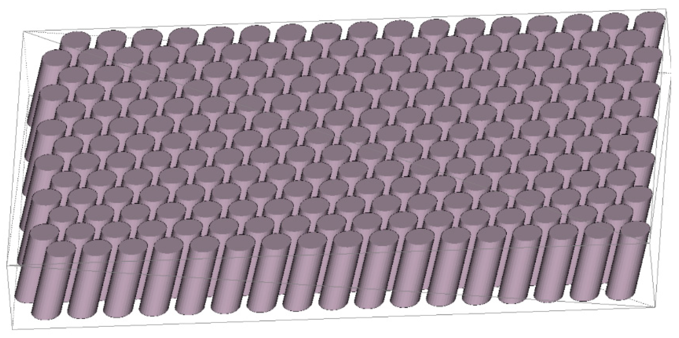
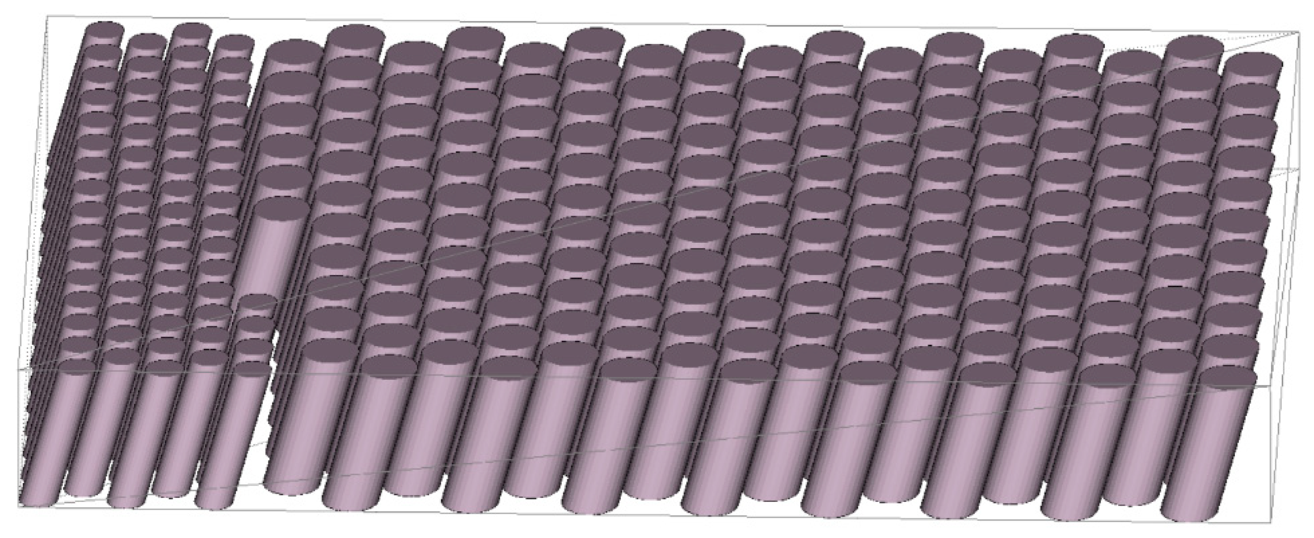
Figure 1. Process steps and relevant cost categories for AM of polymer and ceramic components.
Ceramics 06 00038 g001
Figure 2. Example for the automatically generated arrangement of three different cylinder geometries using the bounding box method.
Ceramics 06 00038 g002
Figure 3. Components (375 in number) of CG1 arranged on the building platform.
Ceramics 06 00038 g003
Figure 4. Components (196 in number) of CG2 arranged on the building platform.
Ceramics 06 00038 g004
Figure 5. Components (110 in number) of CG3 arranged on the building platform.
Ceramics 06 00038 g005
Figure 6. Components (64 in number) of each CGx arranged on the building platform (side view and top view).
Ceramics 06 00038 g006
Figure 7. An example of a lattice.
Ceramics 06 00038 g007
Figure 8. Adjusted quasi-phi-functions for appropriate geometries are used for describing non-overlapping of components with minimal allowable distances (left) and phi-functions are applied for containment of components in the cuboidal container (right).
Ceramics 06 00038 g008
Figure 9. Different types of regular packing of sections for the same geometry: (a) diagram of four types of sections; (b) examples of two types of sections for the same geometry.
Ceramics 06 00038 g009
Figure 10. Variants for the combination of two sections: (a) in terms of arrows a and s; (b) in terms of types of sections and geometries.
Ceramics 06 00038 g010
Figure 11. Combination of a pair of sections: (a) Section of Type 3 for Geometry 1; (b) Section of Type 3 for Geometry 2; (c) Combination of these two sections according to Variant 8.
Ceramics 06 00038 g011
Figure 12. Examples of combinations of two sections using “swap” technique: (a) cylinders of the same size but with different inclinations, (b) cylinders with the same inclinations but of different size.
Ceramics 06 00038 g012
Figure 13. Examples of sections assuming arrow a is parallel to Y-axis.
Ceramics 06 00038 g013
Figure 14. Examples of combinations of sections assuming each arrow a is parallel to Y-axis.
Ceramics 06 00038 g014
Figure 15. Arrangement of the CGx on BP_1_1-1.
Ceramics 06 00038 g015
Figure 16. Arrangement of the CGx on BP_1_2-1 and 1_3-1.
Ceramics 06 00038 g016
Figure 17. Arrangement of the CGx on BP_1_2-2 and 1_3-2.
Ceramics 06 00038 g017
Figure 18. Arrangement of the CGx on BP_1_2-3 and 1_3-3.
Ceramics 06 00038 g018
Figure 19. Arrangement of the CGx on BP_1_2-4 and 1_3-4.
Ceramics 06 00038 g019
Figure 20. Arrangement of the CGx on BP_1_2-5.
Ceramics 06 00038 g020
Figure 21. Arrangement of the CGx on BP_1_3-5.
Ceramics 06 00038 g021
Figure 22. Ceramic heat sinks (left and right) and static mixer (centered) manufactured at Fraunhofer IKTS via CerAM VPP with the CeraFab 7500 device and LithaLox 350 suspension of Lithoz.
Ceramics 06 00038 g022
Table 1. Parameters for the three types of cylinders for the illustration example.
Cylinder Geometry (CGx)CG1CG2CG3
length[mm]12.512.512.5
diameter[mm]334.5
inclination[°]01515
numbers needed (approx.)[1]100010001000
Table 2. Numbers of building platforms needed to manufacture approx. 1000 components of each cylinder geometry.
Numbers of CGx per Building PlatformNumber of Building Platforms Needed for approx. 1000 Components per Type
Kind of Building PlatformCG1CG2CG3
Max_CG1 (Figure E1)375 3|1125
Max_CG2 (Figure E2) 196 5|980
Max_CG3 (Figure E3) 1109|990
sum 17|1125 + 980 + 990
Equal_CGx (Figure E4)64646416|1024
Table 3. Numbers of different types of cylinder geometries (CG) arranged on the different building platforms for problem 1–solution 1.
Number of Building PlatformsNumbers of CGx per Building PlatformTotal Number of CGx
Kind of Building Platform CG1CG2CG3CG1CG2CG3
BP_1_1-19109109109981981981
10109109109109010901090
Table 4. Numbers of different types of cylinder geometries (CG) arranged on the different building platforms for problem 1–solution 2 with 988 components per type in nine printing jobs.
Number of Building PlatformsNumbers of CGx per Building PlatformTotal Number of CGx
Kind of Building Platform CG1CG2CG3CG1CG2CG3
BP_1_2-124500090000
BP_1_2-22040017080034
BP_1_2-340022100884
BP_1_2-4188188708818870
sum9 988988988
Table 5. Numbers of different types of cylinder geometries (CG) arranged on the different building platforms for problem 1–solution 3 with 1100 components per type in 10 printing jobs.
Number of Building PlatformsNumbers of CGx per Building PlatformTotal Number of CGx
Kind of Building Platform CG1CG2CG3CG1CG2CG3
BP_1_3-124500090000
BP_1_3-22040017080034
BP_1_3-340022100884
BP_1_3-4120023402002340
BP_1_3-51066182066182
sum10 110011001100
Disclaimer/Publisher’s Note: The statements, opinions and data contained in all publications are solely those of the individual author(s) and contributor(s) and not of MDPI and/or the editor(s). MDPI and/or the editor(s) disclaim responsibility for any injury to people or property resulting from any ideas, methods, instructions or products referred to in the content.

