
Using Low-Cost Radar Sensors and Action Cameras to Measure Inter-Vehicle Distances in Real-World Truck Platooning
 ,
,
Abstract
:1. Introduction
2. Materials and Methods
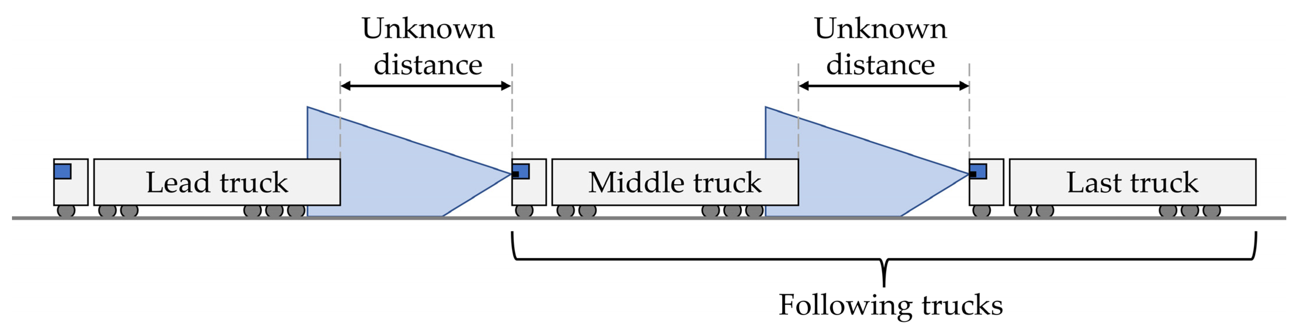
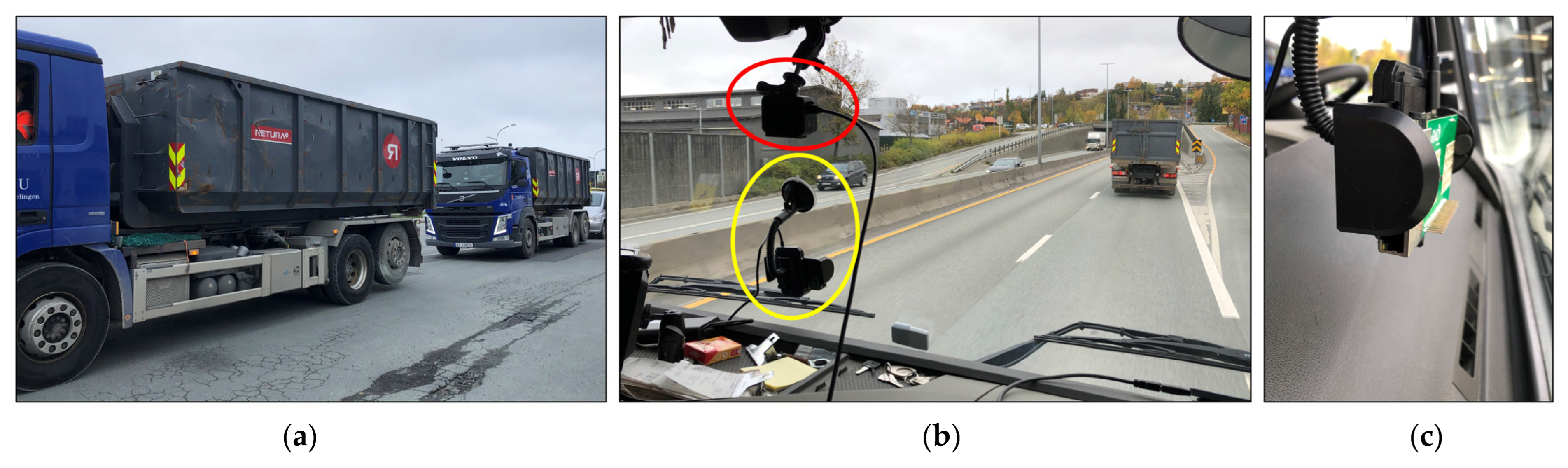
2.1. Data Collection Set-Up
2.2. Radar Sensors
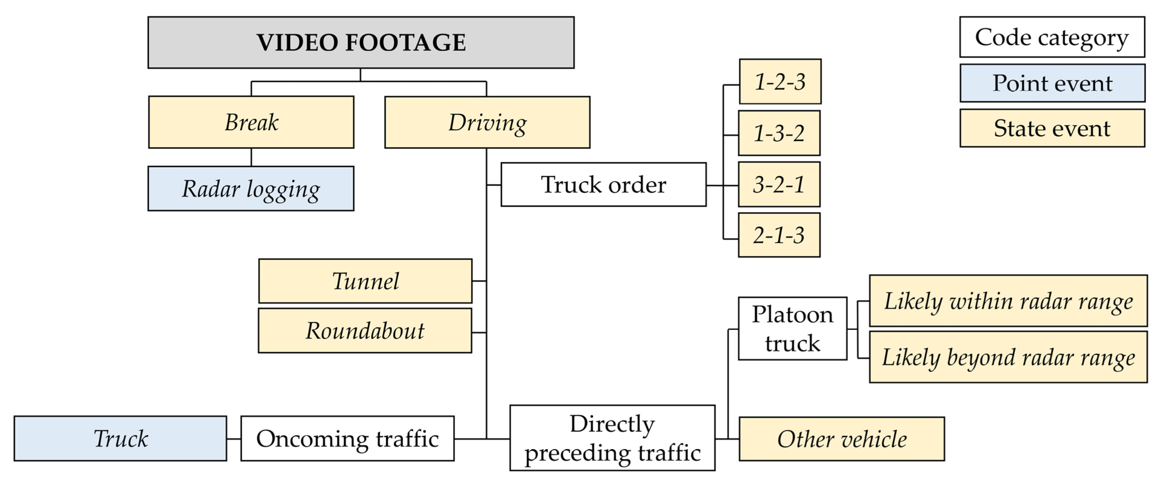
2.3. Video Footage, Synchronization and Manual Video Coding
2.4. Radar Data Processing
3. Results and Discussion
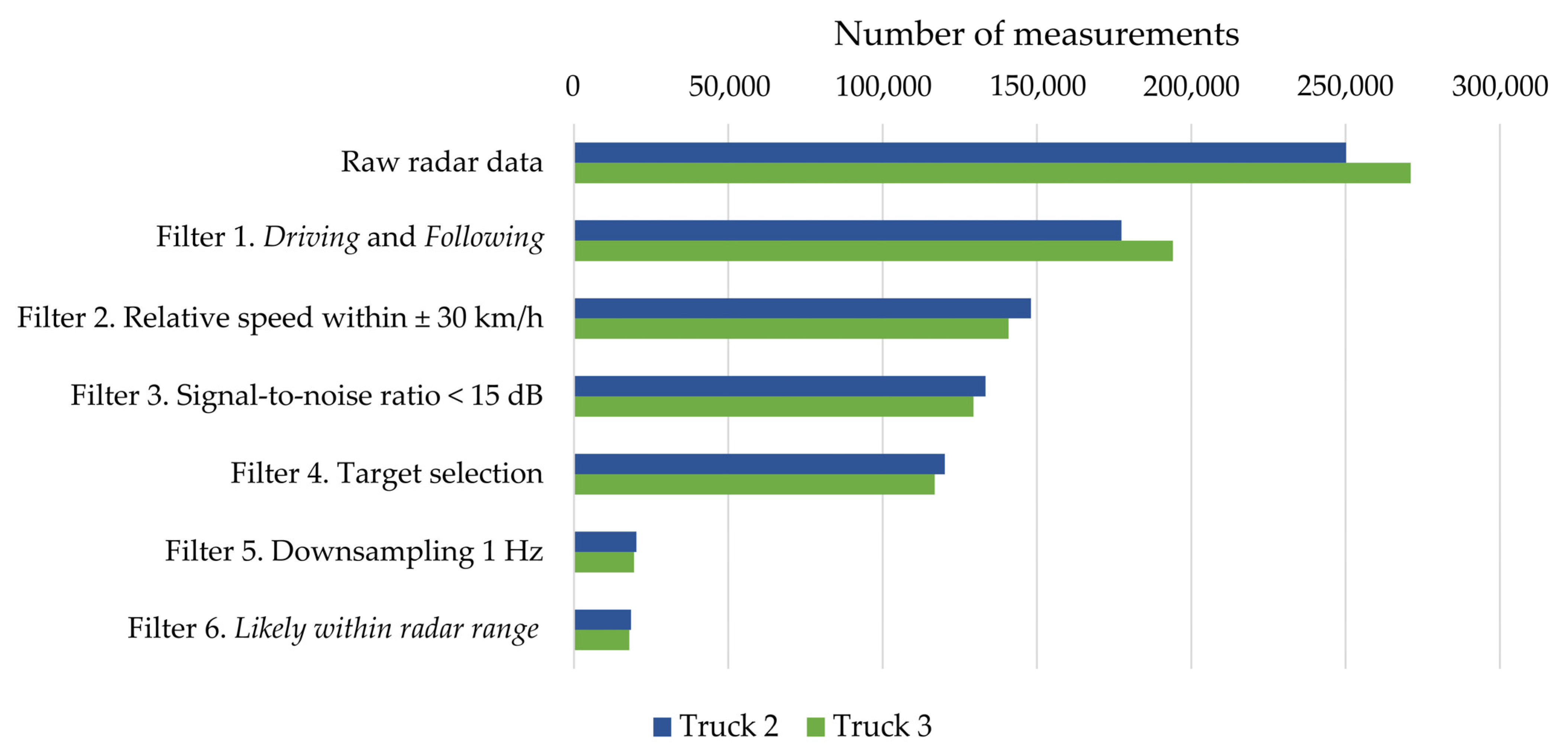
3.1. Impacts of Filtering
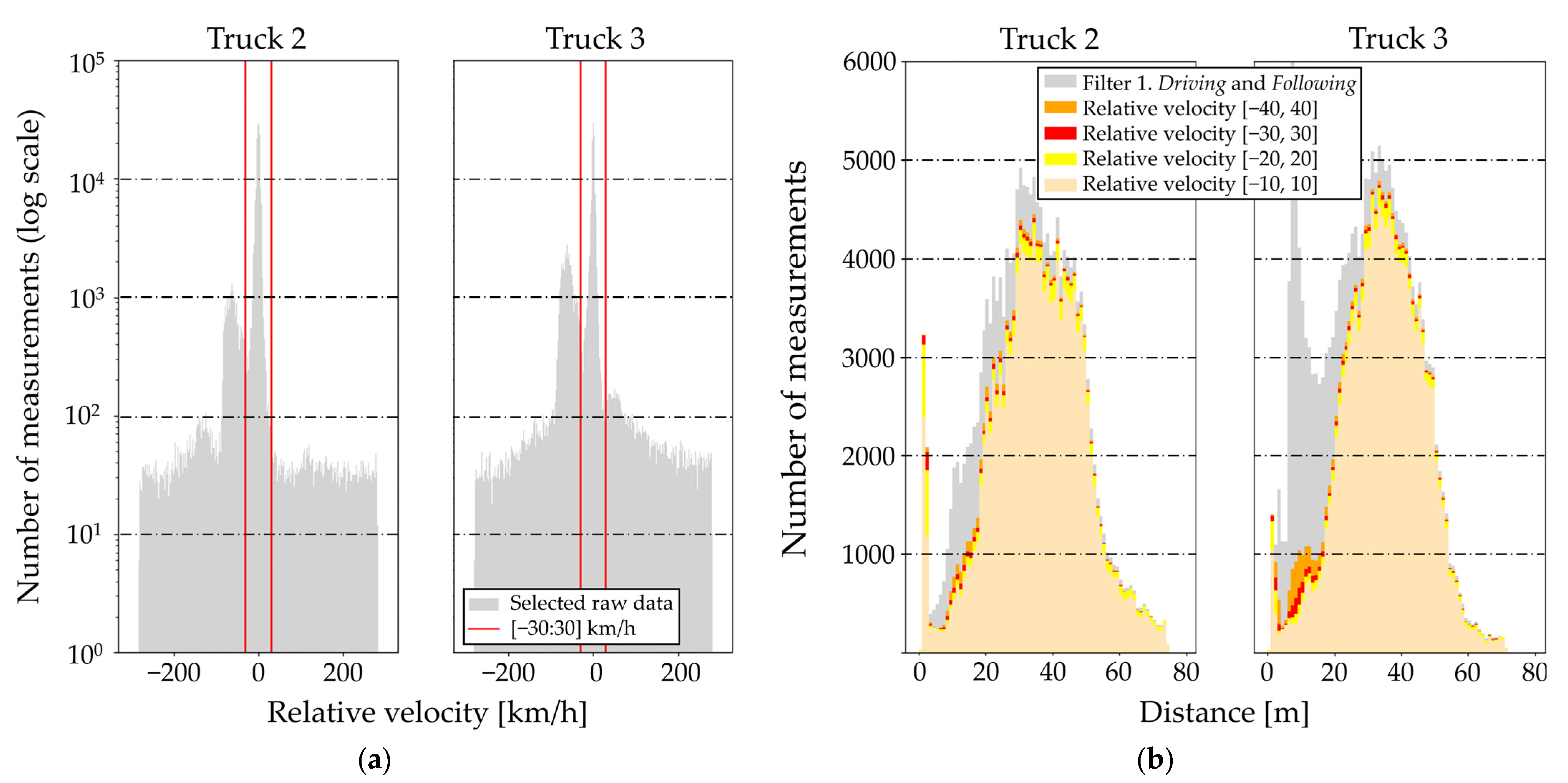
3.1.1. Relative Velocity
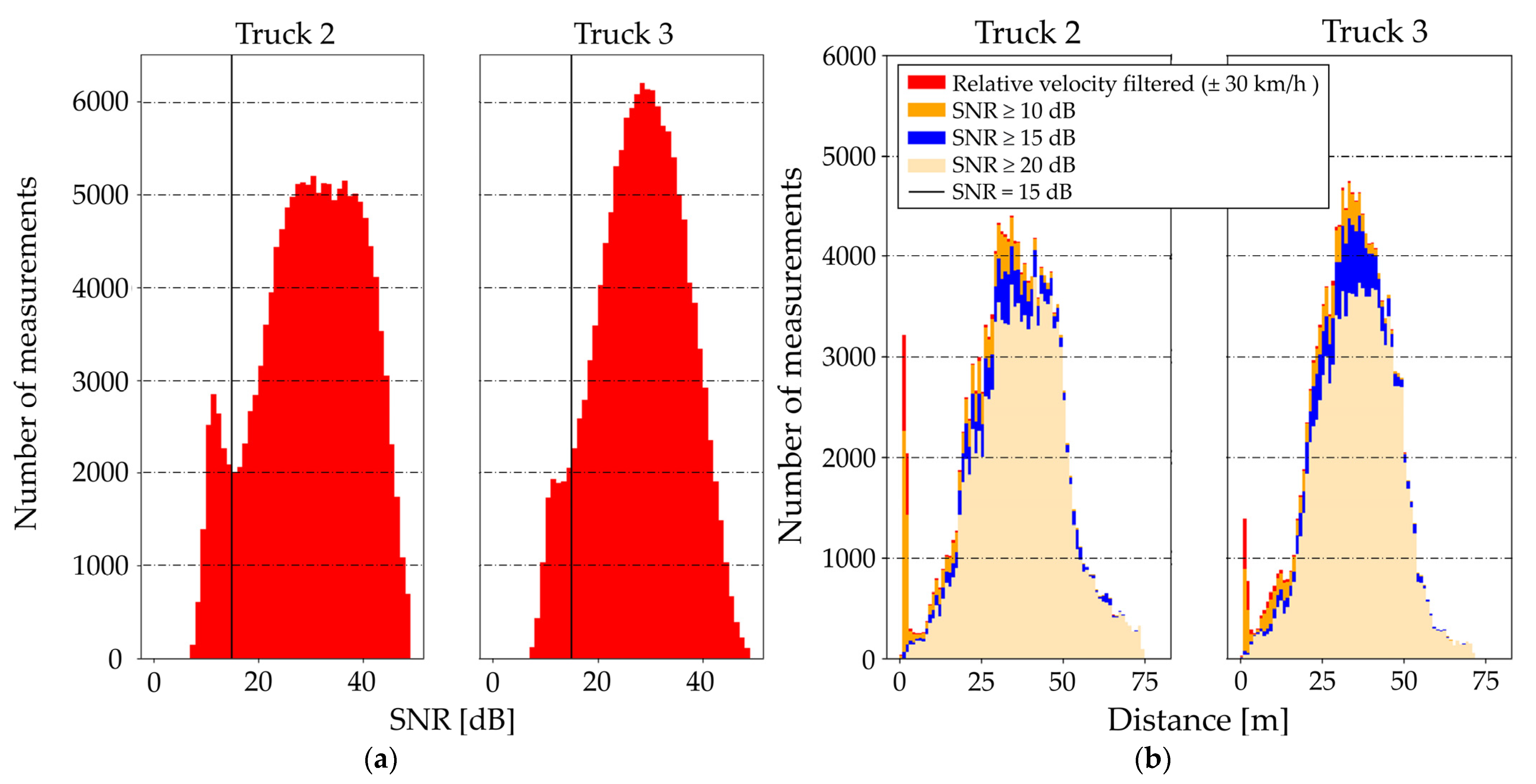
3.1.2. Signal-to Noise Ratio (SNR)
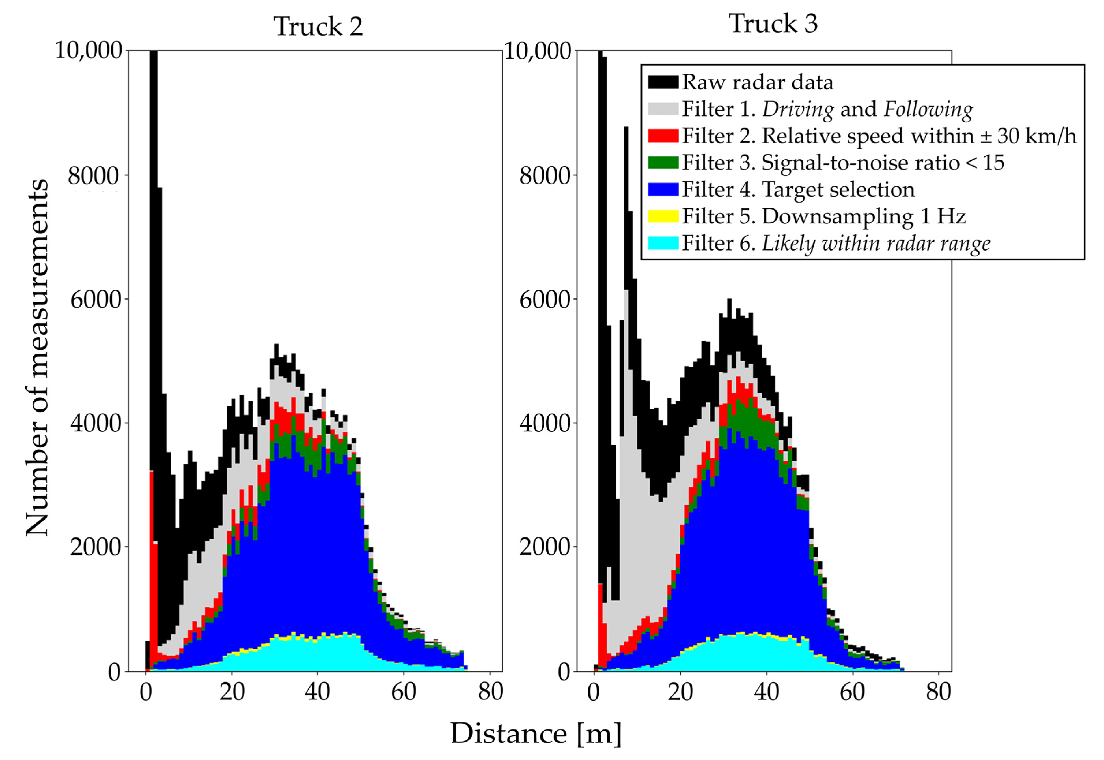
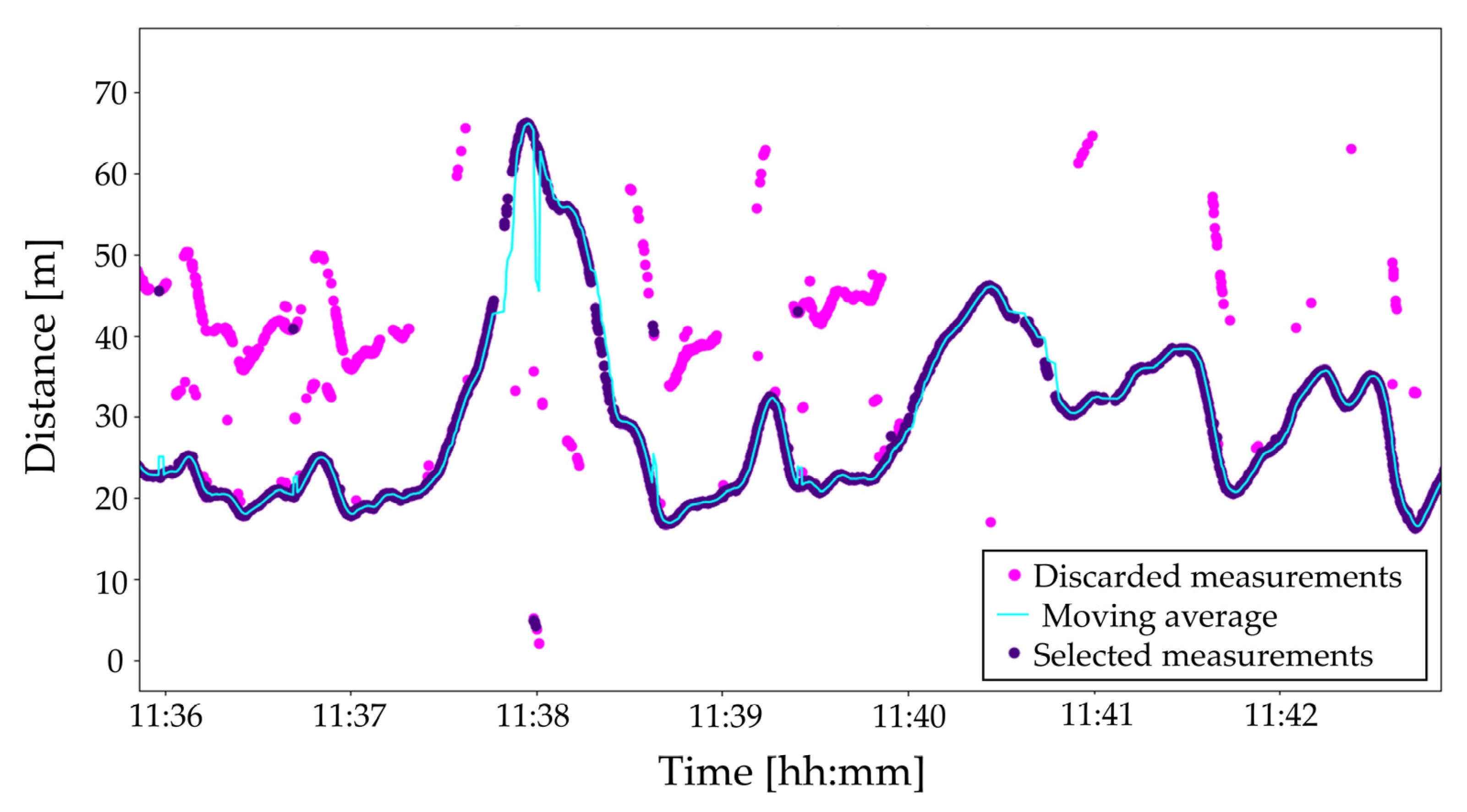
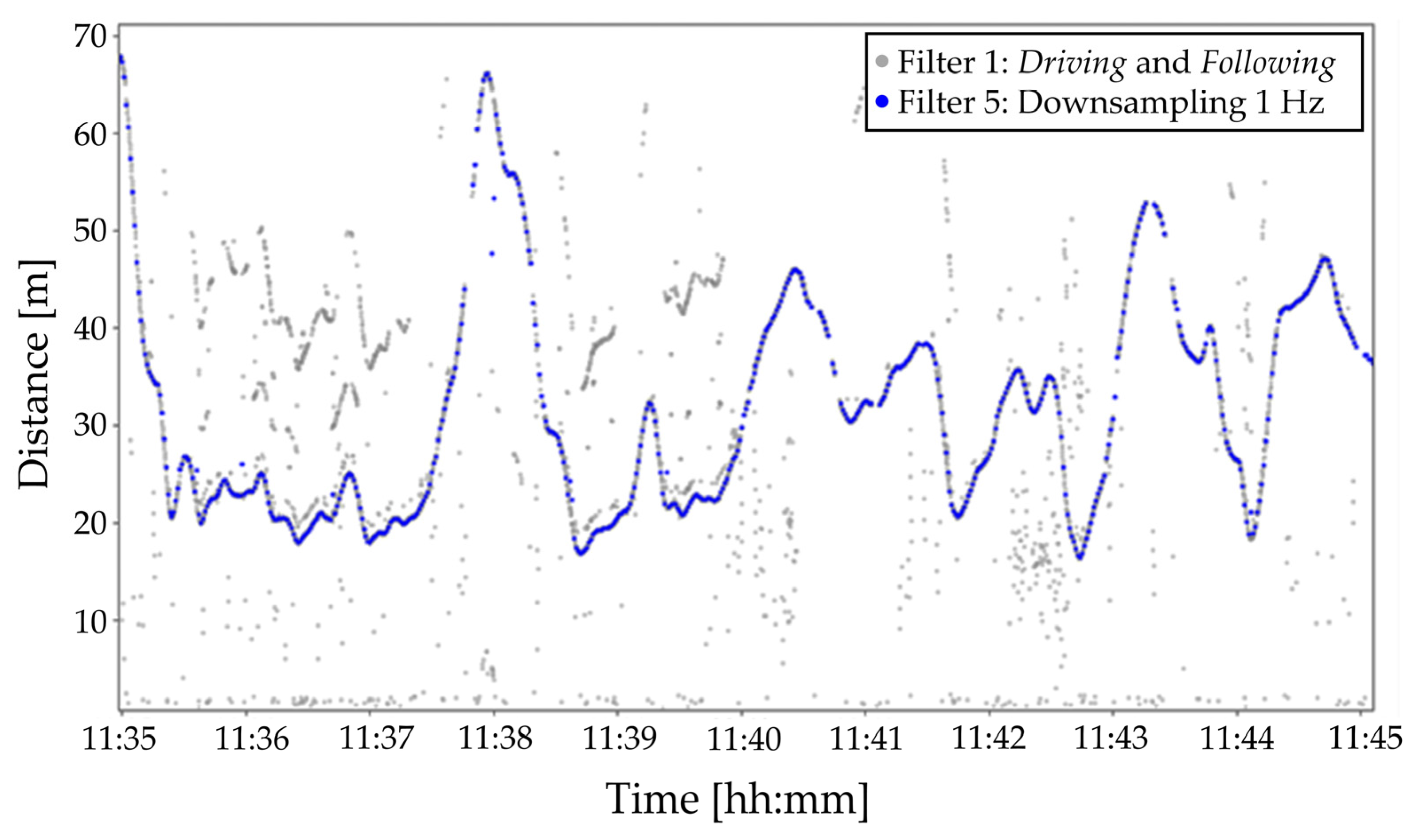
3.1.3. Distance
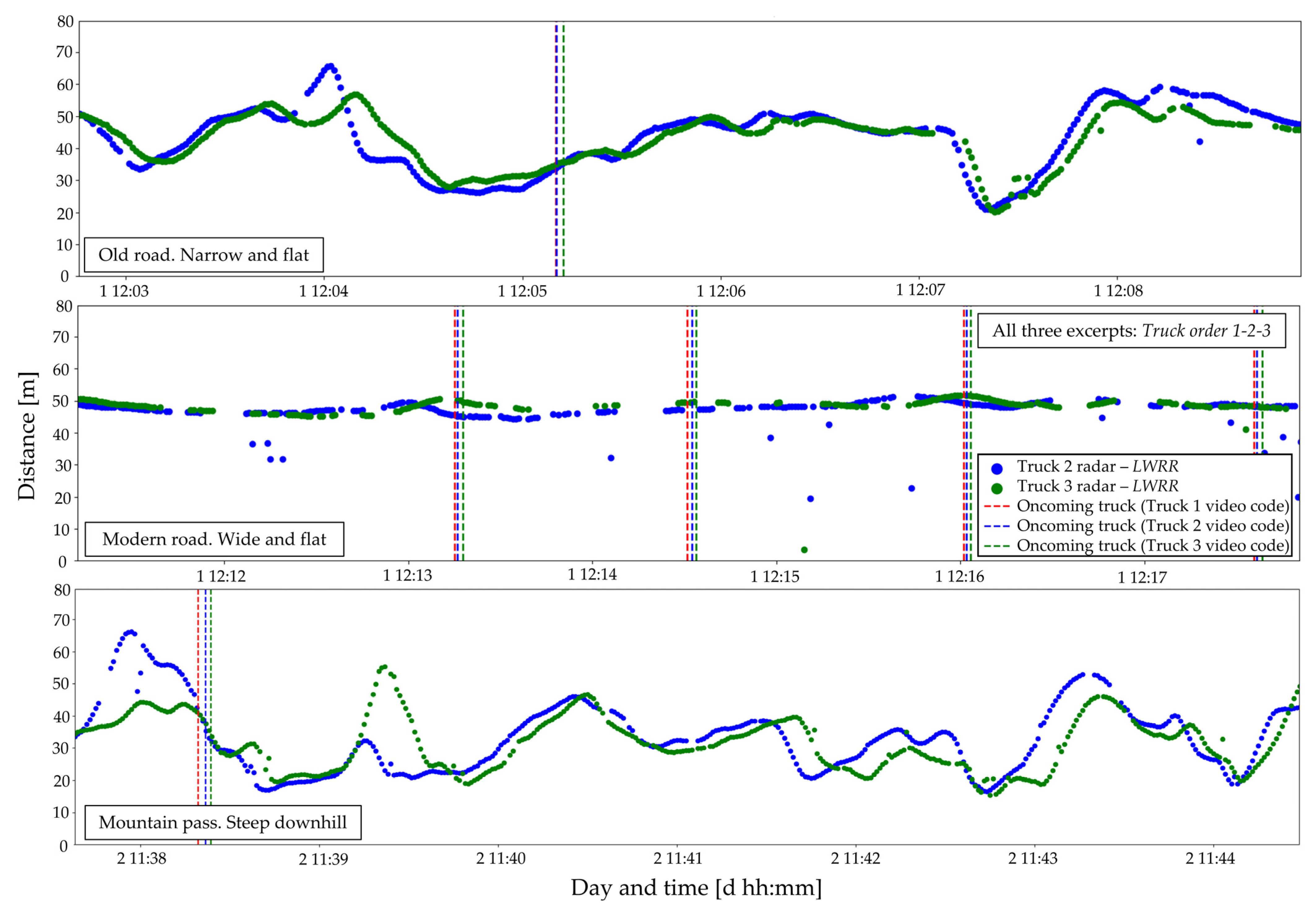
3.2. Radar Sensor Operation in Different Driving Situations
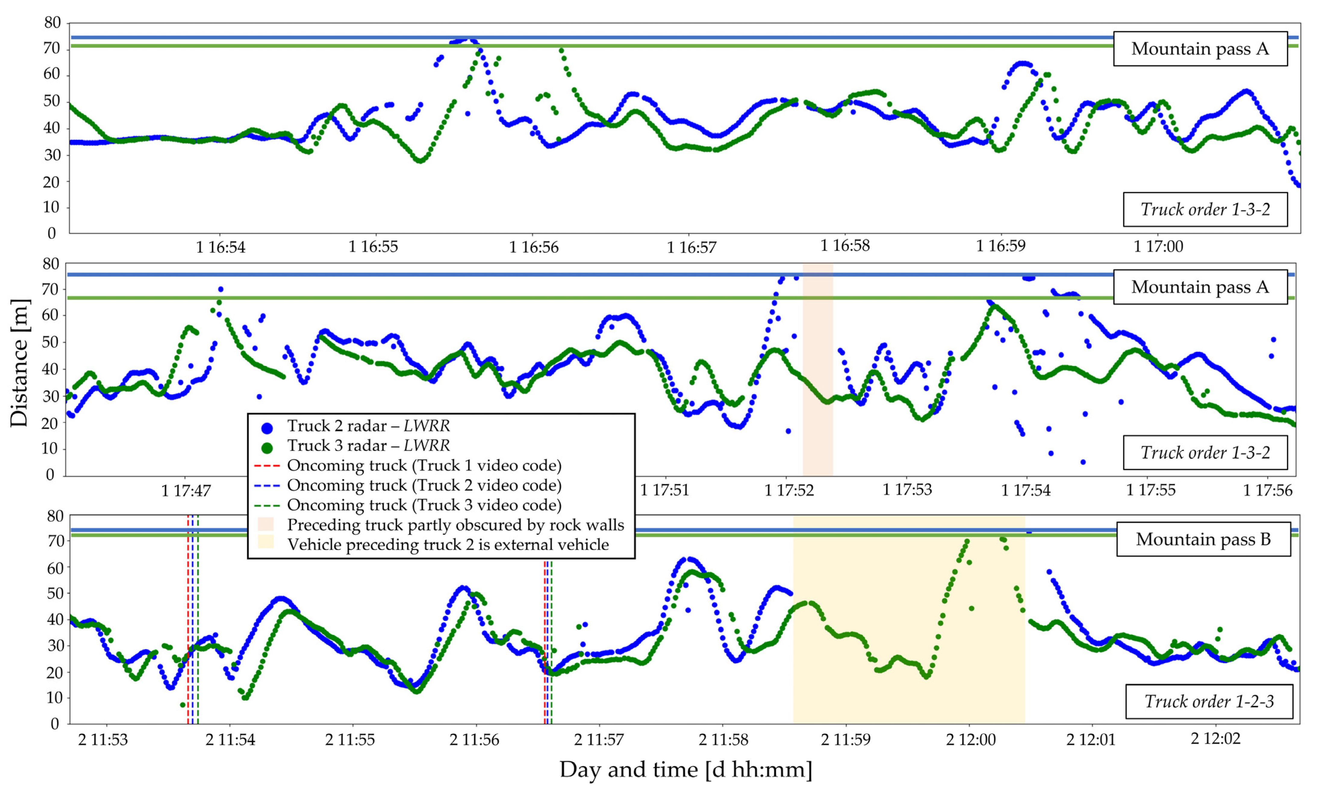
3.2.1. Visual Verification of Maximum Range
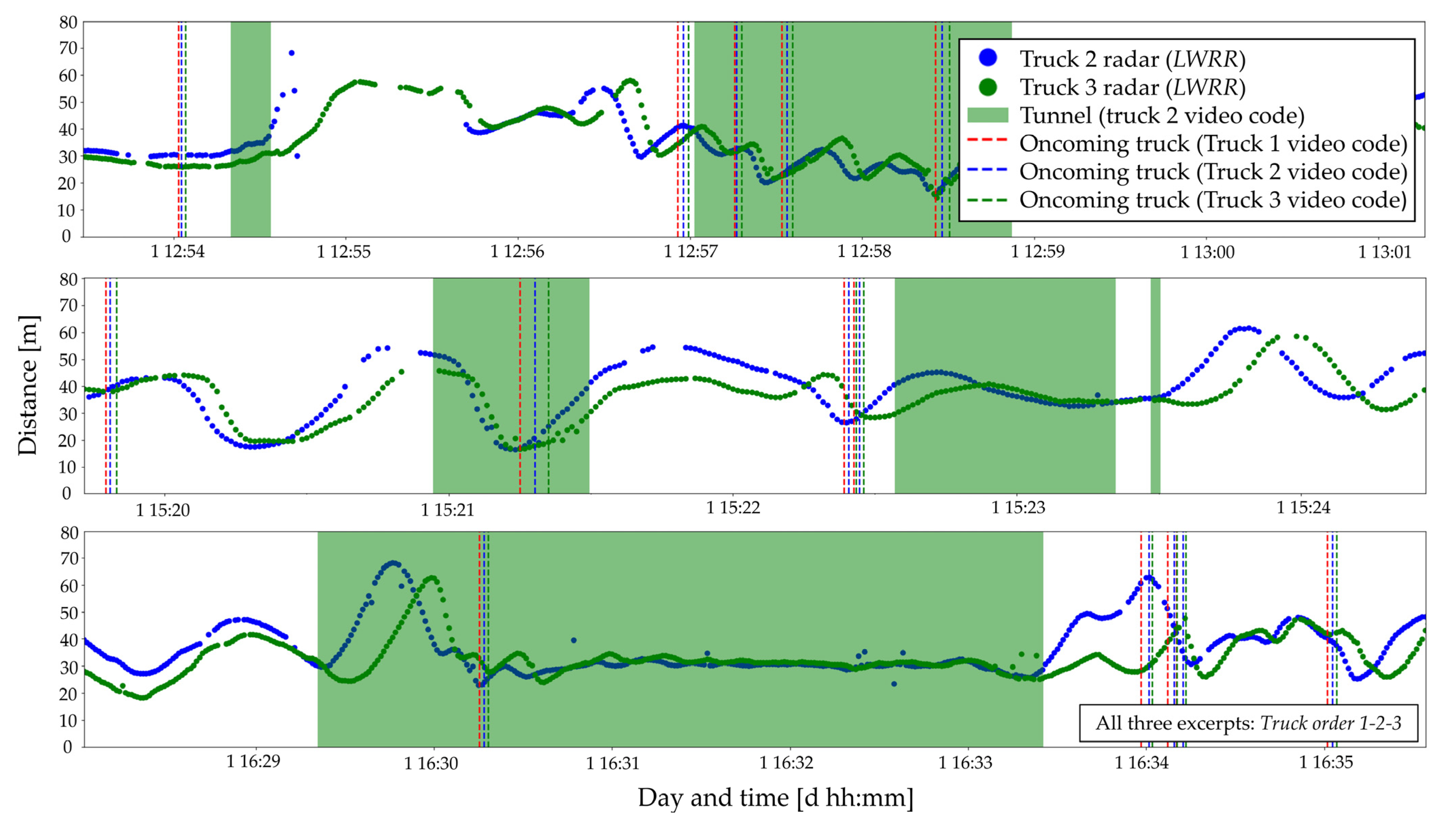
3.2.2. Tunnels
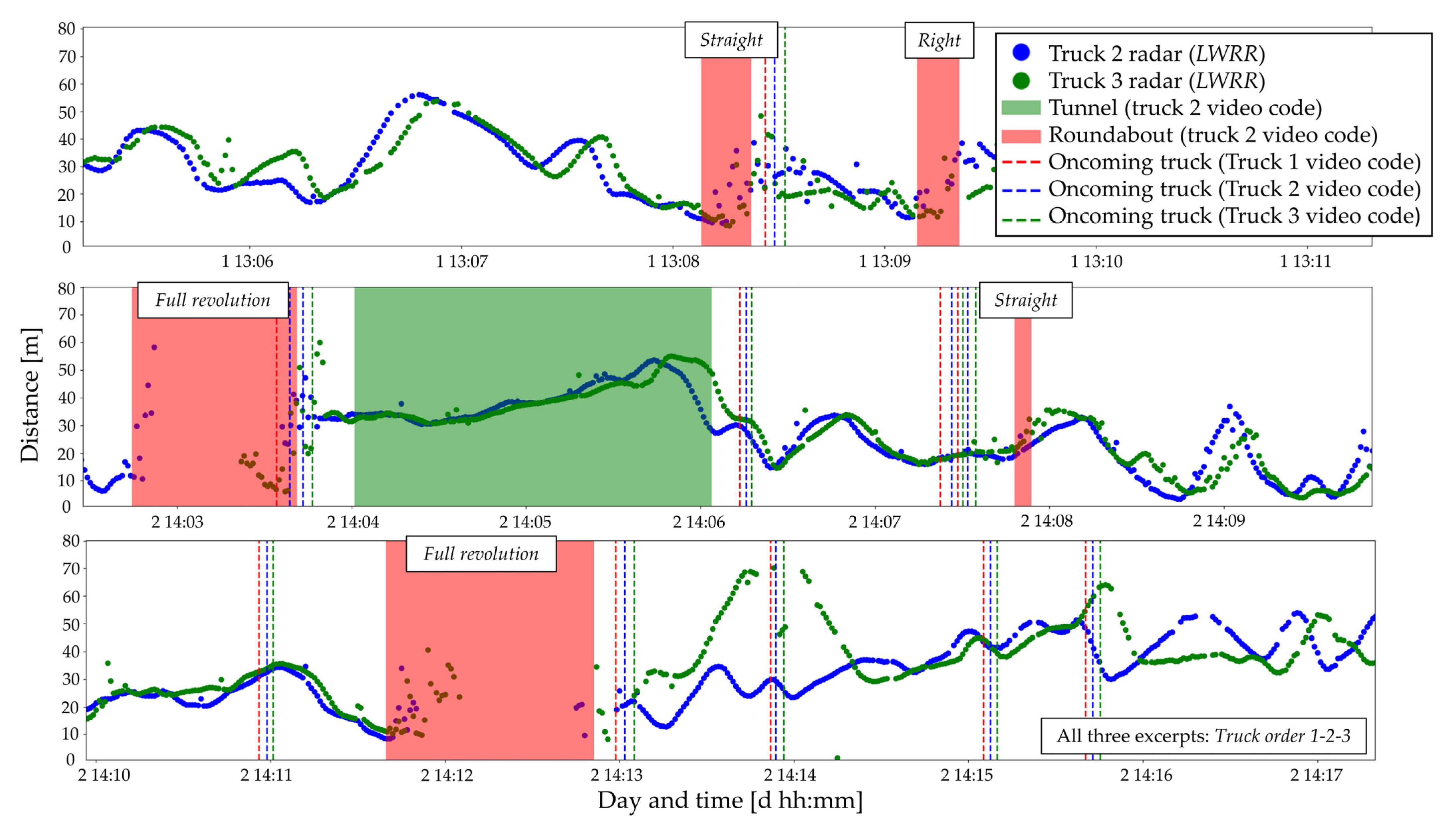
3.2.3. Roundabouts
3.3. Suggestions for Future Work
4. Conclusions
Author Contributions
Funding
Institutional Review Board Statement
Informed Consent Statement
Data Availability Statement
Acknowledgments
Conflicts of Interest
Appendix A
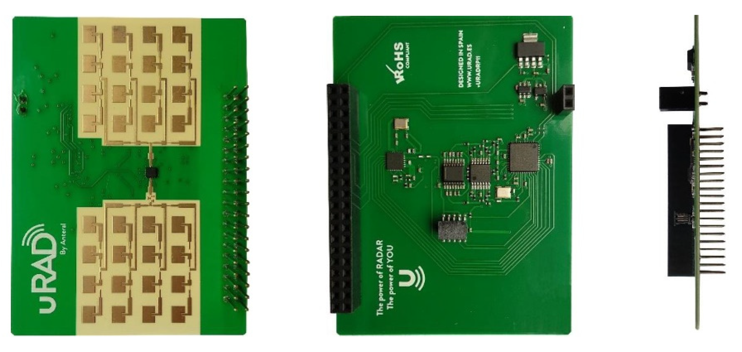
Appendix A.1. The Radar Sensors


| Parameter | Discussion |
|---|---|
| Mode | Of four modes available, only modes 3 (triangular) and 4 (dual-rate) measured both distance and velocity. Velocity would enable filtering away stationary and oncoming objects, to be left with desired inter-vehicle distance to the preceding truck. Modes 3 and 4 differed in upper distance range and update rate. Mode 3 had an upper distance range of 100 m, versus 75 m for mode 4. The supplier stated that the range would also depend on the target, meaning its radar cross-section: “(…) a person is detected up to 40 m. (…) a truck, that is bigger and reflects more, (…) will be detected [at] 70 m but probably (…) much farther. 100 m is not a limitation of the radar, [but] a guide (…) for very big targets.” Mode 4 should reduce ghost target detections in multi-target scenarios, at the expense of reduced range. |
| Ramp start freq., f0. Operation bandwidth, BW | Ramp start frequency, f0, could be set as 5–195 for modes 2–4. Operation bandwidth, BW, meaning the frequency sweep used in modes 2–4, depends on f0, and should be maximized, subject to Equation (A2), to increase accuracy and to distinguish closely located targets. For each radar, different values were chosen to avoid interference. |
| Samples and ramp duration, Ns | Ns is the number of samples taken from the reflected wave to calculate distance and velocity. Highest update rate requires lowest possible Ns. However, a trade-off is needed, since BW and Ns determine maximum range, through Equation (A3). |
| Max. detected targets, Ntar | Ntar is the number of targets that the sensor detects, 5 being maximum. If detecting more objects, the sensor logs data for those 5 with highest SNR. Ntar was maximized, capturing most data and providing possibility for filtering unwanted objects later. |
| Maximum detection distance, Rmax | For modes 2–4, Rmax is the maximum distance below which targets will be detected. Rmax artificially reduces the zone of interest, excluding targets beyond this distance, even if they have higher SNR than those within it. Rmax was chosen as 100 for all sensors, as this would search targets within the entire range. When asked if the sensors would stay fixed on the preceding truck in horizontal curves, the supplier stated that manual antenna modification could double the horizontal FOV, to the detriment of upper detection range. No manual modifications were made. For vertical curves, the supplier cited that the road in front of the truck, which would be more visible in vertical sag curves, could reflect the signal, masking the preceding truck. |
| Moving target indi-cator, MTI. Movement detection, Mth | Moving target indicator (MTI) allowed for including data only from objects with motion relative to the sensor. Mth is only relevant when using uRAD as a movement detector, and was not used. |
| Pre-Test Steps | Parameters | User Experience | Supplier Modifications and Recommendations |
|---|---|---|---|
1: Passenger car test with one radar sensor and standard graphical user interface (GUI) | Mode = 2 f0 = 45 BW = 200 Ns = 200 Ntar = 5 Rmax = 100 MTI = 1 Mth = 1 |
|
|
2: Test with two dump trucks. Follower with dashcam and one radar sensor | Mode = 2, 3 f0 = 45 BW = 200 Ns = 200 Ntar = 5 Rmax = 100 MTI = 1 Mth = 0 |
|
|
| Truck ID | Common Parameters | Specific Parameters |
|---|---|---|
| 2 | Mode = 3 BW = 200 MHz Ntar = 5 targets Rmax = 100 m MTI = 1 (active) Mth = 0 (inactive) | f0 = 5 MHz Ns = 200 samples |
| 3 | f0 = 25 MHz Ns = 195 samples |
Appendix A.2. Video Footage, Video Synchronization and Manual Video Coding
| Video Code | Definition |
|---|---|
| Driving (S) | Driving starts when the truck is fully inside the correct lane on the roadway, with the steering wheel turned straight. It stops just before the driver starts turning the wheel, with the intention of entering driveways, parking areas or stop pockets. Except during Break and periods of camera malfunctions, every other video code is coded only when Driving is also active. |
| Break (S) | All time that is not Driving, is defined as Break. This includes maneuvering in and out of driveways, parking areas and stop pockets. |
| Event | Illustrations |
|---|---|
| Tunnel |   |
| Roundabout (Left): Straight; (Right) Right-turn |   |
| LWRR (likely within radar range) |   |
| LBRR (likely beyond radar range) |   |
Appendix A.3. Radar Data Curation


Appendix A.4. Results and Discussion
| Filtering Step | Truck Number | |||||||
|---|---|---|---|---|---|---|---|---|
| 2 | 3 | |||||||
| Min | Avg | Max | Std | Min | Avg | Max | Std | |
| Raw | −280.9 | −5.7 | 281.0 | 40.4 | −280.7 | −9.4 | 280.7 | 45.9 |
| 1 | −280.9 | −7.7 | 281.0 | 43.7 | −280.7 | −11.3 | 280.7 | 48.9 |
| 2 | −29.9 | −0.5 | 29.9 | 5.5 | −29.9 | −0.5 | 29.9 | 5.5 |
| 3 | −29.9 | −0.3 | 29.9 | 4.8 | −29.9 | −0.3 | 29.7 | 4.6 |
| 4 | −29.9 | −0.2 | 29.9 | 4.4 | −29.9 | −0.2 | 29.7 | 4.2 |
| 5 | −29.6 | −0.2 | 28.6 | 4.3 | −29.9 | −0.2 | 27.2 | 4.0 |
| 6 | −29.6 | −0.1 | 28.6 | 4.2 | −29.7 | −0.1 | 27.2 | 3.8 |
| Filtering Step | Truck Number | |||||||
|---|---|---|---|---|---|---|---|---|
| 2 | 3 | |||||||
| Min | Avg | Max | Std | Min | Avg | Max | Std | |
| Raw | 6.8 | 24.6 | 53.9 | 10.8 | 6.6 | 22.6 | 51.4 | 9.7 |
| 1 | 6.9 | 27.6 | 53.9 | 10.6 | 6.7 | 24.2 | 51.4 | 9.9 |
| 2 | 6.9 | 29.9 | 53.9 | 9.9 | 6.8 | 28.1 | 51.4 | 8.5 |
| 3 | 15.1 | 31.8 | 53.9 | 8.3 | 15.1 | 29.5 | 51.4 | 7.3 |
| 4 | 15.1 | 32.9 | 53.9 | 7.9 | 15.1 | 30.4 | 51.4 | 7.0 |
| 5 | 15.1 | 31.6 | 49.7 | 6.9 | 15.1 | 29.4 | 47.7 | 5.9 |
| 6 | 15.1 | 31.8 | 49.7 | 6.9 | 15.1 | 29.5 | 47.7 | 5.8 |
| Distance Bins | Avg. Relative Velocity (km/h) | Average SNR (dB) | # Measurements | % of Total |
|---|---|---|---|---|
| 0–10 | −0.4 | 30.0 | 204 | 1% |
| 10–20 | −1.0 | 32.3 | 1191 | 6% |
| 20–30 | −0.3 | 31.1 | 3327 | 18% |
| 30–40 | −0.1 | 31.8 | 5074 | 27% |
| 40–50 | 0.0 | 32.4 | 5519 | 30% |
| 50–60 | 0.2 | 31.4 | 2151 | 12% |
| 60–70 | −0.1 | 31.2 | 813 | 4% |
| 70+ | 0.7 | 32.2 | 191 | 1% |
| Distance Bins | Avg. Relative Velocity (km/h) | Average SNR (dB) | # Measurements | % of Total |
|---|---|---|---|---|
| 0–10 | −0.3 | 29.4 | 199 | 1% |
| 10–20 | −1.2 | 29.1 | 1113 | 6% |
| 20–30 | −0.4 | 28.6 | 4173 | 23% |
| 30–40 | 0.0 | 29.0 | 5642 | 31% |
| 40–50 | 0.1 | 30.2 | 4988 | 28% |
| 50–60 | 0.0 | 31.0 | 1502 | 8% |
| 60–70 | 0.9 | 31.6 | 270 | 2% |
| 70+ | 0.4 | 31.4 | 29 | 0% |
| Truck | Relative Velocity | |||
|---|---|---|---|---|
| Avg | Min | Max | Std | |
| 2 | 0.1 | −19.7 | 28.6 | 3.5 |
| 3 | 0.1 | −19.3 | 18.8 | 3.3 |
| Truck | Distance | SNR | ||||||
|---|---|---|---|---|---|---|---|---|
| Avg | Min | Max | Std | Avg | Min | Max | Std | |
| 2 | 36.4 | 10.6 | 68.2 | 10.5 | 30.8 | 15.1 | 46.9 | 6.4 |
| 3 | 36.2 | 13.8 | 65.0 | 9.6 | 28.5 | 15.7 | 44.0 | 5.2 |
| Truck | Distance | SNR | ||||||
|---|---|---|---|---|---|---|---|---|
| Avg | Min | Max | Std | Avg | Min | Max | Std | |
| 2 | 23.3 | 8.6 | 58.4 | 10.1 | 24.5 | 16.2 | 39.5 | 5.2 |
| 3 | 22.4 | 6.3 | 60.0 | 11.2 | 22.4 | 15.1 | 41.5 | 4.4 |
| Truck | Relative Velocity | |||
|---|---|---|---|---|
| Avg | Min | Max | Std | |
| 2 | −6.5 | −27.8 | 11.2 | 9.1 |
| 3 | −5.9 | −25.7 | 10.5 | 8.9 |
References
- Tsugawa, S.; Jeschke, S.; Shladover, S.E. A Review of Truck Platooning Projects for Energy Savings. IEEE Trans. Intell. Veh. 2016, 1, 68–77. [Google Scholar] [CrossRef]
- Eitrheim, M.H.R.; Log, M.M.; Tørset, T.; Levin, T.; Pitera, K. Opportunities and Barriers for Truck Platooning on Norwegian Rural Freight Routes. Transp. Res. Rec. 2022, 2676, 810–824. [Google Scholar] [CrossRef]
- Horenberg, D. Applications within Logistics 4.0: A Research Conducted on the Visions of 3PL Service Providers. In Proceedings of the 9th IBA Bachelor Thesis Conference; University of Twente, The Faculty of Behavioural, Management and Social Sciences: Enschede, The Netherlands, 2017. [Google Scholar]
- Bergenhem, C.; Shladover, S.; Coelingh, E.; Englund, C.; Tsugawa, S. Overview of Platooning Systems. In Proceedings of the 19th ITS World Congress, Vienna, Austria, 22–26 October 2012. [Google Scholar]
- Konstantinopoulou, L.; Coda, A.; Schmidt, F. Specifications for Multi-Brand Truck Platooning. In Proceedings of the 8th International Conference on Weigh-In-Motion, Prague, Czech Republic, 20–23 May 2019. [Google Scholar]
- Borealis. Available online: https://www.vegvesen.no/vegprosjekter/europaveg/e8borealis/ (accessed on 1 March 2023).
- Simonsen, J. Ground-Breaking EU Project on Automated Heavy-Haul Freight Vehicles to Be Launched. ITS Norway: Oslo, Norway. Press Release, 1 October 2022. Available online: https://its-norway.no/ground-breaking-eu-project-on-automated-heavy-haul-freight-vehicles-to-be-launched/ (accessed on 3 January 2023).
- Robinson, T.; Coelingh, E. Operating Platoons On Public Motorways: An Introduction To The SARTRE Platooning Programme. In Proceedings of the 17th World Congress on Intelligent Transport Systems, Busan, Republic of Korea, 25–29 October 2010. [Google Scholar]
- Zhang, L.; Chen, F.; Ma, X.; Pan, X. Fuel Economy in Truck Platooning: A Literature Overview and Directions for Future Research. J. Adv. Transp. 2020, 2020, e2604012. [Google Scholar] [CrossRef]
- Srisomboon, I.; Lee, S. Efficient Position Change Algorithms for Prolonging Driving Range of a Truck Platoon. Appl. Sci. 2021, 11, 10516. [Google Scholar] [CrossRef]
- Hakobyan, G.; Yang, B. High-Performance Automotive Radar: A Review of Signal Processing Algorithms and Modulation Schemes. IEEE Signal Process. Mag. 2019, 36, 32–44. [Google Scholar] [CrossRef]
- Scheiner, N.; Kraus, F.; Appenrodt, N.; Dickmann, J.; Sick, B. Object Detection for Automotive Radar Point Clouds—A Comparison. AI Perspect. 2021, 3, 6. [Google Scholar] [CrossRef]
- Ju, Y.; Jin, Y.; Lee, J. Design and Implementation of a 24 GHz FMCW Radar System for Automotive Applications. In Proceedings of the 2014 International Radar Conference, Lille, France, 13–17 October 2014; pp. 1–4. [Google Scholar]
- Venon, A.; Dupuis, Y.; Vasseur, P.; Merriaux, P. Millimeter Wave FMCW RADARs for Perception, Recognition and Localization in Automotive Applications: A Survey. IEEE Trans. Intell. Veh. 2022, 7, 533–555. [Google Scholar] [CrossRef]
- Bilik, I.; Longman, O.; Villeval, S.; Tabrikian, J. The Rise of Radar for Autonomous Vehicles: Signal Processing Solutions and Future Research Directions. IEEE Signal Process. Mag. 2019, 36, 20–31. [Google Scholar] [CrossRef]
- Shnidman, D.A. Radar Detection in Clutter. IEEE Trans. Aerosp. Electron. Syst. 2005, 41, 1056–1067. [Google Scholar] [CrossRef]
- Wang, L.; Giebenhain, S.; Anklam, C.; Goldluecke, B. Radar Ghost Target Detection via Multimodal Transformers. IEEE Robot. Autom. Lett. 2021, 6, 7758–7765. [Google Scholar] [CrossRef]
- Ortiz, F.M.; Sammarco, M.; Costa, L.H.M.K.; Detyniecki, M. Applications and Services Using Vehicular Exteroceptive Sensors: A Survey. IEEE Trans. Intell. Veh. 2023, 8, 949–969. [Google Scholar] [CrossRef]
- Gu, Y.; Hsu, L.-T.; Kamijo, S. Passive Sensor Integration for Vehicle Self-Localization in Urban Traffic Environment. Sensors 2015, 15, 30199–30220. [Google Scholar] [CrossRef] [PubMed]
- Wang, F.; Zhuang, W.; Yin, G.; Liu, S.; Liu, Y.; Dong, H. Robust Inter-Vehicle Distance Measurement Using Cooperative Vehicle Localization. Sensors 2021, 21, 2048. [Google Scholar] [CrossRef] [PubMed]
- Kim, T.-W.; Jang, W.-S.; Jang, J.; Kim, J.-C. Camera and Radar-Based Perception System for Truck Platooning. In Proceedings of the 2020 20th International Conference on Control, Automation and Systems (ICCAS), Busan, Republic of Korea, 13–16 October 2020; pp. 950–955. [Google Scholar]
- URAD Radar for Raspberry Pi. Available online: https://urad.es/en/product/urad-radar-raspberry-pi/ (accessed on 26 January 2023).
- Eitrheim, M.H.R.; Log, M.M.; Tørset, T.; Levin, T.; Nordfjærn, T. Driver Workload in Truck Platooning: Insights from an on-Road Pilot Study on Rural Roads. In Proceedings of the 32nd European Safety and Reliability Conference (ESREL 2022), Dublin, Ireland, 28 August–1 September 2022. [Google Scholar]
- Knoop, V.L.; Wang, M.; Wilmink, I.; Hoedemaeker, D.M.; Maaskant, M.; Van der Meer, E.-J. Platoon of SAE Level-2 Automated Vehicles on Public Roads: Setup, Traffic Interactions, and Stability. Transp. Res. Rec. 2019, 2673, 311–322. [Google Scholar] [CrossRef]
- Mills, D.L. Internet Time Synchronization: The Network Time Protocol. IEEE Trans. Commun. 1991, 39, 1482–1493. [Google Scholar] [CrossRef]
- Emerald Sequoia LLC Emerald Time. Available online: https://emeraldsequoia.com/et/ (accessed on 27 January 2023).
- Racelogic 04—VBOX Sport Logging. Available online: https://en.racelogic.support/VBOX_Motorsport/Product_Info/Performance_Meters/VBOX__Sport/VBOX_Sport_User_Guide/04_-_VBOX_Sport_Logging (accessed on 8 March 2023).
- Rohling, H.; Meinecke, M.-M. Waveform Design Principles for Automotive Radar Systems. In Proceedings of the 2001 CIE International Conference on Radar Proceedings (Cat No.01TH8559), Beijing, China, 15–18 October 2001; pp. 1–4. [Google Scholar]
- Al-Hasan, T.M.; Shibeika, A.S.; Attique, U.; Bensaali, F.; Himeur, Y. Smart Speed Camera Based on Automatic Number Plate Recognition for Residential Compounds and Institutions Inside Qatar. In Proceedings of the 2022 5th International Conference on Signal Processing and Information Security (ICSPIS), Dubai, United Arab Emirates, 7–8 December 2022; pp. 42–45. [Google Scholar]
- Murad, M.; Bilik, I.; Friesen, M.; Nickolaou, J.; Salinger, J.; Geary, K.; Colburn, J.S. Requirements for next Generation Automotive Radars. In Proceedings of the 2013 IEEE Radar Conference (RadarCon13), Ottawa, ON, Canada, 29 April–3 May 2013; pp. 1–6. [Google Scholar]
- Ouaknine, A.; Newson, A.; Rebut, J.; Tupin, F.; Pérez, P. CARRADA Dataset: Camera and Automotive Radar with Range- Angle- Doppler Annotations. In Proceedings of the 2020 25th International Conference on Pattern Recognition (ICPR), Milan, Italy, 10–15 January 2021; pp. 5068–5075. [Google Scholar]
- Radhityo Sardjono, D.; Suratman, F.Y. Istiqomah Human Motion Change Detection Based On FMCW Radar. In Proceedings of the 2022 IEEE Asia Pacific Conference on Wireless and Mobile (APWiMob), Bandung, Indonesia, 9–10 December 2022; pp. 1–6. [Google Scholar]
- Erdyarahman, R.; Suratman, F.Y.; Pramudita, A.A. Contactless Human Respiratory Frequency Monitoring System Based on FMCW Radar. In Proceedings of the 2022 IEEE Asia Pacific Conference on Wireless and Mobile (APWiMob), Bandung, Indonesia, 9–10 December 2022; pp. 1–7. [Google Scholar]
- Oberhammer, J.; Somjit, N.; Shah, U.; Baghchehsaraei, Z. 16—RF MEMS for Automotive Radar. In Handbook of Mems for Wireless and Mobile Applications; Uttamchandani, D., Ed.; Woodhead Publishing Series in Electronic and Optical Materials; Woodhead Publishing: Sawston, UK, 2013; pp. 518–549. ISBN 978-0-85709-271-7. [Google Scholar]
- Friard, O.; Gamba, M. BORIS: A Free, Versatile Open-Source Event-Logging Software for Video/Audio Coding and Live Observations. Methods Ecol. Evol. 2016, 7, 1325–1330. [Google Scholar] [CrossRef]
- Norwegian Public Roads Administration (NPRA) Handbook N302 Road Markings. Available online: https://viewers.vegnorm.vegvesen.no/product/859926/nb#id-8d46a74b-9c46-4790-b012-974ebf080aed (accessed on 20 February 2023).
- Suzuki, H.; Nakatsuji, T. Dynamic Estimation of Headway Distance in Vehicle Platoon System under Unexpected Car-Following Situations. Transp. Res. Procedia 2015, 6, 172–188. [Google Scholar] [CrossRef]
- Kim, T.; Park, T.-H. Extended Kalman Filter (EKF) Design for Vehicle Position Tracking Using Reliability Function of Radar and Lidar. Sensors 2020, 20, 4126. [Google Scholar] [CrossRef] [PubMed]
- Jing, L.; Yanping, Z.; Xingang, Z. On the Maximum Unambiguous Range of LFMCW Radar. In Proceedings of the 2019 International Conference on Information Technology and Computer Application (ITCA), Guangzhou, China, 20–22 December 2019; pp. 92–94. [Google Scholar]
- Berthold, P.; Michaelis, M.; Luettel, T.; Meissner, D.; Wuensche, H.-J. Radar Reflection Characteristics of Vehicles for Contour and Feature Estimation. In Proceedings of the 2017 Sensor Data Fusion: Trends, Solutions, Applications (SDF), Bonn, Germany, 10–12 October 2017; pp. 1–6. [Google Scholar]
- Macaveiu, A.; Câmpeanu, A. Automotive Radar Target Tracking by Kalman Filtering. In Proceedings of the 2013 11th International Conference on Telecommunications in Modern Satellite, Cable and Broadcasting Services (℡SIKS), Nis, Serbia, 16–19 October 2013; Volume 2, pp. 553–556. [Google Scholar]
- Folster, F.; Rohling, H. Data Association and Tracking for Automotive Radar Networks. IEEE Trans. Intell. Transp. Syst. 2005, 6, 370–377. [Google Scholar] [CrossRef]
- Scheiner, N.; Appenrodt, N.; Dickmann, J.; Sick, B. A Multi-Stage Clustering Framework for Automotive Radar Data. In Proceedings of the 2019 IEEE Intelligent Transportation Systems Conference (ITSC), Auckland, New Zealand, 27–30 October 2019; pp. 2060–2067. [Google Scholar]
- Schlichenmaier, J.; Roos, F.; Kunert, M.; Waldschmidt, C. Adaptive Clustering for Contour Estimation of Vehicles for High-Resolution Radar. In Proceedings of the 2016 IEEE MTT-S International Conference on Microwaves for Intelligent Mobility (ICMIM), San Diego, CA, USA, 19–20 May 2016; pp. 1–4. [Google Scholar]
- Domhof, J.; Kooij, J.F.P.; Gavrila, D.M. A Joint Extrinsic Calibration Tool for Radar, Camera and Lidar. IEEE Trans. Intell. Veh. 2021, 6, 571–582. [Google Scholar] [CrossRef]
- Ji, Z.; Prokhorov, D. Radar-Vision Fusion for Object Classification. In Proceedings of the 2008 11th International Conference on Information Fusion, Cologne, Germany, 30 June–3 July 2008; pp. 1–7. [Google Scholar]
- Bandicam Company Bandicut Video Cutter, Joiner and Splitter Software. Available online: https://www.bandicam.com/bandicut-video-cutter/ (accessed on 27 January 2023).


| Step | Context | Description |
|---|---|---|
| 1 | Equipment start-up and logging | Start GoPro-cameras successively, while, for each camera, presenting local time on phone screen. |
| 2 | Start radar logging script while producing loud verbal cue. | |
| 3 | Data collection | Platoon driving. |
| 4 | Equipment logging stop | Stop GoPro camera recordings successively. Stop radar logging. |
| 5 | Data transfer | Import GoPro video files and raw radar files to computer. |
| 6 | Synchronize GoPro videos with each other | For each truck: Synchronize GoPro video footage in BORIS, using offset values. Synchronization is based on the difference between local time presented to each camera upon starting the recordings, and fine-tuned using recorded audio. |
| 7 | Synchronize GoPro videos to local time | Define Date and time in BORIS observation equal to the local time shown to the reference camera (i.e., the longest video file) by the phone application when the reference recording was started. |
| 8 | Video coding | Code Radar logging based on visual and verbal cues from interior camera. Code remaining events from dashboard camera footage. |
| 9 | Synchronize radar data to local time | Export events list for each observation to spreadsheets. |
| 10 | Apply datetime shift to radar timestamps based on Date and time for each BORIS observation to match them with Radar logging events. | |
| 11 | Radar data curation | Radar data were curated using six filters. |
| Filter | Description |
|---|---|
| 1 | Driving and following |
| 2 | Relative velocity within ±30 km/h |
| 3 | Signal-to-noise ratio < 15 dB |
| 4 | Target selection |
| 5 | Downsampling 1 Hz |
| 6 | Likely within radar range (LWRR) |
| Filtering Step | Truck Number | |||||
|---|---|---|---|---|---|---|
| 2 | 3 | |||||
| Average | Maximum | Standard Deviation | Average | Maximum | Standard Deviation | |
| Raw | 26.5 | 74.4 | 17.6 | 25.2 | 71.5 | 15.9 |
| 1 | 33.5 | 74.4 | 14.8 | 29.3 | 71.5 | 14.5 |
| 2 | 35.5 | 74.4 | 14.3 | 34.4 | 71.5 | 12.3 |
| 3 | 37.4 | 74.4 | 13.0 | 35.5 | 71.5 | 11.5 |
| 4 | 37.2 | 74.4 | 12.9 | 35.3 | 71.5 | 11.5 |
| 5 | 38.2 | 74.3 | 13.0 | 36.1 | 71.4 | 11.5 |
| 6 | 38.6 | 74.3 | 12.9 | 36.1 | 71.4 | 11.3 |
| Condition | Trucks | |
|---|---|---|
| 2 | 3 | |
| Driving * | 85% | 83% |
| Tunnels | 96% | 95% |
| Roundabouts | 88% | 89% |
Disclaimer/Publisher’s Note: The statements, opinions and data contained in all publications are solely those of the individual author(s) and contributor(s) and not of MDPI and/or the editor(s). MDPI and/or the editor(s) disclaim responsibility for any injury to people or property resulting from any ideas, methods, instructions or products referred to in the content. |
© 2023 by the authors. Licensee MDPI, Basel, Switzerland. This article is an open access article distributed under the terms and conditions of the Creative Commons Attribution (CC BY) license (https://creativecommons.org/licenses/by/4.0/).
Share and Cite
Log, M.M.; Thoresen, T.; Eitrheim, M.H.R.; Levin, T.; Tørset, T. Using Low-Cost Radar Sensors and Action Cameras to Measure Inter-Vehicle Distances in Real-World Truck Platooning. Appl. Syst. Innov. 2023, 6, 55. https://doi.org/10.3390/asi6030055
Log MM, Thoresen T, Eitrheim MHR, Levin T, Tørset T. Using Low-Cost Radar Sensors and Action Cameras to Measure Inter-Vehicle Distances in Real-World Truck Platooning. Applied System Innovation. 2023; 6(3):55. https://doi.org/10.3390/asi6030055
Chicago/Turabian StyleLog, Markus Metallinos, Thomas Thoresen, Maren H. R. Eitrheim, Tomas Levin, and Trude Tørset. 2023. "Using Low-Cost Radar Sensors and Action Cameras to Measure Inter-Vehicle Distances in Real-World Truck Platooning" Applied System Innovation 6, no. 3: 55. https://doi.org/10.3390/asi6030055