
A Graph-Theoretic Approach for Modelling and Resiliency Analysis of Synchrophasor Communication Networks


1
School of Electronics Engineering, Kalinga Institute of Industrial Technology, Bhubaneswar 751024, India
2
Faculty of Electronics, Communication and Computers, University of Pitesti, 110040 Pitesti, Romania
3
Doctoral School, University Politehnica of Bucharest, Splaiul Independentei Street No. 313, 060042 Bucharest, Romania
4
ICSI Energy, National Research and Development Institute for Cryogenic and Isotopic Technologies, 240050 Ramnicu Valcea, Romania
5
Renewable Energy Research Centre (RERC), Department of Teacher Training in Electrical Engineering, Faculty of Technical Education, King Mongkut’s University of Technology North Bangkok, 1518 Pracharat 1 Road, Wongsawang, Bangsue, Bangkok 10800, Thailand
6
Group of Research in Electrical Engineering of Nancy (GREEN), University of Lorraine-GREEN, F-54000 Nancy, France
*
Author to whom correspondence should be addressed.
Appl. Syst. Innov. 2023, 6(1), 7; https://doi.org/10.3390/asi6010007
Submission received: 2 December 2022
/
Revised: 29 December 2022
/
Accepted: 2 January 2023
/
Published: 5 January 2023
(This article belongs to the Special Issue Smart Grids and Contemporary Electricity Markets)
Abstract
:In recent years, the Smart Grid (SG) has been conceptualized as a burgeoning technology for improvising power systems. The core of the communication infrastructure in SGs is the Synchrophasor Communication Network (SCN). Using the SCN, synchrophasor data communication is facilitated between the Phasor Measurement Unit (PMU) and Phasor Data Concentrator (PDC). However, the SCN is subjected to many challenges. As a result, the components, such as the links, PMUs, PDCs, nodes, etc., of the SCN are subjected to failure. Such failure affects the operation of the SCN and results in the performance degradation of the SG. The performance degradation of the smart grid is observed either temporarily or permanently due to packet loss. To avoid dire consequences, such as a power blackout, the SCN must be resilient to such failures. This paper presents a novel analytical method for the resiliency analysis of SCNs. A graph-theoretic approach was used to model SCN from the resiliency analysis perspective. Furthermore, we proposed a simulation framework for validating the analytical method using the Network Simulator-3 (ns-3) software. The proposed non-intrusive simulation framework can also be extended to design and analyse the resiliency of generic communication networks.
1. Introduction
Recent studies have revealed the phenomenal growth in energy consumption. Unconventional electricity generation sources, such as wind, solar, etc., must be streamlined to fulfil such a phenomenal rise in the demand for electricity [1]. However, to effectively integrate these sources, the modernization of existing power grids is required. The Smart Grid (SG) is a modernization of the existing conventional power grid [2]. Moreover, traditional power grids cannot incorporate new technologies and integrate renewable energy sources from individual households [3]. Further, smart metering, dynamic pricing, real-time grid-status monitoring, load balancing, etc. cannot be achieved through conventional power grids [4]. Consequently, conventional power grids are now being transformed into SGs due to these several flaws.
Apart from integrating the multitude of solar sets located at individual households to large offshore wind farms with conventional sources for electricity generation, SGs are also useful in monitoring and controlling the health of power grids [5]. Furthermore, the smart grid could also avoid power blackouts to escape from huge economic losses, as observed in the cases of the North American 2003 blackout, the Indian 2012 blackout, the Italian blackout in 2003, the 2011 San Diego blackout, the 2011 Pacific Southwest outage, etc. [6]. Some of the additional benefits of SG technologies in the power system paradigm are their reduced cost, effective operation, operational cost savings, decreased energy losses, improved observability, and controllability of the power grid. Being flexible in design and adaptable to ubiquitous emerging technologies, the SG can cater to the diverse demands of today’s era.
The SG components are intertwined through the communication infrastructure. The different sensing and actuating signals are communicated over the communication network. The health of the power grid is monitored on a real-time basis through the Synchrophasor Measurement System (SMS) to ensure its efficient operation [7]. The Phasor Measurement Units (PMUs) act as synchrophasor sensors in the SMS. Some of the electrical buses are equipped with PMUs for the real-time monitoring of the SG. The synchrophasor data from PMUs are sent to the Phasor Data Concentrator (PDC) located on the operator side. The operator analyses the synchrophasor data received at the PDC for the effective monitoring and control of the SG. The synchrophasor data are communicated over the Synchrophasor Communication Network (SCN), which provides a communication infrastructure for SMS [8]. Thus, the SMS generally consists of several PMUs, PDCs, and the SCN as the prime constituents, which are used for monitoring and controlling the SG in real-time.
The monitoring of the SG in real-time is an important paradigm that has been emphasized in the literature, and a detailed survey of different technologies used in SG real-time monitoring is presented in [9]. In order to monitor and maintain the health of the SG, the SCN is crucial, which is comprehensively highlighted in [10]. It is highly complex and thus believed to be an engineering marvel. The SCN adopts a hybrid communication infrastructure, including wired and wireless interfaces, to facilitate synchrophasor data communication [11]. In fact, under a few scenarios, the only choice is to use wireless technology as there is no scope for Ethernet-based communication. However, like other applications, hybrid solutions may produce promising results in the case of synchrophasor communication. The different communication technologies offer advantages and are plagued with a few disadvantages.
Compared with wired interfaces, the wireless interfaces in SCNs are prone to access failure and stochastic delay. Further, being interdisciplinary, some other challenges exist for these networks [12]. The dynamically changing environmental conditions hinder the operation of SGs. Further, natural calamities, such as earthquakes, tsunamis, and floods, may disrupt the operation of SCNs. Furthermore, unlike the conventional communication network, the SCNs of SGs must satisfy the minimum delay requirement of the power grid due to the time-critical nature of synchrophasor applications [13]. These dynamic challenges may lead to failure in the communication links of SCNs, which disrupt the operation of SGs. However, the extent of such failure should be minimized as much as possible. To achieve the objective of mitigating the impact of link failure or to evade any dire consequences of it, SCNs are designed to be resilient. Further, a highly resilient synchrophasor communication network can respond to such failures.
The paper’s remainder is organized as follows: The motivation and related work within the paradigm of the present work are discussed in Section 2. The system modelling of the SCN and parameterization for estimating the resiliency are discussed in Section 3. Section 4 proposes a graph-theoretic approach for the resiliency analysis of SCNs. The simulation results and discussion are included in Section 5. Finally, the conclusion of the work with future direction is presented in Section 6.
2. Motivation and Related Work
2.1. Motivation
SCNs are subjected to many challenges that may cause abnormal behaviour, resulting in performance degradation of SGs. The taxonomy of threats and attacks that can persist in cyber–physical parts are comprehensively reviewed. Due to link failure of the SCN, some synchrophasor data can be lost, which would significantly affect time-critical monitoring and control applications, such as protection and fault detection [14]. Moreover, since the synchrophasor data are very sensitive to delay, these factors pose additional challenges to the SCN from a design perspective. The challenges are inevitable, and so are the disruptions. Hence, the SCN must be resilient to such challenges. With resilient SCNs, undesirable incidents, such as power outages, blackouts, etc., can be avoided, resulting in huge economic savings. These various motivating incentives encouraged participation in the resiliency paradigm of the SCN.
2.2. Related Work
The ability of the system to restore to the original functional state, either from a partially or fully failed state, is known as resiliency [15]. Synchrophasor communication networks have been discussed sufficiently in the literature, such as [16,17,18,19,20,21], to list a few. Being seminal work, however, none of these articles discussed SCNs from the perspective of resiliency analysis. Jha et al., in [16], discussed the impact of routing protocols on the design and analysis of SCNs. K. V. Katsaros et al., in [17], discussed synchrophasor communication infrastructure achieving low communication latency for synchrophasor applications. The SCN was discussed in the risk assessment paradigm in [18]. P. Castello et al., in [19], studied the impact of delay and the approach to minimize it for synchrophasor applications. In this study, the authors computed delay and its minimization corresponding to synchrophasor data at PDCs. S. Das et al., in [20], proposed compressive sampling techniques for the latency analysis of synchrophasor communication systems. In [21], X. Zhu et al. proposed a strategy to optimally place communication links to improve the observability of the synchrophasor communication systems with significantly reduced latency.
In the analytical paradigm, the reliability analysis of SCNs was comprehensively presented in [22], where the authors considered hardware and data perspectives for the reliability analysis of the SCNs. In [23], the prioritized handover was used in wireless communication infrastructure for SCNs for the reliability analysis and performance improvements of the SCNs. The communication infrastructure was proposed by Appasani et al. in [24] for the operator’s situational awareness, where Monto-Carlo simulations were used. From the cyber–physical perspective, the situational awareness framework for the SCN was proposed in [25]. An approach for the resiliency analysis of SCNs was presented in [26], where a Monte-Carlo-based approach was utilized for the analysis. Resiliency analysis of the SCN from an SG cyber–physical system perspective was proposed in [27], where the authors utilized a simulation-based approach using QualNet 5.2. Recently, an analytical framework for the resiliency analysis of SCNs was presented in [28], in which resiliency analysis with a case study was demonstrated using QualNet 5.2. Despite a resiliency framework being proposed in [26,27,28], the impact of different TCP/IP protocol suite protocols was not much emphasized. To bridge such gaps in the existing work, a discrete event-based simulation framework must be utilized for network design and implementation. The present work was motivated to bridge such gaps in the literature by proposing a graph-theoretic approach to conceptualize resiliency analysis. The design, implementation, and analysis of the SCN were performed using NS-3, a discrete event-based network simulator.
2.3. Contribution
The design of a resilient SCN is the first key to the success of SGs. However, the extensive literature survey did not find sufficient articles in this direction. Thus, this paper envisions discussing resiliency analysis for the SCNs of SGs. The resiliency estimation of a communication network seems simple at first glance. However, in reality, it is not so. Furthermore, despite there being significant discussion of resiliency, it is very hard to find concrete work where an analytical method was validated using discrete event-based simulation for the resiliency estimation of SCNs. Thus, this paper presents a graph-theoretic approach for the analysis of the resiliency of SCNs. Moreover, a simulation framework for resiliency estimation was also proposed using discrete event-based Network Simulator (NS-3) software.
In a nutshell, the main contributions of the paper are summarized below.
- The concept of resiliency is discussed for the SCNs of SGs;
- A graph-theoretic approach is presented for the analytical analysis of the resiliency of the SCNs;
- Simple metrics to estimate the resiliency of an SCN have been introduced;
- State-of-art discrete event-based simulation framework for resiliency analysis of SCNs is proposed using the NS-3 simulation tools.
3. System Model and Parameterization
SCNs have some peculiar characteristics for traffic requirements [29]. We proposed a simplified graph-theoretic approach to model the SCNs of SGs. Particularly, due to generic considerations, the proposed analysis can be extended to communication networks for other applications. First, the preliminaries of SCN modelling are presented, followed by the resiliency estimation metric.
3.1. Graph-Theoretic Approach for SCN Modelling
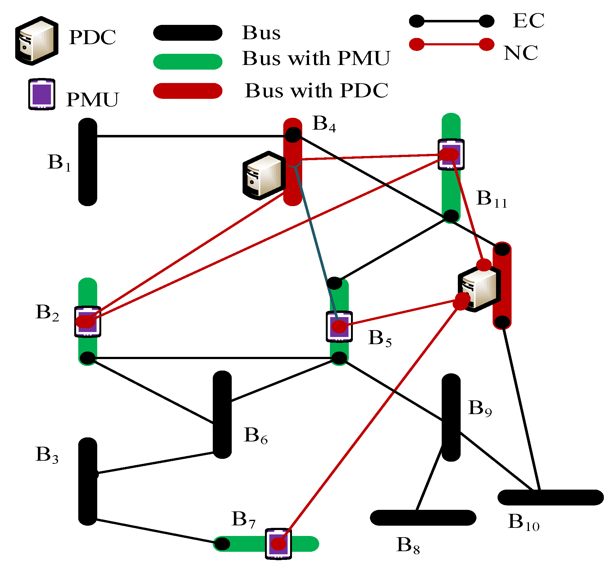
SCNs can be modelled using a graph, where PMU and PDC are represented as the nodes and the communication link between them is represented by an edge in the graph. Let us consider the SCN as shown in Figure 1, where 12 electrical buses are considered. The SCN comprises four PMUs and two PDCs. The buses equipped with a PMU are shown in green, and the buses equipped with a PDC are shown in red. The remaining buses that are neither equipped with a PMU nor a PDC are shown in black. The electrical buses are electrically connected using Electrical Connections (EC), whereas PMUs and PDCs are communicated using Network Connections (NCs).
From the communication network perspective, the PMU, PDC, and their interconnections using NC can be used for analysing SCNs based on a graph-theoretical approach. Let us consider the SCN as a graph G, which is denoted as , where and denote nodes and edges in the graph G. If the SCN has PMUs and PDCs, then the total number of nodes corresponding to PMUs and PDCs in the graph will be . Apart from PMUs and PDCs, there will be many intermediate nodes in the SCNs. If represents the set of intermediate nodes, such that , then the total number of nodes in the network would be . Hence, ; there exists an edge connecting nodes and , such that . We denote the existence of a path between two nodes and as which is defined as an unbroken connection through which one can traverse from node to node . Moreover, path may consist of one or more edges. Thus, a path is a set of all nodes connected by edges joining the source and destination. In a network with more than one path, the different paths will be represented as a set of nodes connected through edges. Path ‘l’ between any source and destination can be represented by , where . Further, the number of paths is given by cardinality i.e., . It should be noted that the graph is assumed undirected to support bidirectional synchrophasor data flow.
For an SCN, it is not necessary to locate the PMUs on all grid buses. The entire system can be observable with a few PMUs located at their optimal locations. However, for the time being, let us assume a simplified diagram where the PMUs, PDCs, and the interconnection between them are as shown in Figure 1.
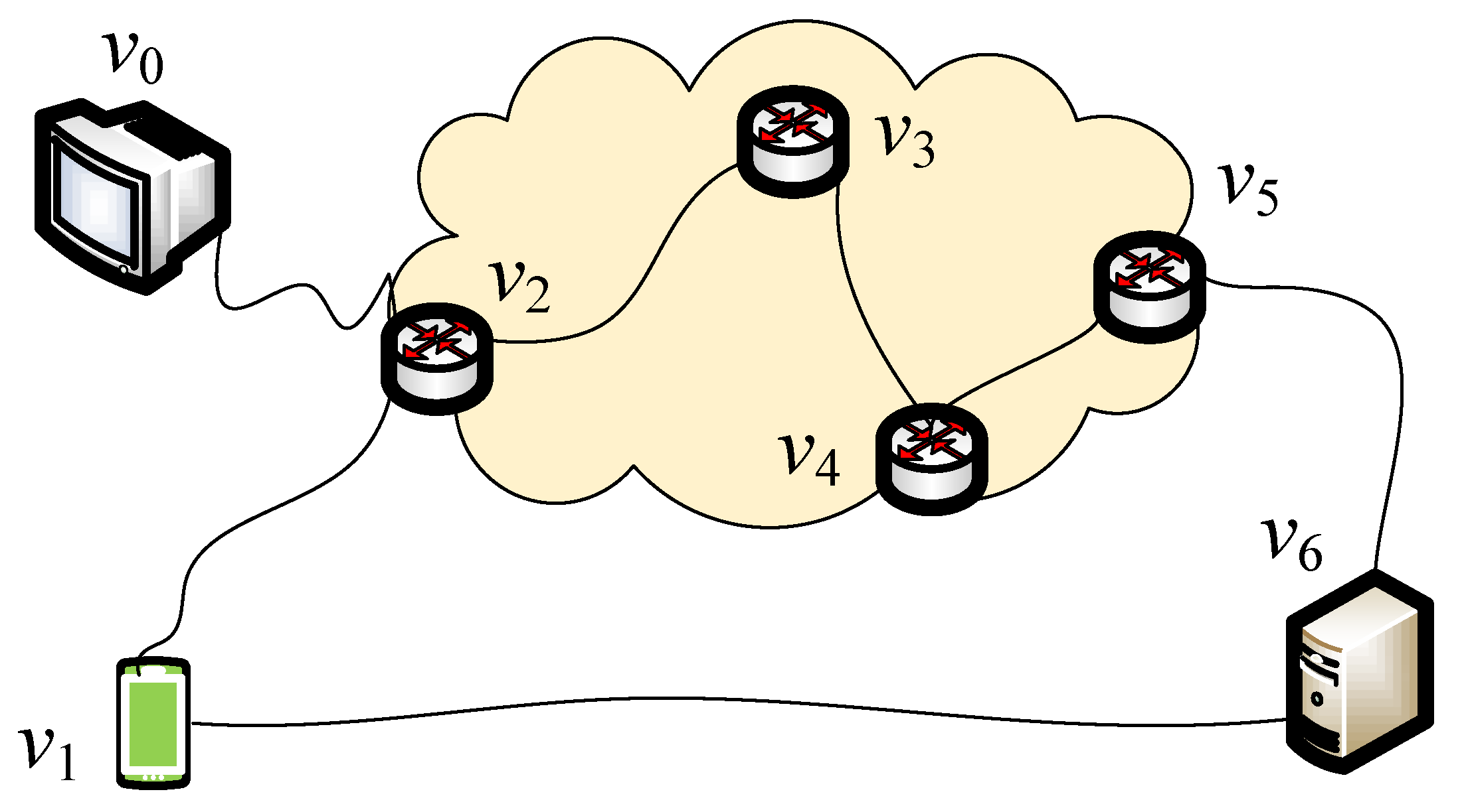
As shown in Figure 1, the PMU and PDC are connected with a single edge that may have many intermediate nodes and edges. For the illustration, the network shown in Figure 2 was constructed from Figure 1 in such a way that a pair of PMU and PDC is connected through many intermediate nodes and edges. In this, node and represent the PMU and the PDC, whereas nodes , and represent intermediate nodes on the IP network. Furthermore, node indicates another device that generates background traffic along with the PMU traffic. It is worth noting that .
3.2. Analysis Metrics
Consider that the synchrophasor data generated at each PMU are ; then, we can define the Packet Delivery Ratio (PDR) as follows.
Packet Delivery Ratio (PDR): For an SCN, if and represent the source and destination nodes, then PDR at node corresponding to node can be defined as:
where is the number of packets received by B at time t, is the number of packets sent by A at time t, is the time at which the first packet is sent from A, is the time at which the last packet is sent from A, is the time at which the first packet is received by B, and is the time at which the last packet is received by B.
3.3. Operation Cycle of SCN
Under a dynamically varying environment, one or more edges can fail partially or fully. For a resilient system, there should be immediate substitution in the service. The requirement of immediate substitution can be achieved by recovering the failed or partially failed edges. Thus, the overall operation of the SCNs can be analysed in the following three states: normal state, partially failed state, and failed state.
3.3.1. Normal State
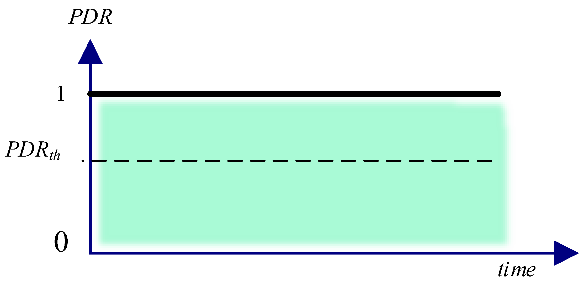
During the normal operation of the SCN, all edges in the network perform normally. Thus, all the PMUs successfully communicate the synchrophasor data to the corresponding PDC. Consequently, the PDR at the PDC corresponding to the PMU remains equal to 1. As an example, using Equation (1), for the PDR at node corresponding to node , we have, and thus .
3.3.2. Partially Failed State
In a partially failed state, the SCN fails partially. Thus, the PDR of the corresponding PMUs is affected. Therefore, for the PMUs with partially failed SCNs, the PDR is always less than 1. As an example, for the PDR at node B corresponding to partially failed node A, we have and thus .
3.3.3. Failed State
In the failed state, the PMU cannot communicate its data to the PDC. Thus, the corresponding to the failed PMUs becomes zero. For example, the at node B corresponding to a failed node A becomes , since .
3.4. State Representation Using Markov Chain
The different states during the operation of the SCN can be modelled using Markov models, as shown in Figure 3.
With respect to the Markov representation of SCN states, let us consider the probabilities of being in the normal, partially failed, and failed states be denoted as , , and respectively. The state transition probabilities are , , , , and for normal to failed, normal to partially failed, partially failed to normal, partially failed to failed, failed to normal, and failed to partially failed states, respectively. As the current state decides the next state and the next state does not depend upon the initial state, the system model satisfies the Markov properties. The resiliency of the synchrophasor communication network can also be described using the Markov chain.
4. Graph Theoretic Resiliency Framework
4.1. Preliminaries of the Resiliency Estimation Framework
The can be calculated at the PDC corresponding to each PMU. Based on the , the overall performance of the SCN can be evaluated. This is because for the normal state, PDR is less than one for a partially failed state, and PDR = 0 for the fully failed state. Thus, we considered the as a Figure of Merit (FoM) for resiliency estimation. Moreover, the average value was considered for the overall system performance, as more than one PMU communicates synchrophasor data to a particular PDC. Thus, the average PDR at the PDC due to the corresponding PMUs can be determined as follows. If there are n PMUs connected to PDC (say, ), then the average at is:
A resiliency curve using the average PDR as a figure of merit is shown in Figure 4 for different instances of time.
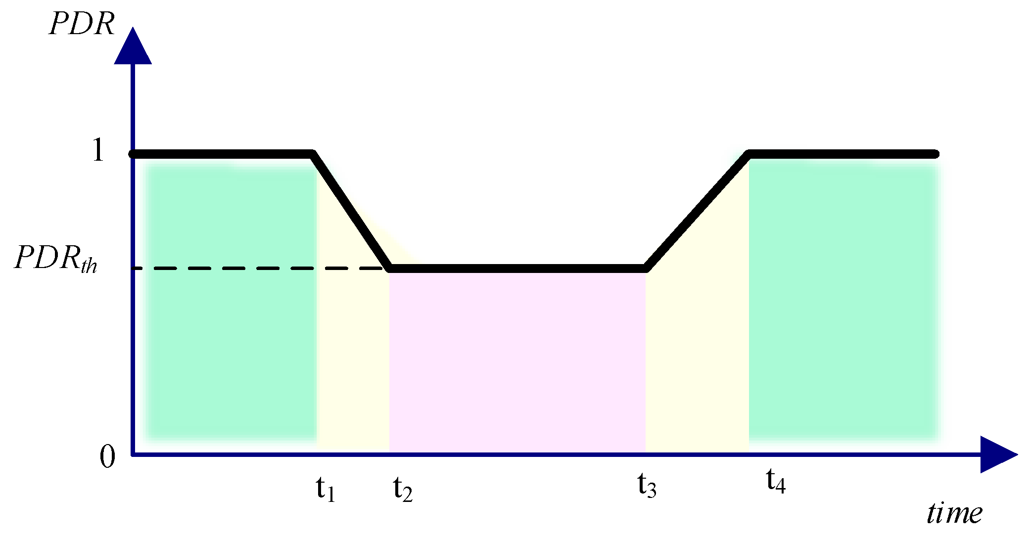
As shown in Figure 4, the SCN is said to be in a normal state when all of its components work normally, resulting in an average PDR of 1. This can be observed up to time . Due to some external/internal factors, some components may fail, which will decrease the average , as shown beyond time . An SCN can tolerate a certain level of reduction in , but in order to perform satisfactorily, it must maintain a minimum value of , which is referred to as the threshold value denoted as . Even during the interval the remains equal to or greater than the threshold value and, thus, the system performs satisfactorily. However, if the PDR becomes less than the threshold value, then the system disrupts and it enters the out-of-service state, i.e., the failed state. This is represented by the decaying exponential (in red colour) beyond time in Figure 4. When the failed components of the system come back to the normal state, then the average PDR will improve, as depicted during . For time , all components recover to their original working state; thus, PDR again reaches the unity value.
The overall operation of the SCN can be studied through the following phases: (1) degradation phase, (2) threshold-operated phase, and (3) recovery phase.
- (1)
- Degradation phase: The phase during which the components of the SCN start failing partially, resulting in the degradation of the . However, the SCN is considered to still be operational, since . The degradation rate () can be defined aswhere and are the received at times and respectively. Thus, if a node degrades at a rate of 0.075 s−1, then it takes 13.34 s to degrade the from 1 to 0.
- (2)
- Threshold-operated phase: This is the state corresponding to the PDR value being close to the threshold value . During this phase, the SCN operates with minimum performance, since some packets may be lost.
- (3)
- Recovery phase: When a partially failed component recovers from the partially failed state to the normal state, or even when a failed component is substituted by normal components, the value increases such that and . The recovery rate can be determined during the recovery phase to using Equation (4), such that .where and are the received at times and , respectively. Thus, if a node recovers at a rate of 0.075 s−1, then it takes 13.34 s to restore the from 0 to 1.
The following vital observation can be noted:
A resilient SCN must follow the resiliency curve shown in Figure 4. However, a highly resilient SCN should preferably have a shorter recovery phase (i.e., min) and a longer degradation phase (i.e., max). It is worth noting that a higher slope for the recovery phase and lower slope for the degradation phase are desirable.
4.2. Resiliency Estimation Framework
Let us consider the network model using the graph approach as described earlier. Now, we consider the representation of the network by an undirected graph, as shown in Figure 2. We assume that there are two paths between the PMU and PDC such that the paths are not distinct, as a node is observed to be common in two paths. To be noted, except for the source and destination nodes, the other nodes between the PMUs and PDCs are not common. Thus, the paths between the PMU and PDC are distinct if the source and destination nodes are ignored.
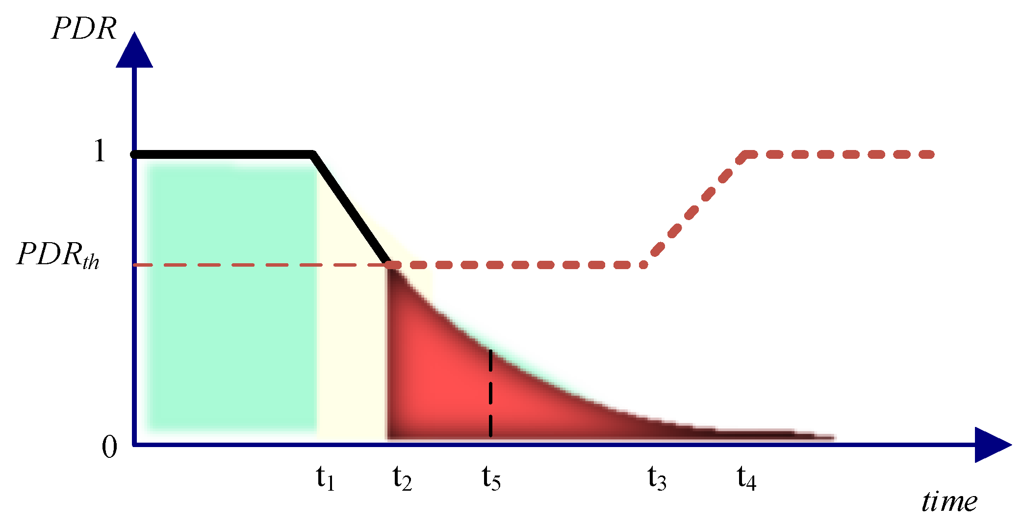
At the beginning, all the nodes in are in their normal states. Furthermore, all links connecting nodes and , such that , are operational. Consequently, the PMU and PDC will be able to exchange the data as the network is operational. Now, consider at time , link partially fails. The failure of this node results in the necessity to reroute the data through another possible path. There will be degradation in the beyond time , and this degradation depends upon the route recovery time (RRT). As node is a shared node having more background traffic than the previous path, the is always less than 1 but greater than threshold value of this path. The can be improved such that becomes close to 1 if, and only if, the failed link is restored to its normal state. This can be seen beyond time in Figure 4.
If the background traffic over link is assumed to be large enough, then the PDR degrades in such a way that PDR becomes less than the threshold value. This results in the disruption of service. The main cause of the disrupted service is the failed state of the link with no backup path, such as through .
Initially, we considered all nodes to be operational. Thus, they participated in the data exchange, resulting in . For simplicity, all nodes and links are assumed to be of equal capacity. Link works as a shared link between the and source–destination pairs. Thus, for equal sharing, half of the link capacity will be used for each of the source–destination pairs, whereas the remaining half will be considered as the background traffic. Thus, for each source–sink pair, there exist two paths: and . Here, the dominant path for the source–destination pair becomes . We assume that the dominant path carries 80% of the data and the other paths carry 20%. It is worth mentioning that the choice of data carried by the dominant path is optional and subject to the researcher’s choice. The exact path between the PMU and PDC for the routing of the data can be estimated by any of the suitable network layer-routing techniques, which is not part of this work. In fact, the routing protocol will be used for the simulation of the network using ns-3. which will be discussed in the later section of proposed work.
Next, the network’s resiliency will be estimated under four cases: normal state, partially failed state, restoration state, and fully failed state.
4.2.1. Case-I: Normal State
In the normal state, the SCN is modelled in a way that all nodes, edges, and, thus, paths are operating under their normal state. In this case, the dominant path is considered to carry 80% of the data for , whereas the redundant shared path is modelled to carry 20% of the PDR data, as the dominant path carries more PDR data. Thus, the overall at destination , corresponding to source , is . The at , corresponding to for the dominant path, is
where , such that , as the nodes are under their normal condition, i.e., no data loss and the dominant path carries 80% of the total traffic generated by the source. Thus,
This implies that
Similarly, for path carrying 20% of the data, . This implies that
Therefore, from Equations (7) and (8),
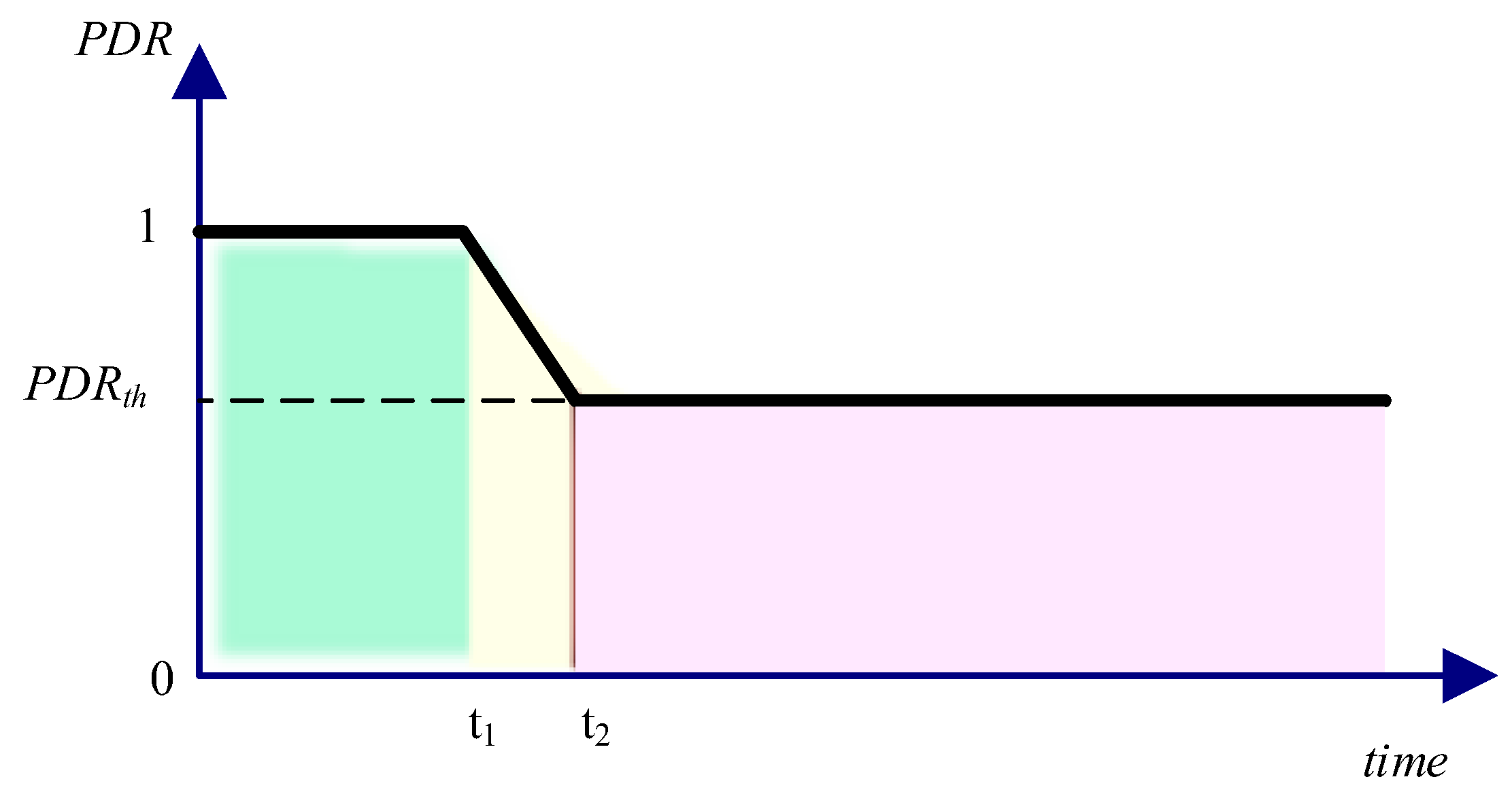
The corresponding resiliency curve corresponding to Case-I is shown in Figure 5.
4.2.2. Case-II: Partially Failed State
It is likely that some of the nodes in the network may not operate normally. As few nodes are subjected to partial failure, the partially failed state is inevitable, which is considered in this section. In this case, we consider that the direct link fails at time . The failure of this node decreases the PDR, as can be deduced from Equation (11).
In this case, due to the partially failed state of a node in dominant path . Thus, all of the traffic generated at node is re-routed to the alternative path if available, such as . Hence, the at the destination node corresponding to path becomes . However, there will be some time for the re-routing of the traffic over path . During this time, the PDR will continue to decrease. Once the new optimum path is detected, then the PDR either increases or maintains the present level. This is shown in the resiliency curve in Figure 6 for the time period to . Moreover, as edge is shared, the corresponding to this path can never reach 1. Hence, the following inequality holds:
Particularly if , the overall at destination corresponding to source can be produced by,
Therefore, the following inequality holds:
The corresponding resiliency curve is shown in Figure 6. As , the network is considered to be functional in this case. It is worth noting that, for a network Ɲ, if . Thus, for non-zero , there must exist an alternative path between source–destination pairs.
4.2.3. Case-III: Restoration State
In this case, we consider that the failed edge in the previous case starts to repair itself either by substitution or recovery at time . Upon recovery, the failed edge restores the path , which increases the , as can be deduced from Equation (16).
In this case, the corresponding to the dominant path increases such that . The restoration will be achieved over a certain time span, such as to such that, at , .
Further, with the restoration of dominant path , the traffic from path will be off-loaded and diverted to dominant path . This is because the dominant path is considered to be dedicated, whereas the path is shared. Hence, the at the destination node corresponding to path becomes , such that, at , . There will be some time for the re-routing of the traffic over path . During this time span, the will continue increasing.
The overall at destination corresponding to source can be given by
Thus, at , . Therefore, the following inequality holds:
The corresponding resiliency curve is shown in Figure 7, where the restoration phase is shown through the interval to . Nevertheless, as , the network is considered to be functional in this case.
4.2.4. Case-IV: Failed State
In this state, we consider that node fails permanently at time . The failure of this node decreases the PDR, as can be deduced from Equation (20).
In this case, due to the fully failed state of a node in the dominant path . Thus, all of the traffic generated at node must be re-routed to path . If there exists no such path, i.e., for an SCN Ɲ with , then it can be clearly seen that the decreases, such that at Moreover, even though there exists such a path with , the systems loses its functionality. For an instance, decreases beyond and at . This is shown in Figure 8 for time span to .
5. Simulation Results and Discussion
Based on the resiliency estimation framework discussed in the last section, we propose a simulation framework to estimate the resiliency of the SCN using ns-3.
5.1. SCN Design and Implementation
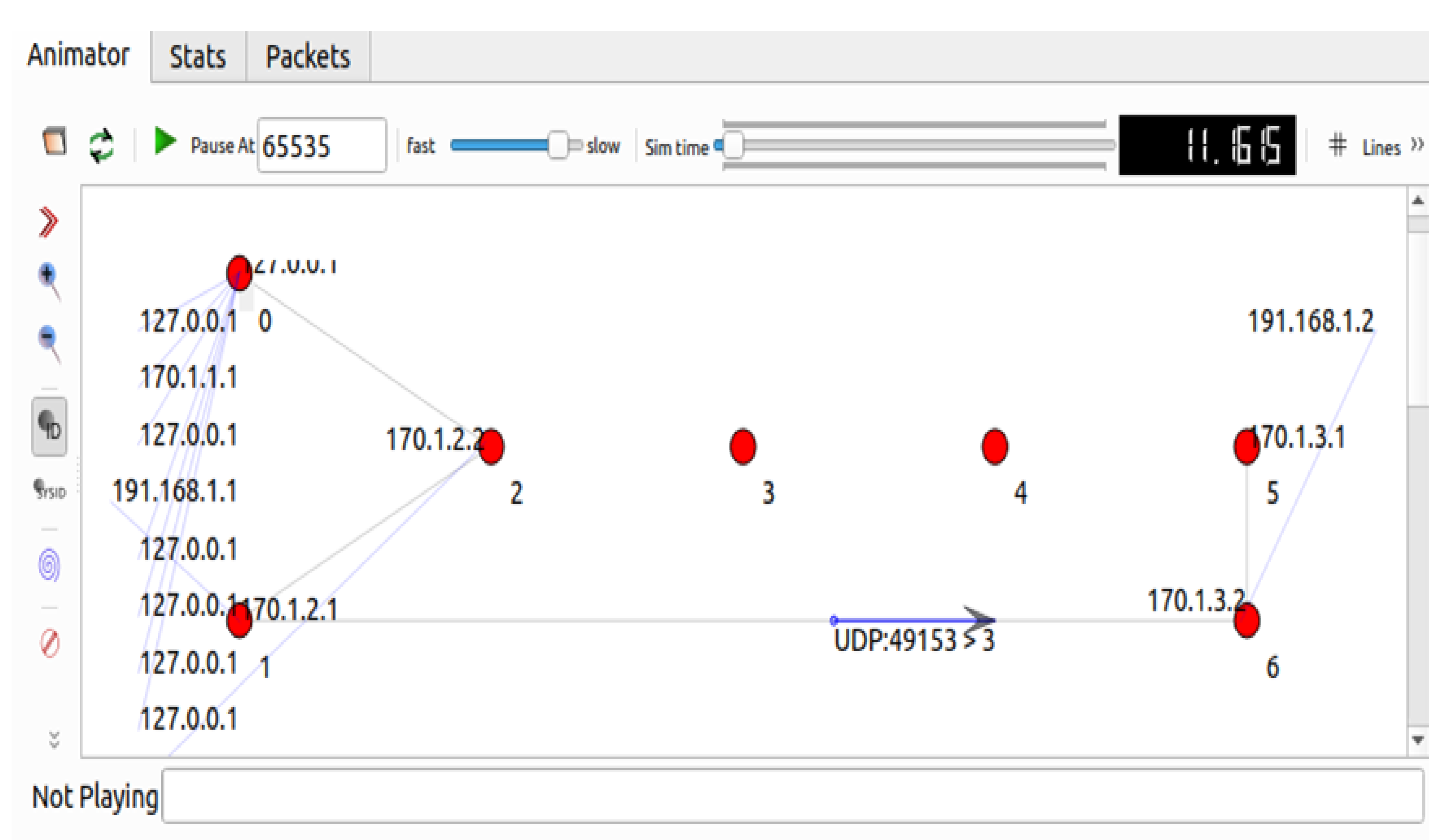
We will consider the network topology shown in Figure 2. The parameters of the SCN are selected in conjunction with the synchrophasor application described in [30]. The deployment of the network involves the configuration of five networks described as follows. Network Ɲ1 connects the PMU and PDC through a dedicated point-to-point channel with network address 191.168.1.0. The Internet is modelled using network Ɲ2, where nodes v2, v3, v4, and v5 are intermediate routers that can be configured to mimic the behaviour of the Internet, such as background traffic, routing data, etc. To provide alternative routes to the PMU and PDC, we consider two more networks, Ɲ3 and Ɲ4. Network Ɲ3 connects the PMU to the Internet using node , whereas the PDC is connected to the Internet using network Ɲ4 with the help of node The network addresses of networks Ɲ3 and Ɲ4 are 170.1.2.0 and 170.1.3.0, respectively. Furthermore, to model the background traffic over the Internet, network Ɲ5 is constructed, which connects a node generating background traffic (corresponding to the PDR data flow) to the Internet Ɲ2. The network address for network Ɲ5 is 170.1.1.0. It should be noted that all networks are designed in the class-B hierarchy. The design and implementation of the SCN in ns-3 are shown in Figure 9.
5.2. Network Parameters and Configurations
As discussed, the simulation scenario under consideration includes a total of five networks, Ɲ1, Ɲ2, Ɲ3, Ɲ4, and Ɲ5. These networks are implemented in ns-3 and are shown in Figure 9. Some of the key parameters used for the configuration of these networks in ns-3 are comprehensively summarized in Table 1.
Each node in the network is configured with the dynamic global routing protocol to populate the routing data for routing. The OSPF protocol is used as a dynamic global routing protocol that works on link-state algorithms to discover networks, find optimum paths, and maintain the routing information. In ns-3, the dynamic global routing protocol in a node is configured using the following command: Ipv4GlobalRoutingHelper::PopulateRoutingTables(), which enables routing capability in all nodes during simulation. This function calls other ns-3 functions, BuildGlobalRoutingDatabase () and InitializeRoutes (), to build a routing database and initialize routing tables, respectively. Nodes v1 and v6 are used as the source and destination, respectively. The PMU is configured with the CBR applications supported by the UDP transport protocol to generate the application at a data rate of 300 Kbps. In particular, an on–off application helper is used to create an application in ns-3. The desired data rate in ns-3 can be set using Equation (21). To achieve a PMU data rate equal to 300 Kbps, the 25 packets/s that result in a packet transmission time of 1/25 s are considered, with each packet being equal to 1.5 KB. In ns-3, such applications with the desired data rate are configured using OnOffHelper.
5.3. Simulation Results
The key simulation parameters for the SCN in ns-3 are summarized in Table 2.
The network is designed and configured, and events are scheduled per the requirements referring to Table 1 and Table 2. The network is simulated under three cases for effectively analysing the resiliency of the synchrophasor communication network, which will be discussed subsequently. Nevertheless, the network animation remains the same for all cases.
5.3.1. Case I: Complete Link Failure with No Backup Path
In this case, we configure the SCN Ɲ in such a way that there is no backup path. This can be configured by disabling network Ɲ4. Furthermore, network Ɲ1 is disabled for 50 s to 110 s. The SCN is simulated for 110 s.
5.3.2. Case II: Complete Link Failure with a Partially Failed Backup Path
In this case, we configure the SCN Ɲ in such a way that a backup path exists. The backup path is considered through the Internet, which is modelled using network Ɲ2. Node v1 is connected to the Internet through network Ɲ3. Node v6 is connected to the Internet through network Ɲ4. Thus, the backup path comprises networks Ɲ2, Ɲ3, and Ɲ4. To configure the backup path in the partially failed state, we configure the Internet with 75% background traffic. Furthermore, network Ɲ1 is disabled for 150 s to 210 s. The SCN is simulated from 110 s to 210 s.
5.3.3. Case III: Link Failure with a High-Capacity Backup Path
Here, we configure the SCN Ɲ in such a way that there exists a backup path that has sufficient capacity to support the data rate generated at source node v1. Like the last case study, the backup path is considered to be through the Internet, which is modelled using network Ɲ2. Node v1 is connected to the Internet through network Ɲ3. Node v6 is connected to the Internet through network Ɲ4. Thus, the backup path comprises networks Ɲ2, Ɲ3, and Ɲ4. To configure a high-capacity backup path, networks Ɲ2, Ɲ3, and Ɲ4 are configured with data rates , , and , respectively, such that , where is the data rate at v1. In particular, the bandwidth of the channel belonging to networks Ɲ1, Ɲ2, Ɲ3, and Ɲ5 is considered to be 2 Mbps. The bandwidth of network Ɲ4 is also considered to be 2 Mbps. However, its effective available bandwidth is variable, subject to the applied background traffic. To elaborate, the effective available bandwidth for the PMU data rate becomes only 1Mbps when network Ɲ4 is subjected to 50% background traffic. In a nutshell, PointToPointHelper and CsmaHelper syntax in ns-3 are used to configure different attributes related to the dedicated and shared CSMA channels, respectively. After configuring all network parameters, network Ɲ1 is disabled for 240 s to 280 s. Moreover, the SCN is simulated for 300 s.
5.4. Discussion of ns-3 Simulation Results
The simulation results are summarized in Table 3.
When the network is simulated for 50 s, since network Ɲ1 is operational, data are communicated over this network from the PMU with an IP address of 191.168.1.1 to the PDC with an IP address of 170.1.3.2. The PMU communicates 1224 packets to the PDC with a packet loss ratio of 0%. Thus, all packets are received at the PDC, which results in a PDR value equal to 1. This can also be validated using Table 3.
When the network is simulated for 110 sec, since network Ɲ1 is operational only up to 50 s, data are communicated over this network from the PMU at interface 191.168.1.1 to the PDC at interface 170.1.3.2 up to 50 s only. Further, the PDC receives all 1224 packets sent from the PMU through interface 191.168.1.1, as the packet loss ratio is 0% at the 170.1.3.2 interface of the PDC corresponding to this flow.
For the simulation beyond 50 s and up to 110 s, as network Ɲ1 fails, no data can be communicated using this network. In response to the failure of network Ɲ1, the PMU reroutes data through the alternative route at interface 170.1.2.1, which is through network Ɲ3 over the Internet Ɲ2. Nevertheless, network Ɲ4 is disabled to ensure the absence of a backup path between the PMU and PDC. Therefore, PDC does not receive data corresponding to this flow as the packet loss ratio is 100% at the 170.1.3.2 interface of the PDC. Consequently, the drops to 0 for the simulation from 50 s up to 110 s. This can also be corroborated by Table 3.
When the network is simulated for 210 s, then network Ɲ1 fails again (first failure in case study-I) at 150 s and remains in the failed state up to 210 s. Therefore, no data can be communicated by the PMU over this network from the PMU at interface 191.168.1.1 to the PDC at interface 170.1.3.2 from 150 s to 210 s. This can be verified, as the last packet transmitted corresponding to this flow is at 149.96 s. Moreover, network Ɲ1 is operational for up to 150 s. Thus, the PDC receives all 2224 packets transmitted by the PMU. Thus, all packets are received at the PDC, which results in a PDR value equal to 1 for this flow.
For simulation beyond 150 s and up to 210 s, as network Ɲ1 remains failed, no further data can be communicated using this network. In response to the failure of network Ɲ1, the PMU reroutes data through an alternative route at interface 170.1.2.1, which is through network Ɲ3 over the Internet Ɲ2. Nevertheless, network Ɲ4 is now available, but configured with 75% background traffic (with a data rate of 10 Kbps). This ensures the existence of a backup path between the PMU and PDC. Therefore, the PDC receives 1995 packets out of 3000 transmitted packets by the PMU at interface 170.1.2.1, resulting in a packet loss ratio of 30.7051%. Consequently, the performance of the network in terms of the PDR is better as compared with case study-I. Specifically, the average PDR corresponding to both flows is equal, corroborated by Table 3.
When the network is simulated for 280 s, network Ɲ1 is configured to fail again (first failure in case study-I and second failure in case study-II) at 240 s and remains failed up to 280 s. Therefore, no data can be communicated by the PMU over this network from the PMU at interface 191.168.1.1 to the PDC at interface 170.1.3.2 from 240 s to 280 s. This can be verified as the last packet transmitted at 239.96 s corresponds to this flow.
For this simulation period, in response to the failure of network Ɲ1, the PMU reroutes data through an alternative route at interface 170.1.2.1, which is through network Ɲ3 over the Internet Ɲ2. Nevertheless, network Ɲ4 is now available and configured with only 25% background traffic (with a data rate of 30 Kbps). This ensures a backup path with sufficiently high bandwidth between the PMU and PDC. Therefore, the PDC receives all 4000 packets transmitted by the PMU at interface 170.1.2.1, resulting in a packet loss ratio of 0%. Consequently, the performance of the network in terms of is superior to that in earlier case studies. Specifically, the average PDR corresponding to both flows is equal, which can be corroborated by Table 3.
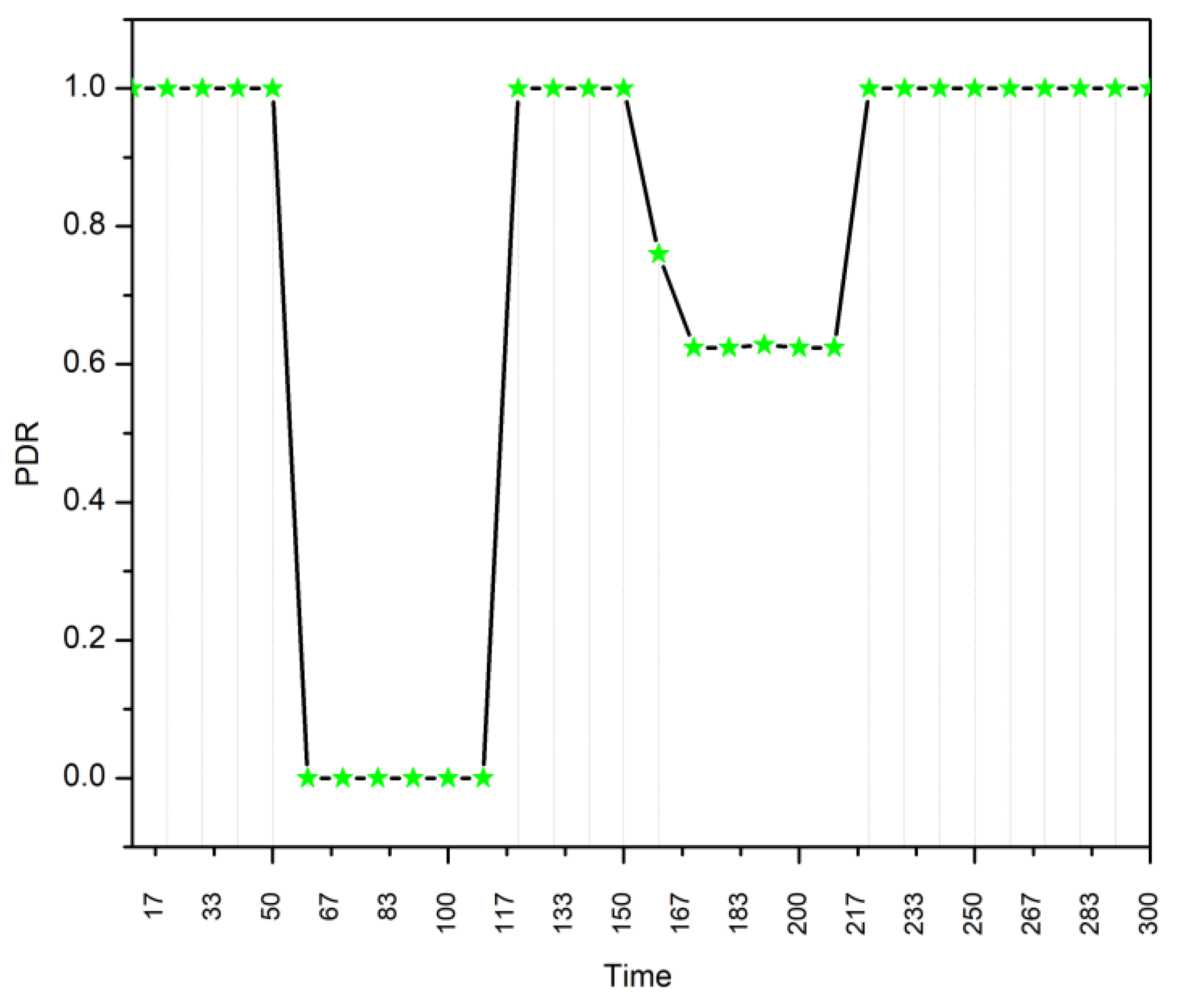
A graph of PDR as a function of the simulation time corresponding to all case studies is plotted in Figure 10. From the figure, it can be seen that the first failure event of network Ɲ1 occurs at 50 s. Before the failure of the network, the PDR remains equal to 1. As there is no backup path under this case study, PDR drops to 0 in response to the failure event. Moreover, during the 50 s to 110 s simulation time, PDR remains at 0. Thus, the SCN loses its functionality.
Furthermore, the degradation rate using Equation (3) can be estimated to be . From Figure 10, s, s, , and . The performance graph for case study-II shows the period of 110 s to 210 s. Network Ɲ1 restores at 110 s, which improves the to 1 compared with the failure event of case study-I, where the PDR is 0. Furthermore, the recovery rate using the equation can be estimated to be . From Figure 10, , , , and . Here, network Ɲ1 fails again at 150 s; thus, the PDR degrades. However, the PDR does not become 0, i.e., . Moreover, the degradation rate using Equation (3) can be estimated to be . From Figure 10, , , , and . Further, the recovery rate using Equation (4) can be estimated to be . From Figure 10, , , , and .
Hence, the performance of the SCN is better in the event of a failure than in the earlier case study, where there is no alternative route. Moreover, the recovery rate is better when network Ɲ1 restores at 110 s as compared with that at 210 s. The performance graph for case study-III shows the period from 210 s to 300 s. Network Ɲ1 restores at 210 s, which improves the PDR to 1 compared with the failure events of case study-II and, of course, case study-I. Here, network Ɲ1 fails again at 240 s. However, the PDR remains at 1, as a backup path with sufficiently large bandwidth exists. Hence, it is conclusive that the performance of the SCN is superior to that in the earlier case studies in the event of failure.
5.5. Some Future Research Directions
SCNs are vital to the success of SGs as they provide real-time monitoring capabilities to the marvellous power system. In this paper, an approach was presented in the resiliency evaluation paradigm. Some of the future research directions to further augment the resiliency paradigm are enumerated below:
- The dynamic characteristics of all the nodes in terms of failure, repair, etc. can be studied for resiliency analysis of the SCN;
- The effect of variable bandwidth on all channels can be studied to observe the performance of the SCN in terms of resiliency parameters;
- A more complex SCN can be modelled and the presented work can be extended on such a complex SCN for resiliency analysis;
- A more peculiar SCN model can be developed with the objective of designing a testbed for SG design, implementation, and performance evaluation;
- Last, but not least, more comprehensive definitions and resiliency metrics can be proposed in future work.
6. Conclusions and Future Work
The synchrophasor communication network of a smart grid caters to the basic needs to meet the goals of the smart grid. The SCN is subjected to several challenges leading to operational hindrances. To overcome such issues, resiliency estimation of an SCN of an SG was considered in this paper. To evaluate the resiliency estimation, a simplified graph-theoretic approach was presented to model the SCN analytically. An SCN was designed, implemented, and simulated using a discrete event-based network simulator, ns-3. The resiliency estimation was conducted with the packet delivery ratio as a figure of merit. Nevertheless, the proposed graph-theoretic-based resiliency framework can be regarded as the first such attempt that can be extended to generic communication networks. The inclusion of a case study is considered future work. With respect to case study-I, the SCN was observed to lose its functionality, such that and . Contrary to case study-I, the SCN remained in a functional state in case study-II, with and . If the bandwidth available is sufficiently large compared with the background traffic and synchrophasor data rate, then an SCN with at least one backup path remains fully functional (normal state), as observed in case study-III.
Author Contributions
Conceptualization, A.V.J.; methodology, A.V.J.; software, A.V.J.; validation, B.A.; formal analysis, A.V.J. and B.A.; investigation, N.B. and P.T.; resources, B.A. and N.B.; data curation, A.V.J.; writing—original draft preparation, A.V.J.; supervision, N.B. and B.A.; project administration, N.B. and P.T.; funding acquisition, P.T.; writing—review and editing: A.V.J., B.A., P.T. and N.B. All authors have read and agreed to the published version of the manuscript.
Funding
This work was supported in part by the Framework Agreement between the University of Pitesti (Romania) and King Mongkut’s University of Technology North Bangkok (Thailand), in part by an International Research Partnership “Electrical Engineering—Thai French Research Center (EE-TFRC)” under the project framework of the Lorraine Université d’Excellence (LUE) in cooperation between Université de Lorraine and King Mongkut’s University of Technology North Bangkok, and in part by the National Research Council of Thailand (NRCT) under Senior Research Scholar Program under Grant No. N42A640328.
Institutional Review Board Statement
Not applicable.
Informed Consent Statement
Not applicable.
Data Availability Statement
Not applicable.
Conflicts of Interest
The authors declare no conflict of interest.
References
- Fotis, G.; Dikeakos, C.; Zafeiropoulos, E.; Pappas, S.; Vita, V. Scalability and replicability for smart grid innovation projects and the improvement of renewable energy sources exploitation: The flexitranstore case. Energies 2022, 15, 4519. [Google Scholar] [CrossRef]
- Rahim, S.; Siano, P. A survey and comparison of leading-edge uncertainty handling methods for power grid mod-ernization. Expert Syst. Appl. 2022, 204, 117590. [Google Scholar] [CrossRef]
- Aguero, J.R.; Novosel, D.; Bernabeu, E.; Chiu, B.; Liu, J.; Rabl, V.; Pierpoint, T.; Houseman, D.; Enayati, B.; Kolluri, S. Managing the new grid: Delivering sustainable electrical energy. IEEE Power Energy Mag. 2019, 17, 75–84. [Google Scholar] [CrossRef]
- Dileep, G. A survey on smart grid technologies and applications. Renew. Energy 2019, 146, 2589–2625. [Google Scholar]
- Masera, M.; Bompard, E.F.; Profumo, F.; Hadjsaid, N. Smart (Electricity) Grids for Smart Cities: Assessing Roles and Societal Impacts. Proc. IEEE 2018, 106, 613–625. [Google Scholar] [CrossRef]
- Haes Alhelou, H.; Hamedani-Golshan, M.E.; Njenda, T.C.; Siano, P. A Survey on Power System Blackout and Cascading Events: Research Motivations and Challenges. Energies 2019, 12, 682. [Google Scholar] [CrossRef] [Green Version]
- Leibovich, P.; Issouribehere, F.; Barbero, J. IoT Platforms for WAMS Systems: A complete Synchrophasor Measurement System in the Cloud. In Proceedings of the 2022 IEEE Power & Energy Society General Meeting (PESGM), Denver, CO, USA, 17–21 July 2022; pp. 1–5. [Google Scholar] [CrossRef]
- Jha, A.V.; Appasani, B.; Ghazali, A.N.; Pattanayak, P.; Gurjar, D.S.; Kabalci, E.; Mohanta, D.K. Smart grid cyber-physical systems: Communication technologies, standards and challenges. Wirel. Netw. 2021, 27, 2595–2613. [Google Scholar] [CrossRef]
- Yan, Y.; Qian, Y.; Sharif, H.; Tipper, D. A Survey on Smart Grid Communication Infrastructures: Motivations, Requirements and Challenges. IEEE Commun. Surv. Tutorials 2012, 15, 5–20. [Google Scholar] [CrossRef] [Green Version]
- Sufyan, M.A.A.; Zuhaib, M.; Rihan, M. Applications of Synchrophasors Technology in Smart Grid. In Advances in Clean Energy Technologies; Baredar, P.V., Tangellapalli, S., Solanki, C.S., Eds.; Springer: Singapore, 2021; pp. 745–758. [Google Scholar] [CrossRef]
- Khan, R.H.; Khan, J.Y. Wide area PMU communication over a WiMAX network in the smart grid. In Proceedings of the 2012 IEEE Third International Conference on Smart Grid Communications (SmartGridComm), Tainan, Taiwan, 5–8 November 2012; pp. 187–192. [Google Scholar]
- Kwasinski, A.; Weaver, W.W.; Chapman, P.L.; Krein, P.T. Telecommunications power plant damage assessment for hurricane katrina–site survey and follow-up results. IEEE Syst. J. 2009, 3, 277–287. [Google Scholar] [CrossRef]
- Chenine, M.; Nordstrom, L. Investigation of communication delays and data incompleteness in multi-PMU wide area monitoring and control systems. In Proceedings of the 2009 International Conference on Electric Power and Energy Conversion Systems (EPECS), Sharjah, United Arab Emirates, 10–12 November 2009; pp. 1–6. [Google Scholar]
- Danielson, C.F.M.; Vanfretti, L.; Almas, M.S.; Choompoobutrgool, Y.; Gjerde, J.O. Analysis of communication network challenges for synchrophasor-based wide-area applications. In Proceedings of the 2013 IREP Symposium Bulk Power System Dynamics and Control-IX Optimization, Security and Control of the Emerging Power Grid, Rethymnon, Greece, 25–30 August 2013; pp. 1–13. [Google Scholar]
- Hosseini, S.; Barker, K.; Ramirez-Marquez, J.E. A review of definitions and measures of system resilience. Reliab. Eng. Syst. Saf. 2016, 145, 47–61. [Google Scholar] [CrossRef]
- Jha, A.V.; Appasani, B.; Ghazali, A.N. Performance Evaluation of Routing Protocols in Synchrophasor Communication Networks. In Proceedings of the 2019 International Conference on Information Technology (ICIT), Bhubaneswar, India, 19–21 December 2019; pp. 132–136. [Google Scholar] [CrossRef]
- Katsaros, K.V.; Yang, B.; Chai, W.K.; Pavlou, G. Low latency communication infrastructure for synchrophasor applications in distribution networks. In Proceedings of the 2014 IEEE International Conference on Smart Grid Communications (SmartGridComm), Venice, Italy, 3–6 November 2014; pp. 392–397. [Google Scholar]
- Jha, A.V.; Appasani, B.; Ghazali, A.N.; Bizon, N. A Comprehensive Risk Assessment Framework for Synchrophasor Communication Networks in a Smart Grid Cyber Physical System with a Case Study. Energies 2021, 14, 3428. [Google Scholar] [CrossRef]
- Castello, P.; Muscas, C.; Pegoraro, P.A.; Sulis, S. Adaptive management of synchrophasor latency for an active phasor data concentrator. In Proceedings of the 2017 IEEE International Instrumentation and Measurement Technology Conference (I2MTC), Turin, Italy, 22–25 May 2017; pp. 1–6. [Google Scholar]
- Das, S.; Sidhu, T.S. Application of Compressive Sampling in Synchrophasor Data Communication in WAMS. IEEE Trans. Ind. Informatics 2013, 10, 450–460. [Google Scholar] [CrossRef]
- Zhu, X.; Wen, M.H.F.; Li, V.O.K.; Leung, K.-C. Optimal PMU-Communication link placement for smart grid wide-area measurement systems. IEEE Trans. Smart Grid 2018, 10, 4446–4456. [Google Scholar] [CrossRef]
- Jha, A.V.; Ghazali, A.N.; Appasani, B.; Ravariu, C.; Srinivasulu, A. Reliability analysis of smart grid networks Iincorporating hardware failures and packet loss. Rev. Roum. Sci. Tech. El 2021, 65, 245–252. [Google Scholar]
- Seyedi, Y.; Karimi, H.; Wetté, C.; Sansò, B. A New Approach to Reliability Assessment and Improvement of Synchrophasor Communications in Smart Grids. IEEE Trans. Smart Grid 2020, 11, 4415–4426. [Google Scholar] [CrossRef]
- Appasani, B.; Jha, A.V.; Mishra, S.K.; Ghazali, A.N. Communication infrastructure for situational awareness enhancement in WAMS with optimal PMU placement. Prot. Control Mod. Power Syst. 2021, 6, 1–12. [Google Scholar] [CrossRef]
- Jha, A.V.; Appasani, B.; Ghazali, A.N. A Comprehensive Framework for the Assessment of Synchrophasor Com-munication Networks from the Perspective of Situational Awareness in a Smart Grid Cyber Physical System. Technol. Econ. Smart Grids Sustain. Energy 2022, 7, 1–18. [Google Scholar] [CrossRef]
- Appasani, B.; Jha, A.V.; Swain, K.; Cherukuri, M.; Mohanta, D.K. Resiliency Estimation of Synchrophasor Com-munication Networks in a Wide Area Measurement System. Front. Energy Res. 2022, 10. [Google Scholar] [CrossRef]
- Jha, A.V.; Appasani, B.; Ustun, T.S. Resiliency assessment methodology for synchrophasor communication networks in a smart grid cyber–physical system. Energy Rep. 2022, 8, 1108–1115. [Google Scholar] [CrossRef]
- Jha, A.V.; Appasani, B.; Gupta, D.K.; Ustun, T.S. Analytical Design of Synchrophasor Communication Networks with Resiliency Analysis Framework for Smart Grid. Sustainability 2022, 14, 15450. [Google Scholar] [CrossRef]
- Khan, R.H.; Khan, J. A comprehensive review of the application characteristics and traffic requirements of a smart grid communications network. Comput. Netw. 2013, 57, 825–845. [Google Scholar] [CrossRef]
- IEEE Std C37118-2005; IEEE Standard for Synchrophasor Data Transfer for Power Systems. IEEE Std C371182-2011 Revis; IEEE: Piscataway, NJ, USA, 2011; pp. 1–53.
Figure 1.
Illustration of an SCN for graph-theoretical modelling.

Figure 2.
Simplified model of an SCN for the graph-theoretic approach.

Figure 3.
Morkov representation of different states of SCN operation.

Figure 4.
Resiliency curve.

Figure 5.
Resiliency curve of the SCN model for Case-I.

Figure 6.
Resiliency curve of the SCN model for Case-II.

Figure 7.
Resiliency curve of the SCN model for Case-III.

Figure 8.
Resiliency curve of the SCN model for Case-IV.

Figure 9.
SCN design using ns-3.

Figure 10.
Resiliency curve using the simulation framework of the SCN.


Table 1.
Key ns-3 configuration parameters for the SCN.
| Network | Network Address | Parameters | Remarks | |
|---|---|---|---|---|
| Data Rate (Kbps) | Delay (ms) | |||
| Ɲ1 | 191.168.1.0 | 2000 | 2 | Dedicated network for PMU and PDC |
| Ɲ2 | 191.88.1.0 | 2000 | 2 | Mimics the Internet |
| Ɲ3 | 170.1.2.0 | 2000 | 2 | Backup path |
| Ɲ4 | 170.1.3.0 | Variable | 2 | Backup path |
| Ɲ5 | 170.1.1.0 | 2000 | 2 | Background traffic |
Table 2.
Some of the key simulation parameters for the SCN.
| Simulation Parameters | Value |
|---|---|
| Application | UDP (Packet Size = 50 KB, Data rate = 10 Kbps) |
| Simulation start at (s) | 0.001 |
| Simulation stop at (s) | 300 |
| Application start at (s) | 1 |
| Application stop at (s) | 299 |
| Point-to-point link fails at (s) | 50 |
| Point-to-point link restores at (s) | 110 |
| Point-to-point link fails at (s) | 140 |
| Point-to-point link restores at (s) | 210 |
| Point-to-point link fails at (s) | 240 |
| Point-to-point link restores at (s) | 280 |
Table 3.
NS-3 simulation results for the SCN based on the graph-theoretic approach.
| Observation | Number of Packets Sent | Number of Packets Received at 170.1.3.2 | Total Number of Packets Sent | Total Number of Packets Received | PDR | ||||
|---|---|---|---|---|---|---|---|---|---|
| Start Time (s) | Stop Time (s) | From Source Interface | From Source Interface | ||||||
| 191.168.1.1 | 170.1.2.1 | 191.168.1.1 | 170.1.2.1 | ||||||
| Case study I | 0 | 10 | 224 | 0 | 224 | 0 | 224 | 224 | 1 |
| 10 | 20 | 250 | 0 | 250 | 0 | 250 | 250 | 1 | |
| 20 | 30 | 250 | 0 | 250 | 0 | 250 | 250 | 1 | |
| 30 | 40 | 250 | 0 | 250 | 0 | 250 | 250 | 1 | |
| 40 | 50 | 250 | 0 | 250 | 0 | 250 | 250 | 1 | |
| 50 | 60 | 0 | 250 | 0 | 0 | 250 | 0 | 0 | |
| 60 | 70 | 0 | 250 | 0 | 0 | 250 | 0 | 0 | |
| 70 | 80 | 0 | 250 | 0 | 0 | 250 | 0 | 0 | |
| 80 | 90 | 0 | 250 | 0 | 0 | 250 | 0 | 0 | |
| 90 | 100 | 0 | 250 | 0 | 0 | 250 | 0 | 0 | |
| 100 | 110 | 0 | 250 | 0 | 0 | 250 | 0 | 0 | |
| Case study II | 110 | 120 | 249 | 0 | 249 | 0 | 249 | 249 | 1 |
| 120 | 130 | 251 | 0 | 251 | 0 | 251 | 251 | 1 | |
| 130 | 140 | 250 | 0 | 250 | 0 | 250 | 250 | 1 | |
| 140 | 150 | 250 | 0 | 250 | 0 | 250 | 250 | 1 | |
| 150 | 160 | 0 | 250 | 0 | 190 | 250 | 190 | 0.76 | |
| 160 | 170 | 0 | 250 | 0 | 156 | 250 | 156 | 0.624 | |
| 170 | 180 | 0 | 250 | 0 | 156 | 250 | 156 | 0.624 | |
| 180 | 190 | 0 | 250 | 0 | 157 | 250 | 157 | 0.628 | |
| 190 | 200 | 0 | 250 | 0 | 156 | 250 | 156 | 0.624 | |
| 200 | 210 | 0 | 250 | 0 | 156 | 250 | 156 | 0.624 | |
| Case study III | 210 | 220 | 250 | 0 | 250 | 0 | 250 | 250 | 1 |
| 220 | 230 | 250 | 0 | 250 | 0 | 250 | 250 | 1 | |
| 230 | 240 | 250 | 0 | 250 | 0 | 250 | 250 | 1 | |
| 240 | 250 | 0 | 250 | 0 | 250 | 250 | 250 | 1 | |
| 250 | 260 | 0 | 250 | 0 | 250 | 250 | 250 | 1 | |
| 260 | 270 | 0 | 250 | 0 | 250 | 250 | 250 | 1 | |
| 270 | 280 | 0 | 250 | 0 | 250 | 250 | 250 | 1 | |
| 280 | 290 | 250 | 0 | 250 | 0 | 250 | 250 | 1 | |
| 290 | 300 | 225 | 0 | 225 | 0 | 225 | 225 | 1 | |
Disclaimer/Publisher’s Note: The statements, opinions and data contained in all publications are solely those of the individual author(s) and contributor(s) and not of MDPI and/or the editor(s). MDPI and/or the editor(s) disclaim responsibility for any injury to people or property resulting from any ideas, methods, instructions or products referred to in the content. |
© 2023 by the authors. Licensee MDPI, Basel, Switzerland. This article is an open access article distributed under the terms and conditions of the Creative Commons Attribution (CC BY) license (https://creativecommons.org/licenses/by/4.0/).
Share and Cite
MDPI and ACS Style
Jha, A.V.; Appasani, B.; Bizon, N.; Thounthong, P. A Graph-Theoretic Approach for Modelling and Resiliency Analysis of Synchrophasor Communication Networks. Appl. Syst. Innov. 2023, 6, 7. https://doi.org/10.3390/asi6010007
AMA Style
Jha AV, Appasani B, Bizon N, Thounthong P. A Graph-Theoretic Approach for Modelling and Resiliency Analysis of Synchrophasor Communication Networks. Applied System Innovation. 2023; 6(1):7. https://doi.org/10.3390/asi6010007
Chicago/Turabian StyleJha, Amitkumar V., Bhargav Appasani, Nicu Bizon, and Phatiphat Thounthong. 2023. "A Graph-Theoretic Approach for Modelling and Resiliency Analysis of Synchrophasor Communication Networks" Applied System Innovation 6, no. 1: 7. https://doi.org/10.3390/asi6010007