Forecasting Seasonal Sales with Many Drivers: Shrinkage or Dimensionality Reduction?

Abstract

Retailers depend on accurate forecasts of product sales at the Store × SKU level to efficiently manage their inventory. Consequently, there has been increasing interest in identifying more advanced statistical techniques that lead to accuracy improvements. However, the inclusion of multiple drivers affecting demand into commonly used ARIMA and ETS models is not straightforward, particularly when many explanatory variables are available. Moreover, regularization regression models that shrink the model’s parameters allow for the inclusion of a lot of relevant information but do not intrinsically handle the dynamics of the demand. These problems have not been addressed by previous studies. Nevertheless, multiple simultaneous effects interacting are common in retailing. To be successful, any approach needs to be automatic, robust and efficiently scaleable. In this study, we design novel approaches to forecast retailer product sales taking into account the main drivers which affect SKU demand at store level. To address the variable selection challenge, the use of dimensionality reduction via principal components analysis (PCA) and shrinkage estimators was investigated. The empirical results, using a case study of supermarket sales in Portugal, show that both PCA and shrinkage are useful and result in gains in forecast accuracy in the order of 10% over benchmarks while offering insights on the impact of promotions. Focusing on the promotional periods, PCA-based models perform strongly, while shrinkage estimators over-shrink. For the non-promotional periods, shrinkage estimators significantly outperform the alternatives.

1. Introduction

Retailers depend strongly on accurate sales forecasts to manage their supply chains and make decisions concerning purchasing, logistics, marketing, finance, human resources, etc. [1,2,3]. Forecasts are principally needed at the Store × SKU (Stock-Keeping Unit) level, i.e., all combinations of SKUs and store locations as argued, for example, by [4]. Inaccurate forecasts of product sales in-store can lead to stock-outs which negatively impact the business [5]. If the product is not available on shelf, its potential sales are lost and there is the chance of customers looking to competitors, making loyalty difficult to maintain [6]. Ordering excess inventory, to reduce the risk of stock-outs and to improve customer’s satisfaction, increases costs significantly (e.g., labor and storage) reducing the profit margin [7]. Additionally, there is an increasing awareness that food waste should be reduced [8,9] with the European Parliament calling for urgent measures to halve food waste by 2025 [10]. Efficient inventory management relies on accurate forecasts of SKU sales at the store level, which enable the retailer to replenish in time and meet the customers expectations. As a consequence, there has been increasing interest in identifying more accurate forecasting methods, both by researchers but also by retailers and their software suppliers [3].

The latest research on demand forecasting at Store × SKU level has considered two major questions with immediate impact on retail stores: (i) the first considers the effects of various factors including promotions e.g., [11,12,13,14] and weather effects e.g., [15]. The inclusion of many demand drivers raises the challenging question of model specification, where standard regression and model selection techniques have serious limitations; (ii) the second question is whether more advanced techniques deliver improved value. Fildes et al. [3] summarized the evidence as moot, despite Machine Learning (ML) methods having a long history in retail starting with [16]. Recently, the M5 competition [17] and the latest two Kaggle sales forecasting competitions [18] explored this issue in some depth and found that ML methods, specifically LightGBM [19], can improve on standard benchmarks, leading to a more positive reappraisal in Fildes et al. [3] update of retail forecasting research. However, the major improvements were mainly on the top and middle levels of the retail data hierarchies, while at the more disaggregated levels, i.e., at the SKU, SKU-state and SKU-store levels, where demand patterns are more difficult to capture due to high volatility, easy to implement and computationally cheap methods such as exponential smoothing (ES) were competitive. Ma and Fildes [20] showed that advanced ML methods for meta-learning tasks, to select the best forecast, can be effective in a heavily promoted environment. Nonetheless, the best forecasting method that was found to be most often the most accurate was exponential smoothing, the workhorse of many forecasting systems in practice, the performance of which can be augmented substantially when promotions and other indicators are included [11]. The usage of ML methods by retailers remains an open question, as it needs to ensure that any forecast value added is meaningful given the extra costs [4,21,22,23]: skilled data scientists, significant amount of time for training the models, sufficient computational and data infrastructures, among other issues [24,25,26,27,28,29]. Spiliotis et al. [30] used the M5 data to evaluate the forecasting and inventory performance of both established statistical approaches and advanced ML methods and concluded that simple methods may result in similar if not lower monetary costs than more sophisticated approaches. Moreover, to facilitate the adoption and continued use of a forecasting method in practice, the expertise within the organization [17] as well as model transparency and intelligibility are important attributes to gain user trust [31].

Even though there are arguments in favour of the continued use of statistical methods for retail forecasting, a major challenge that needs to be overcome is the efficient selection and inclusion of the various potential demand drivers in forecasting models, not least because of their impact on operational decisions. This is the focus of this work which leads to the following contributions:

• we propose a feasible solution to include relevant drivers, including promotions, into the statistical AutoRegressive Integrated Moving Average (ARIMA) and ExponenTial Smoothing (ETS) models based on automatically selected principal components;
• we propose an automatic approach to model the demand using Ridge regression. We investigate the encoding of seasonality using both stochastic terms, represented by seasonal lags, and deterministic, included as trigonometric indicator variables [32,33];
• we comparatively evaluate dimensionality reduction and shrinkage approaches, identifying the benefits of each in the presence of promotion and prices changes in a retail setting;
• our approaches are completely automated and computationally efficient running without a need for human intervention and therefore scalable to address the retailers’ requirements, offering modelling guidelines to both retailers and software suppliers.

This paper is organized in five sections. We first briefly summarize the literature on two aspects of the problem: promotional modelling of retail sales and the forecasting models that have been developed. The third section considers the models we use in detail whilst the fourth presents a case study of supermarket SKU sales in Portugal. The final section contains our conclusions and reflections on further work of both practical and theoretical interest.

2. Retail Forecasting

For the medium to large retailer, forecasting at store level for product replenishment poses major problems which are extensively discussed in [3,34]. For retailers the problem falls naturally into a hierarchical structure mapped on three dimensions: time (e.g., day, week), product (e.g., SKU, Category) and supply chain (e.g., Store, Distribution Centre), although depending on the retailer more secondary levels may be relevant. Here we concentrate on drivers which affect SKU demand at store level. In principle there are many: calendar events such as public holidays, multiple seasonalities within year, month and week, weather conditions [1,15], and in particular promotions, which come in many formats [11,14,35,36]. Modelling promotional effects themselves may suggest many factors including prices of competitive and complementary products [37]. To add to this list, online and social media may also affect sales particularly for some classes of products such as fashion goods e.g., [38]. All-in-all these drivers pose an almost insurmountable problem for standard statistical methods, even when the retailer database is sufficiently rich and their resources extensive enough to develop and implement the complex methods needed to capture the interactions.

The practical forecasting requirements for retailers are driven not by the need to capture all of this complexity in a statistical approach but by the computational requirements where the forecasts are needed for many products (see e.g., the Walmart database used in M5 Competition on Makridakis et al. [17], and the IRI dataset used by Ma and Fildes [39]) and many stores (into the thousands), perhaps daily. Compromises are required: these typically involve using a simple robust statistical approach, to be often supplemented by managerial overrides [40,41,42], which may be estimated from the past or be based on subjective judgment the base-lift approach, see the case vignettes in [3].

With so many products the forecasting process must be automated, reliable and computationally efficient. Automation is essential due to the high number of forecasts needed. Reliability is the ability of the forecasting process to generate forecasts that are consistent across time, i.e., that exhibit the expected behaviour, robust to challenging events not uncommon in the retail practices [31,43]. To ensure that, the methods must avoid overfitting, misspecification, and ideally result in similar model specification across forecast origins, while being computationally efficient [44,45].

With multiple drivers, which may well be collinear, simple regression models will fail and the standard approach of including all variables in a model and simplifying through stepwise regression has been shown to be inadequate e.g., [1,46]. Instead two approaches have been proposed: the first combines the drivers into a smaller number of factors through principal components, and the second uses shrinkage in various forms which simplifies the model by constraining the parameter estimates. The use of principal components in promotional models has been used successfully by [1,11], while the use of shrinkage was shown to be beneficial [37,47].

The inclusion of multiple drivers affecting demand into the statistical ARIMA and ETS models is not straightforward, particularly when many explanatory variables are present [48,49]. On the other hand, shrinkage estimators, such as Lasso and Ridge regression, can handle a large number of explanatory variables [50] with many successful applications in retail and promotional modelling [12,13,46,51]. However, the inclusion of both demand dynamics, such as autoregressions and seasonality, together with explanatory variables introduces challenges in the tuning of the shrinkage parameters [52], which has been beyond the focus of these studies.

This leads to the second methodological issue, which is concerned with seasonality. Seasonality can be represented in various forms, the most simple being the use of groups of binary dummy variables. However, with weekly data this approach is not economical in terms of degrees of freedom. The use of dummy variables suggests a deterministic seasonality, i.e., that the seasonal pattern remains immutable, in contrast to stochastic seasonality that is assumed to evolve over time. Nonetheless in higher frequency data distinguishing the two can be very challenging [32]. Therefore, although we expect stochastic seasonality to be more appropriate intuitively, often the choice between the two remains empirical [33,53]. Stochastic seasonality is also expensive in terms of degrees of freedom, irrespective of whether it is expressed through seasonal lags, seasonal differences, or both. Alternatively, to conserve degrees of freedom, one can make use of the trigonometric representation of deterministic seasonality [32,54,55], where pairs of sines and cosines are used instead of binary seasonal indicators. Although in their full specification the two representations require the same number of inputs, the latter is easier to simplify through elimination of pairs of sines and cosines, while retaining an accurate approximation of the seasonal pattern exhibited in the data [33,55,56].

In summary, the nature of the data and application context introduces substantial challenges in terms of reliable inclusion of demand drives and the modelling of seasonality. Any solution has to ideally be automatic, scalable, and provide sufficient inference to facilitate model validation and adoption.

3. Methods

This section presents the theoretical aspects of the proposed models to forecast retailer product sales at store level focusing on the efficient inclusion and selection of the various potential demand drivers.

3.1. Regression with AutoRegressive Integrated Moving Average Errors

A feasible solution to include relevant information, such as promotions and calendar events, into the statistical AutoRegressive Integrated Moving Average model, based on automatically selected principal components preventing overfitting, is addressed in this section.

3.1.1. Univariate AutoRegressive Integrated Moving Average Models

The ARIMA model family represents one the most widely used approaches to univariate forecasting, having demonstrated both flexibility in modelling a variety of data generating processes, and accurate forecasting. With ARIMA models time series are considered as three components, an AutoRegressive (AR) process, the Integration, and a Moving Average (MA) process, each responsible for capturing different aspects of the time series. First, the integration is responsible for ensuring that the time series is stationary, that is necessary for the AR and MA parts. This takes the form of differencing the time series as needed. Once the time series has become stationary, the rest of the modelling proceeds. The AR part models the target variable using lags of itself, and intuitively, in the context of retailing, handles habitual consumption. The MA part introduces lags of the errors of the model, which acts as self-correcting the predictions of the model. With ARIMA we can include no or several lags of either the target series or the errors, and similarly multiple differences, which are the orders of the model. Seasonal ARIMA models can be created by introducing seasonal lags for the AR and MA terms, and seasonal differencing for the integration. The reader can find details about the model at [57], Chapter 6, or [58].

There are many alternative approaches to identify the orders of ARIMA models. We follow the procedure by [59], who have proposed an automatic procedure that has been shown to perform well for a variety of forecasting tasks. In brief, the order of differencing is identified using statistical testing, while the orders of AR and MA are identified using the Akaike Information Criterion corrected (AICc) for small sample sizes in a stepwise fashion. Although ARIMA models can become rather complex with several AR and MA terms, the use of information criteria in their specification helps to reject superfluous terms. Nonetheless, in modelling seasonality substantial data may be lost. For instance, if we introduce a seasonal AR lag, then we need to use m observations to construct this lag. A second lag doubles the amount of observations needed, and so on. The same applies for seasonal differences. Therefore, even though a well specified ARIMA may be economical in terms of coefficients to be estimated, it still requires a substantial sample size when seasonality is introduced. For weekly data, relevant to our case, $m=52$, highlighting the potentially substantial reduction in sample.

3.1.2. Inclusion of Explanatory Variables

ARIMA models are univariate and cannot readily incorporate explanatory variables. However, as mentioned before these effects can be particularly relevant for retail sales forecasting where factors such as promotions and other marketing activities substantially affect demand. We may extend ARIMA models in order to include explanatory variables by considering regression with ARMA errors as follows:

$$y_t={\delta }_0+\sum _{k=1}^K{\delta }_k{x}_{k,t}+{\eta }_t,$$

(1)

where $y_t$ is the target time series, $x_{1,t},\dots ,x_{K,t}$ are the K explanatory variables, ${\delta }_0,{\delta }_1,\dots ,{\delta }_K$ are their coefficients and ${\eta }_t$ is the error series that follows an ARMA model. All ARMA and regression parameters can be estimated simultaneously by maximun likelihood estimation. Prior to estimating the model $y_t$ must be stationary, that is achieved via differencing. For the explanatory variables we need to consider the phenomenon we are modelling and their statistical properties prior to deciding whether to difference or not (for a detailed discussion see [57]). In our case, differencing the explanatory variables when $y_t$ should be differenced is meaningful, and therefore we simplify the process by differencing all variables when $y_t$ is deemed to be non-stationary. For instance, the change in sales (differenced $y_t$) is explained by the change in prices and not the price at period t.

3.1.3. Trigonometric Seasonality

Seasonal ARIMA models can be cumbersome when the seasonal period is long, as in the case of weekly data, leading to a substantial reduction in fitting sample. In retailing it is typical that time series are relatively short, and therefore we often cannot afford to lose that many data points.

Trigonometric encoding of seasonality can be helpful to overcome this. With trigonometric seasonality we express the seasonality as $m/2$ pairs of sines and cosines of increasing frequency. More specifically:

$$s_t^{\Delta }=\sum _{l=1}^{m/2}\left[{\xi }_{l}sin\left(\frac{2\pi lt}{m}\right)+{\xi }_{l+m/2}cos\left(\frac{2\pi lt}{m}\right)\right],$$

(2)

where the coefficients ${\xi }_l$ are the amplitudes of the sines and cosines. Observe that for $l=m/2$ the $sin\left(2\pi lt\right)/m=sin\left(\pi t\right)$ that is constant for all t and can be ignored. This makes the usual formulation of seasonality with binary indicators and trigonometric variables equivalent, as the same information is modelled by the same number of variables [32]. The trigonometric encoding is advantageous when we want a sparse representation of seasonality. Observe that (2) is the Fourier decomposition of the seasonal pattern. Therefore, eliminating terms, typically of higher frequency, controls the quality of the approximation. On the contrary, when we eliminate binary indicators then we set these seasonal periods to zero, degrading the approximation of seasonal patterns substantially.

The elimination of terms in $s_t^{\Delta }$ can be done as with usual variable selection. Therefore it is easy to augment models with trigonometric seasonality to overcome the substantial reduction in fitting sample.

3.2. Exponential Smoothing Models with Explanatory Variables

This section presents a feasible solution to include the main drivers that affect SKU demand at store level on Exponential Smoothing models, following an approach similar to the one proposed for ARIMA.

3.2.1. Univariate Exponential Smoothing Models

The exponential smoothing family of models is one of the most widely used forecasting approaches in retailing, and in business forecasting in general [57]. With ES the time series is modelled as a combination of three components, the local level, the local slope, and the seasonal pattern, that together interact with the error term. The combination of these components can be additive or multiplicative, permitting the capture of an extensive variety of time series patterns. A useful interpretation of exponential smoothing is to see each of the aforementioned components modelled as an appropriate weighted moving average, the weights of which decay exponentially. This requires a single parameter per component, making the models relatively easy to understand, parameterise, and implement. Ref. [60] embedded ES in a state-space model formulation, providing the statistical rationale for maximum likelihood estimation of model parameters, selection of the appropriate model form using information criteria, and the generation of prediction intervals, greatly simplifying and automating the modelling process. Here, we follow the recommendations of [61] and select between the alternative models using the (AICc). In our case, as we model retail sales, due to the presence of multiplicative promotional effects we first logarithmically transform the data. Therefore, we can also restrict the ES models to be strictly additive, substantially simplifying and speeding up the modelling process (from 30 alternative models to only 6, see

Table 1. Additive exponential smoothing models with the explanatory variables.

		Seasonal Component
		N	A
Slope Component	N	$\begin{array}{cc}\hfill {\mathit{y}}_{\mathit{t}}& ={\mathit{l}}_{\mathit{t}-1}+\sum _{\mathit{j}=1}^{\mathit{J}}{\mathit{\delta }}_{\mathit{j}}{\mathit{x}}_{\mathit{j},\mathit{t}}+{\mathit{\epsilon }}_{\mathit{t}}\hfill \\ \hfill {\mathit{l}}_{\mathit{t}}& ={\mathit{l}}_{\mathit{t}-1}+\mathit{\alpha }{\mathit{\epsilon }}_{\mathit{t}}\hfill \\ \hfill \end{array}$	$\begin{array}{cc}\hfill {\mathit{y}}_{\mathit{t}}& ={\mathit{l}}_{\mathit{t}-1}+{\mathit{s}}_{\mathit{t}-\mathit{m}}+\sum _{\mathit{j}=1}^{\mathit{J}}{\mathit{\delta }}_{\mathit{j}}{\mathit{x}}_{\mathit{j},\mathit{t}}+{\mathit{\epsilon }}_{\mathit{t}}\hfill \\ \hfill {\mathit{l}}_{\mathit{t}}& ={\mathit{l}}_{\mathit{t}-1}+\mathit{\alpha }{\mathit{\epsilon }}_{\mathit{t}}\hfill \\ \hfill {\mathit{s}}_{\mathit{t}}& ={\mathit{s}}_{\mathit{t}-\mathit{m}}+\mathit{\gamma }{\mathit{\epsilon }}_{\mathit{t}}\hfill \end{array}$
	A	$\begin{array}{cc}\hfill {\mathit{y}}_{\mathit{t}}& ={\mathit{l}}_{\mathit{t}-1}+{\mathit{b}}_{\mathit{t}-1}+\sum _{\mathit{j}=1}^{\mathit{J}}{\mathit{\delta }}_{\mathit{j}}{\mathit{x}}_{\mathit{j},\mathit{t}}+{\mathit{\epsilon }}_{\mathit{t}}\hfill \\ \hfill {\mathit{l}}_{\mathit{t}}& ={\mathit{l}}_{\mathit{t}-1}+{\mathit{b}}_{\mathit{t}-1}+\mathit{\alpha }{\mathit{\epsilon }}_{\mathit{t}}\hfill \\ \hfill {\mathit{b}}_{\mathit{t}}& ={\mathit{b}}_{\mathit{t}-1}+\mathit{\beta }{\mathit{\epsilon }}_{\mathit{t}}\hfill \\ \hfill \end{array}$	$\begin{array}{cc}\hfill {\mathit{y}}_{\mathit{t}}& ={\mathit{l}}_{\mathit{t}-1}+{\mathit{b}}_{\mathit{t}-1}+{\mathit{s}}_{\mathit{t}-\mathit{m}}+\sum _{\mathit{j}=1}^{\mathit{J}}{\mathit{\delta }}_{\mathit{j}}{\mathit{x}}_{\mathit{j},\mathit{t}}+{\mathit{\epsilon }}_{\mathit{t}}\hfill \\ \hfill {\mathit{l}}_{\mathit{t}}& ={\mathit{l}}_{\mathit{t}-1}+{\mathit{b}}_{\mathit{t}-1}+\mathit{\alpha }{\mathit{\epsilon }}_{\mathit{t}}\hfill \\ \hfill {\mathit{b}}_{\mathit{t}}& ={\mathit{b}}_{\mathit{t}-1}+\mathit{\beta }{\mathit{\epsilon }}_{\mathit{t}}\hfill \\ \hfill {\mathit{s}}_{\mathit{t}}& ={\mathit{s}}_{\mathit{t}-\mathit{m}}+\mathit{\gamma }{\mathit{\epsilon }}_{\mathit{t}}\hfill \end{array}$
	Ad	$\begin{array}{cc}\hfill {\mathit{y}}_{\mathit{t}}& ={\mathit{l}}_{\mathit{t}-1}+\mathit{\varphi }{\mathit{b}}_{\mathit{t}-1}+\sum _{\mathit{j}=1}^{\mathit{J}}{\mathit{\delta }}_{\mathit{j}}{\mathit{x}}_{\mathit{j},\mathit{t}}+{\mathit{\epsilon }}_{\mathit{t}}\hfill \\ \hfill {\mathit{l}}_{\mathit{t}}& ={\mathit{l}}_{\mathit{t}-1}+\mathit{\varphi }{\mathit{b}}_{\mathit{t}-1}+\mathit{\alpha }{\mathit{\epsilon }}_{\mathit{t}}\hfill \\ \hfill {\mathit{b}}_{\mathit{t}}& =\mathit{\varphi }{\mathit{b}}_{\mathit{t}-1}+\mathit{\beta }{\mathit{\epsilon }}_{\mathit{t}}\hfill \\ \hfill \end{array}$	$\begin{array}{cc}\hfill {\mathit{y}}_{\mathit{t}}& ={\mathit{l}}_{\mathit{t}-1}+\mathit{\varphi }{\mathit{b}}_{\mathit{t}-1}+{\mathit{s}}_{\mathit{t}-\mathit{m}}+\sum _{\mathit{j}=1}^{\mathit{J}}{\mathit{\delta }}_{\mathit{j}}{\mathit{x}}_{\mathit{j},\mathit{t}}+{\mathit{\epsilon }}_{\mathit{t}}\hfill \\ \hfill {\mathit{l}}_{\mathit{t}}& ={\mathit{l}}_{\mathit{t}-1}+\mathit{\varphi }{\mathit{b}}_{\mathit{t}-1}+\mathit{\alpha }{\mathit{\epsilon }}_{\mathit{t}}\hfill \\ \hfill {\mathit{b}}_{\mathit{t}}& =\mathit{\varphi }{\mathit{b}}_{\mathit{t}-1}+\mathit{\beta }{\mathit{\epsilon }}_{\mathit{t}}\hfill \\ \hfill {\mathit{s}}_{\mathit{t}}& ={\mathit{s}}_{\mathit{t}-\mathit{m}}+\mathit{\gamma }{\mathit{\epsilon }}_{\mathit{t}}\hfill \end{array}$

). Given the prevalence of exponential smoothing we refer the reader to Ord et al. [57] (Chapters 4 & 5) and [61] for the model details.

3.2.2. Incorporation of Explanatory Variables

We can extend these additive ES models to include explanatory variables [11,61]. These can be incorporated as a regression formulation and the models take the form presented in Table 1, where ${\epsilon }_t$ is the error term, $l_t$ is the level state, $b_t$ the slope state, $s_t$ is the season state, m is the period of the season, and $\alpha$, $\beta$, $\gamma$ are the smoothing parameters for each state. Furthermore, although not apparent in Table 1, each state requires some initial values, one for the level, one for the slope, and m for the season. This formulation has been show to perform well against conventional regression based model for promotional modelling tasks [11].

3.2.3. Trigonometric Box-Cox ARMA Trend Seasonal Model

With the ES models m initial values for the seasonality need to be estimated. This can result in estimation issues when applied to high frequency data. The Trigonometric Box-Cox ARMA Trend Seasonal (TBATS) model proposed by [56] can be seen as a generalisation of trend-seasonal ES models to incorporate trigonometric seasonality. The conventional seasonal indices are replaced by their trigonometric counterparts, and TBATS attempts to make the seasonal encoding sparse by eliminating trigonometric terms as indicated by AICc. As the formulation is additive, the data are pre-processed with a Box-Cox transformation to account for multiplicative cases. The model is further augmented with ARMA error. Therefore, for ES we rely on TBATS to incorporate trigonometric seasonality.

3.3. Dimensionality Reduction with Principal Components

The inclusion of explanatory variables in both ARIMA and ES introduces estimation challenges when the number of variables is high. In retailing, the number of parameters can even exceed the available sample size [37], making it infeasible to obtain model estimates. The challenge can also be exacerbated by the presence of multicollinearity, since most of the promotional variables change at the same time when a particular event occurs. Principal Component Analysis (PCA) is a widely used method to overcome both problems [1,11]. It creates linear combinations of the original variables, where the combination weights result in new orthogonal variables [62]. By construction, these variables are ordered by decreasing variance, which can enable us to eliminate low variance components, achieving compression with typically only a few components being sufficient to capture most of the information in the original set of variables. In the literature there are various alternatives to select which principal components to eliminate. For example, ref. [1] use information criteria, while [11] use a variance threshold to eliminate components with low information content. Here we rely on the second approach, using 70% of the mean variance in the components as the cut-off point. Note that this approach is fairly robust and does not require fine tuning of the threshold.

3.4. Dynamic Regression with Shrinkage

A relatively simpler approach than ARIMA is to use a dynamic regression, where the MA part is omitted, with level and seasonal autoregressive lags used to predict the target variable. The challenge in dynamic regression is the identification of the appropriate lags. The literature is rife with alternatives, many of which are discussed in [57], Chapter 9. In specifying the appropriate number of lags there are two issues. First, a question of how many lags to consider, and second out of these lags, which are relevant. We note that the first question is identical for ARIMA models, where one has to decide the maximum order for the AR and the seasonal AR terms. To resolve this the literature relies on heuristics, e.g., by consulting the partial autocorrelation function [33]. Given the sample implications of increasing the autoregressive lags, the general recommendation is to use a relatively small number of lags e.g., [59].

Irrespective of how this is resolved, chances are that we will have to resolve any estimation with limited sample size, as seasonality is a prominent feature of retailing time series. Accounting for this, and considering the eventual extension of the model to include additional explanatory variables, we use Ridge regression, that shrinks all model coefficients towards zero, mitigating overfitting due to both sampling uncertainty and potentially superfluous input variables [50]. Ridge regression optimises the model parameters $b_j$ for $j=1,\dots ,p$ by minimising:

$$\sum _{i=1}^n{\left(y_i-{\widehat{y}}_i\right)}^2+\lambda \sum _{j=1}^p{b}_j^2,$$

(3)

where n is the sample size, ${\widehat{y}}_i$ is the predicted value for period i, and $\lambda$ is a non-negative scalar that controls the strength of the shrinkage of the coefficients. When $\lambda =0$ this becomes the ordinary least squares regression. Otherwise, the model is no longer optimal in the mean squared error sense, but rather retains smaller coefficients than Ordinary Least Squares (OLS), achieving the benefits of shrinkage. The correct value of $\lambda$ is data dependent and is typically identified using cross-validation.

Another popular shrinkage estimator is the Lasso, which uses $\lambda {\sum }_{j=1}^p|b_j|$ as the regularisation penalty. In contrast to Ridge regression, due to its penalty, Lasso regression is able to set model coefficients zero, performing both estimation and variable selection in a single step. Ridge, on the other hand, can result in very small coefficients, but typically non-zero. Lasso has been used successfully in retail forecasting e.g., [15,37,47]. However, Ridge is preferable to Lasso when the inputs are likely to be highly correlated, as Lasso will retain only the most highly correlated variable to the target and reject the rest. In the applications in the literature, Lasso was used to decide between different indicator variables, and as such this was not an acute problem. However, in our case as we use it to estimate the coefficients of autoregressive lags that will very likely be correlated, the Ridge penalty is preferable.

When incorporating seasonality with trigonometric encoding, the expectation is that all terms of $s_t^{\Delta }$ will remain in the model, however with shrunk amplitudes, which has been found to be beneficial in terms of forecast accuracy [63,64]. Similarly, as Ridge regression uses shrinkage, there is no need to use dimensionality reduction, as is the case for ARIMA and ES.

4. Empirical Study

This section presents an empirical case study of supermarket SKU sales in Portugal in which we compare the forecast performance of our proposed models over several forecast horizons using two different error measures.

4.1. Dataset

The empirical study is performed using a dataset of consumer goods from one of the largest stores of the leader in the supermarket segment in Portugal, operating more than 450 stores spread across 300 locations throughout the country. The store was chosen because of its complete coverage of products. The dataset contains product information at the SKU level, including unit sales, price and promotions for 173 weeks spanning between 3 January 2012 and 27 April 2015. We conducted the evaluation study based on 988 products from the six main categories including grocery, non-specialized perishables, specialized perishables, beverages, personal care and detergents & cleaning, covering a wide range of sales and promotional conditions. Consistent with previous studies [1,47,65] we focus on price promotional effects for each SKU, since other promotional data, such as display and weather data, are not available.

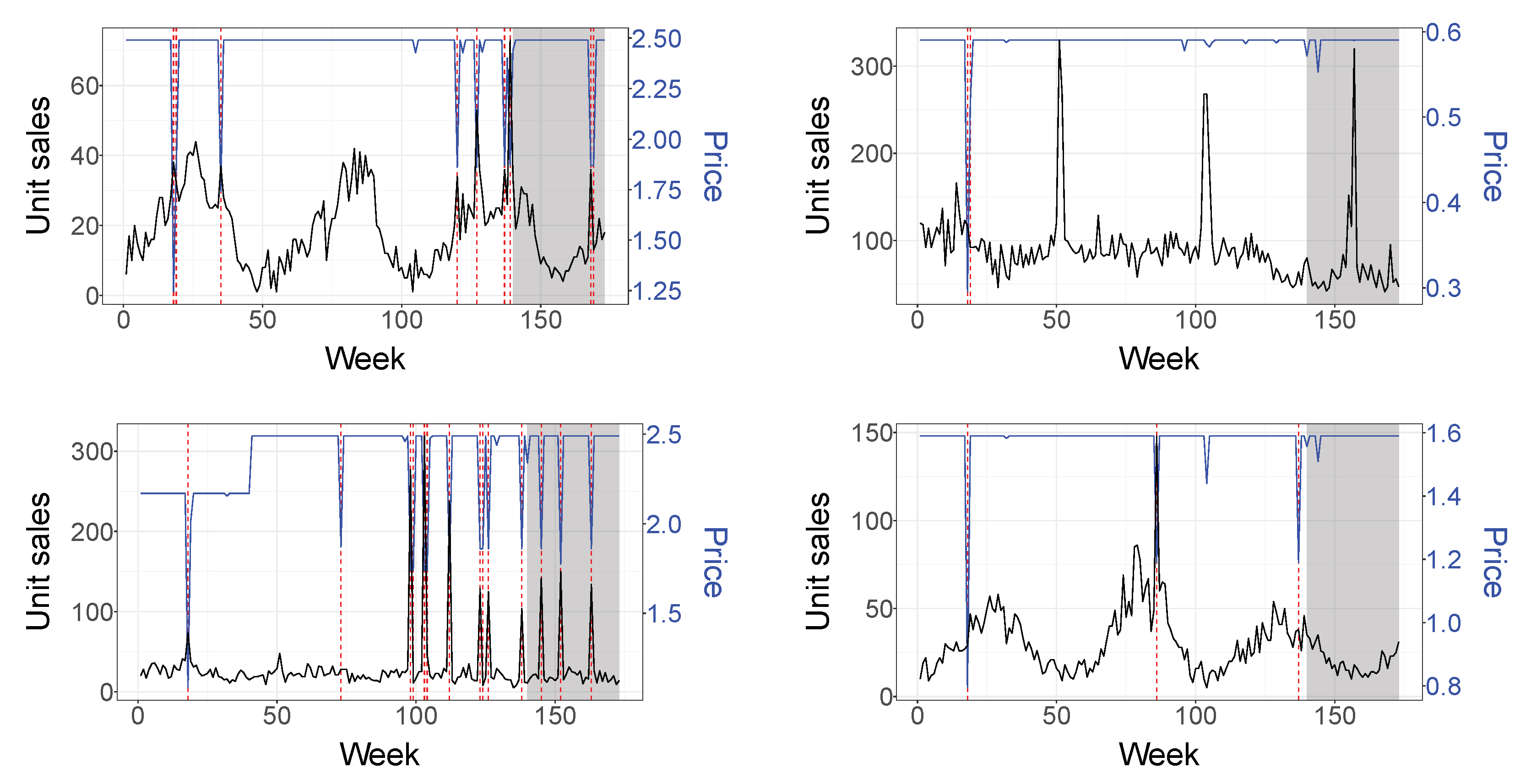
Figure 1 plots the unit sales, price (in the second axis) and promotional periods (marked with dashed lines) of four typical SKUs. Two show a clear annual seasonal pattern that remains fairly constant during the sampled period. We observe that product sales spikes are associated with price reductions and calendar events such as Easter and Christmas. We also see that some products are heavily promoted, exhibiting high variations on their price while others have few promotions. Therefore, our study considers a wide variety of time series containing different features which are typical of this type of business. Any model needs to take these characteristics into account to effectively forecast the unit sales of each SKU. 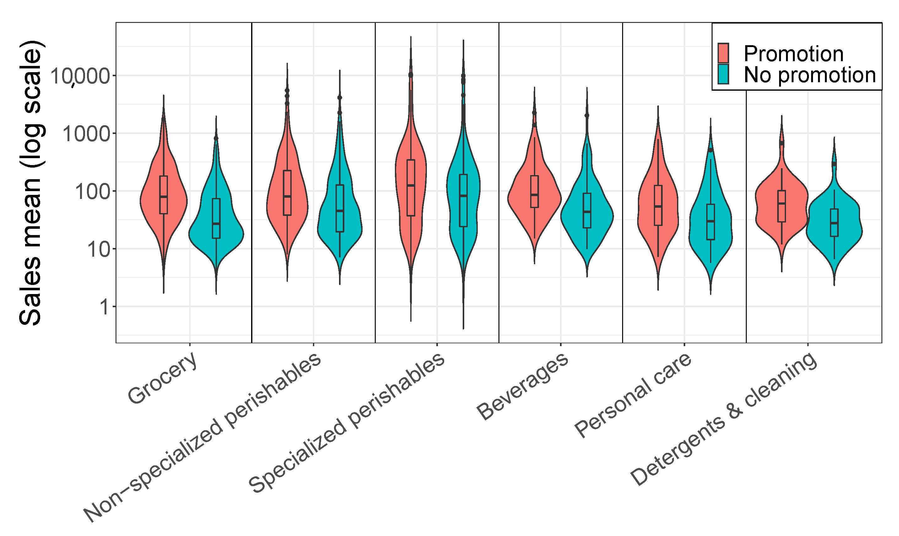Figure 2 shows the impact of promotions on sales. It presents the distribution by category of the average weekly sales on promotional and non-promotional weeks for the selected SKUs, using violin plots, and shows the uplift of the sales on promotional weeks.

Table 2. Statistical description of sales volume on promotional and non-promotional periods for each product category.

Category	Promotion				No Promotion		No. of SKUs
	Mean	Median	Percentage		Mean	Median
Grocery	162.3	79.0	4.9%		63.0	27.1	309
Non-specialized perishables	238.6	80.2	5.5%		144.6	45.3	287
Specialized perishables	492.6	124.1	11.1%		342.0	81.9	193
Beverages	179.7	84.9	8.8%		99.4	43.3	103
Personal care	107.3	53.5	4.9%		61.6	29.8	59
Detergents & cleaning	87.9	60.5	2.7%		40.9	27.8	37

presents statistics of the sales volume with and without promotional activity for each product category during the 173-week period. The sales mean represents the average of the mean weekly unit sales on promotional and non-promotional weeks across all the SKUs of each category. The median is defined similarly. The promotion percentage indicates the percentage of promotional weeks within the 173-week time period for each category. The total number of SKUs in each category is also indicated.

The dataset incorporates 43 covariates and calendar events, some with lead or lagged effects.

• Price and a lag of order 1 (2 inputs).
• Days promoted per week and a lag of order 1 (2 inputs); this variable indicates how many days in the week the SKU is under promotion.
• Last week of the month and a lag of order 1 (24 inputs); this dummy variable captures the end of the month payday effect.
• Binary indicators representing the following calendar events (15 inputs): New Year’s Day, Carnival and the week before, Good Friday and Easter and the week before, Freedom’s Day, Labor’s Day, Corpus Christi week, Portugal’s day, Assumption Day, Republic’s day, All Saints’ Day, Restoration of the Independence, Christmas and the week before.

A logarithmic transformation of the sales time series is used, which helps model multiplicative effects of the aforementioned variables (proportional uplift of sales). At the end the logged target is transformed back to its original units. This transformation is not applied in the case of TBATS, since it already incorporates a Box-Cox transformation.

4.2. Evaluation Design

We evaluate the performance of our models using a rolling forecasting origin scheme. By increasing the number of forecast errors available, we increase the confidence in our findings and facilitate statistical testing. The use of a rolling origin design ensures robustness in the results. We start with a training set containing the first 139 weeks and generate 1- to 13-weeks ahead forecasts for each of the 988 SKUs. The training set is then expanded by one week and the process is repeated until week 160 giving a total of 22 forecast origins. At each forecast origin the models are re-specified automatically using the updated training data. The price and promotional plans are assumed known in the test set, as they are part of the retailer’s marketing strategy. We consider different forecast horizons $H=\{1,1-4,5-8,9-13,1-13\}$ in the comparison to take into account the different ordering and planning periods the retailer faces in practice.

We use two error measures, the Mean Absolute Scaled Error (MASE) [66] and the Root Mean Squared Scaled Error (RMSSE) [17]:

$$\begin{array}{c}{\mathrm{MAE}}_{H,s,k}=\frac{1}{H_2-H_1+1}\sum _{h=H_1}^{H_2}\left|y_{h,s,k}-{\widehat{y}}_{h,s,k}\right|,\end{array}$$

(4)

$$\begin{array}{c}{\displaystyle {\mathrm{MASE}}_{H,s}=\frac{1}{K}\sum _{k=1}^K\frac{{\mathrm{MAE}}_{H,s,k}}{\frac{1}{M-1}{\sum }_{t=2}^M\left|y_{s,k,t}-y_{s,k,t-1}\right|},}\end{array}$$

(5)

$$\begin{array}{c}{\mathrm{MASE}}_H=\frac{1}{S}\sum _{s=1}^S{\mathrm{MASE}}_{H,s},\end{array}$$

(6)

$$\begin{array}{c}{\mathrm{MSE}}_{H,s,k}=\frac{1}{H_2-H_1+1}\sum _{h=H_1}^{H_2}{\left(y_{h,s,k}-{\widehat{y}}_{h,s,k}\right)}^2\end{array}$$

(7)

$$\begin{array}{c}{\displaystyle {\mathrm{RMSSE}}_{H,s}=\sqrt{\frac{1}{K}\sum _{k=1}^K\frac{{\mathrm{MSE}}_{H,s,k}}{\frac{1}{M-1}{\sum }_{t=2}^M{\left(y_{s,k,t}-y_{s,k,t-1}\right)}^2}},}\end{array}$$

(8)

$$\begin{array}{c}{\mathrm{RMSSE}}_H=\frac{1}{S}\sum _{s=1}^S{\mathrm{RMSSE}}_{H,s},\end{array}$$

(9)

where $y_{h,s,k}$ is the $h\mathrm{th}$ observed value in the forecast horizon H of the SKU $s=1,\dots ,S$ at the $k=1,\dots ,K$ forecast origin, and ${\widehat{y}}_{h,s,k}$ is the corresponding forecast. Once the Mean Absolute Error (MAE) and Mean Squared Error (MSE) are calculated, they are summarised across forecast origins and then across SKUs. Both MASE and RMSSE are scale-independent and hence suitable for comparing the forecasts across multiple products of different scales and units. This is achieved by scaling the forecasts errors by the MAE or MSE of the 1-step ahead in-sample naïve forecast errors, to match the absolute or quadratic loss of the numerator [67]. Squared errors favour forecasts that track the mean of the target series, which is influenced by the various special events and promotions, while absolute errors favour forecasts that track the median of the target series and hence focus on the structure of the data.

We can also use the MAE and MSE errors to perform tests on the statistical significance of any reported differences. To this end we use the Multiple Comparison with the Best (MCB) test, advocated by [68]. This is a restricted version of the non-parametric Nemenyi test [69], focusing only on testing the best performing model against the rest. The test is implemented using the nemenyi() function of the R package tsutils [70]. Finally, as part of the testing, we also report mean ranks of the various forecasts.

4.3. Evaluated Methods

We implement the models described in Section 3 with the proposed modifications.

Table 3. Models used in the analysis.

Model Name	Seasonality		Covariates
	Usual	Trigonometric	Raw	PCA
Univariate
ES	✓
TBATS		✓
ARIMA	✓
RegARIMAF		✓
Ridge	✓
RidgeF		✓
With explanatories
ESXPC	✓			✓
PCRegARIMA	✓			✓
PCRegARIMAF		✓		✓
RidgeX	✓		✓
RidgeFX		✓	✓

summarises the model settings, listing the names that will be used in the evaluation. In the table some combinations are omitted. We do not model ES with trigonometric seasonality, as TBATS is used. The latter cannot be readily modified to include explanatory variables. We also do not provide ES and ARIMA with raw explanatory variables, as the number of variables is far too great to reliably estimate the models.

For autoregressions in Ridge we include a combination of up to 5 non-seasonal and 1 seasonal lags, following the recommendation by [59] of using a relatively small number of lags, similarly to ARIMA. For the ES we use the es() function from the R package smooth [71]. The tbats() function from the R package forecast [72] is used to obtain the forecasts for the TBATS model. For the ARIMA we use the auto.arima() function from the same package. For Ridge we use the cv.glmnet() function from the R package glmnet. Finally, all the analysis was done in R [73].

4.4. Results

Table 4. Forecasting performance of the models for all forecast horizons (22 forecast origins).

	Model	$\mathit{H}=1$	1–4	5–8	9–13	1–13
MASE
	RidgeX	0.793	0.822	0.881	0.932	0.883
	PCRegARIMAF	0.795	0.833	0.883	0.929	0.886
	PCRegARIMA	0.804	0.834	0.894	0.942	0.894
	RidgeFX	0.792	0.827	0.898	0.960	0.900
	ESXPC	0.797	0.834	0.904	0.966	0.906
	Ridge	0.894	0.924	0.982	1.035	0.985
	ARIMA	0.908	0.936	0.992	1.040	0.993
	RegARIMAF	0.900	0.933	0.993	1.044	0.994
	TBATS	0.906	0.940	0.998	1.048	0.999
	RidgeF	0.896	0.933	1.009	1.079	1.012
	ES	0.904	0.944	1.018	1.081	1.019
RMSSE
	RidgeX	0.767	0.792	0.825	0.852	0.839
	PCRegARIMAF	0.767	0.820	0.830	0.850	0.854
	PCRegARIMA	0.770	0.799	0.836	0.856	0.847
	RidgeFX	0.762	0.788	0.822	0.854	0.837
	ESXPC	0.764	0.804	0.844	0.872	0.858
	Ridge	0.883	0.910	0.941	0.966	0.955
	ARIMA	0.895	0.922	0.957	0.980	0.970
	RegARIMAF	0.886	0.915	0.947	0.969	0.960
	TBATS	0.888	0.918	0.950	0.976	0.964
	RidgeF	0.876	0.905	0.945	0.981	0.961
	ES	0.894	0.929	0.975	1.006	0.988

summarises the forecasting performance of the various models across all SKUs with respect to the different forecast horizons and error metrics. The best performing model in each column (horizon) is highlighted in boldface. The results are grouped by models with and without covariates, and the rows within each group are sorted by the MASE overall performance.

We highlight some key observations in the table. First, irrespective of the error measure and the horizon, models with covariates perform substantially better. Both PCA and shrinkage are useful and result in gains in forecast accuracy in the order of 10% over the univariate benchmarks. This is expected given the importance of special events, price information, and promotions in retail forecasting. Second, Ridge regression models perform very well overall, and particularly when explanatory variables are available to them. Third, the usefulness of the trigonometric representation depends on the model and error metric. Fourth, the results between MASE and RMSSE differ, which is unsurprising since the error measures focus on different parts of the distribution of the target variable.

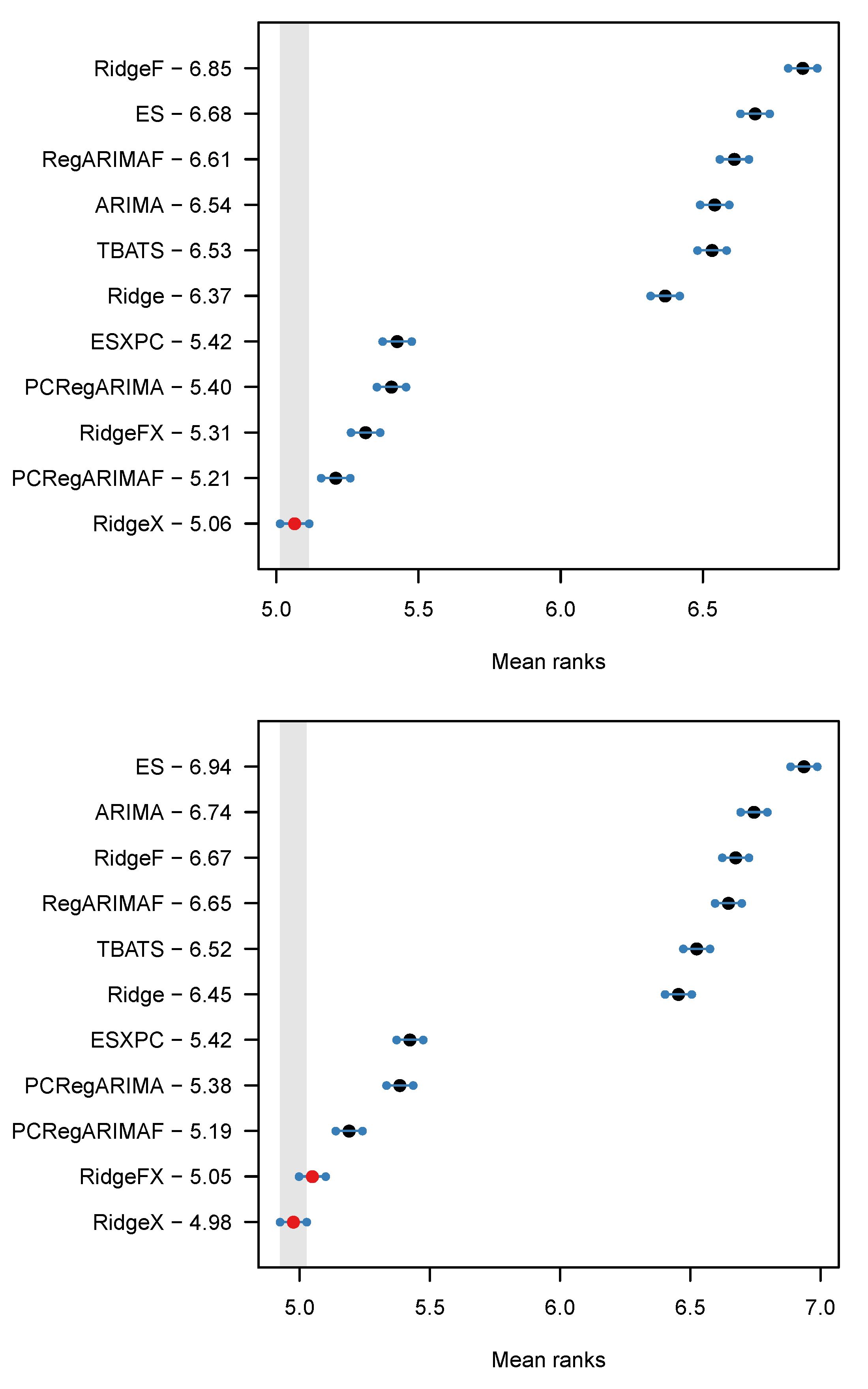
To better compare the models we provide in Figure 3 the models’ mean rank and the results of the MCB test at a 5% significance level, for the horizon 1–13. The forecasts are ranked by their mean rank, which is reported next to their name. The best performing forecasts are at the lowest of the plot and surrounded by a greyed area. For any other forecasts overlapping this area there is no evidence of statistically significant differences. The lines surrounding the forecasts are the critical distances of the Nemenyi test, which function in the same way. The horizontal axis plots the mean rank of the forecasts. For both error measures, RidgeX ranks first. The difference in the top ranking between Table 4 and Figure 3 is attributed to the distribution of the forecast errors, as the mean rank is non-parametric and therefore resilient against outlying errors. Again, we find that models that include the covariates perform best. There is evidence that including these with a shrinkage estimator performs better than using PCA to compress them, although the PCRegARIMAF remains a strong contender. ESXPC trails other models with covariates, yet is substantially better than any of the univariate benchmarks. Last but not least, for almost all of the reported differences there is evidence that they are statistically significant. The results for the other forecast horizons differ slightly, but the key conclusions remain the same, with evidence of significant differences between most cases. We return to the relative performance of PCA and shrinkage estimators when we analyse the results for promotional and non-promotional periods separately.

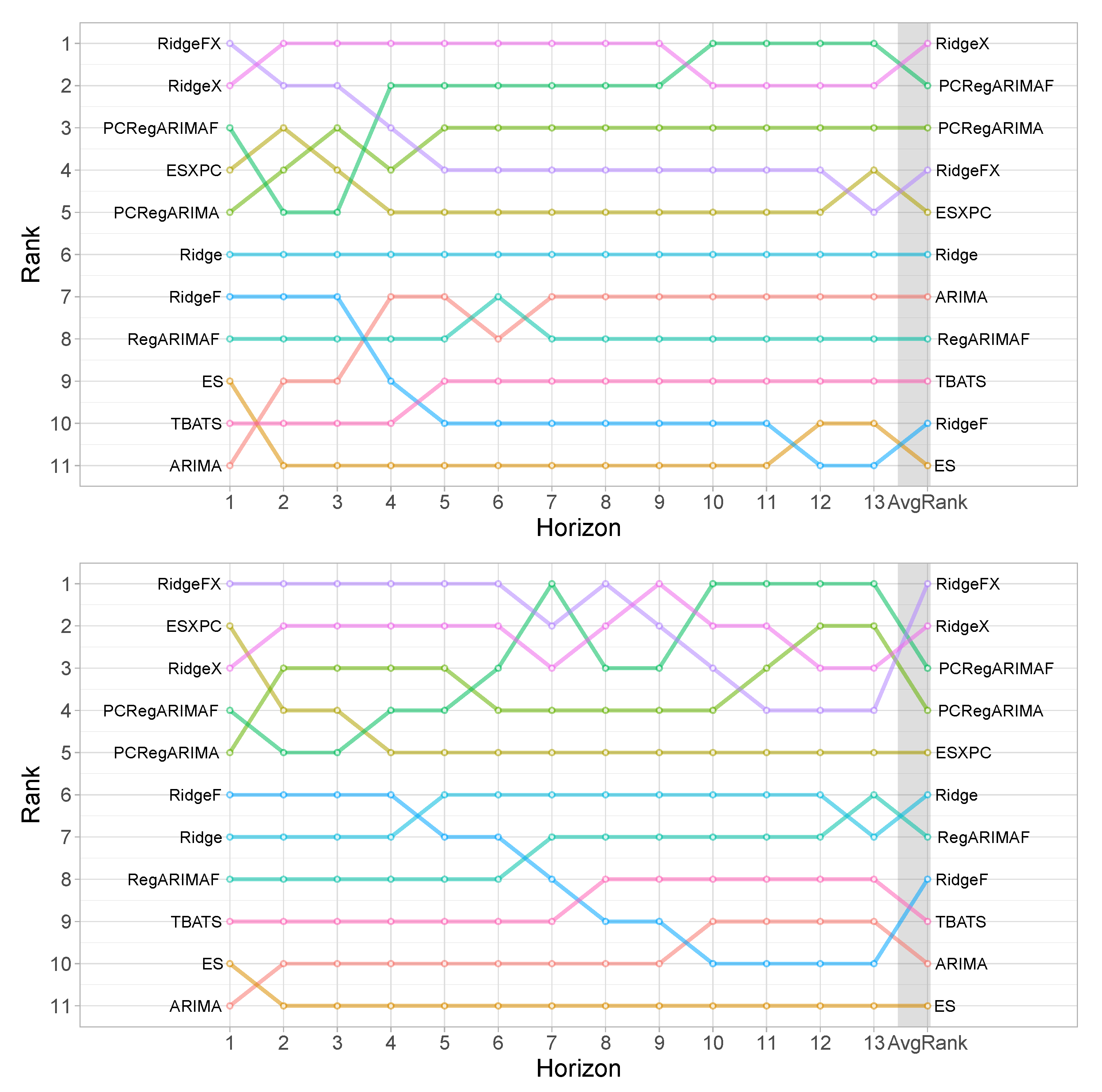
Figure 4 provides the ranking of the models for the various forecast horizons separately. This provides some interesting insights in terms of the progression of the forecasting performance. We observe that in all cases the models with the covariates rank better than the univariate benchmarks. Notably, PCRegARIMAF performs better for longer-term forecasts, for both MASE and RMSSE. So far we have observed a difference in the performance of RidgeX and RidgeFX. This difference becomes clearer when we track the ranking across horizons. In both cases, RidgeFX performs better for short horizons. This is in agreement with the summary statistics in Table 4. The same behaviour is observed for the univariate counterparts, Ridge and RidgeF. This is in contrast to the results for ARIMA in terms of using trigonometric seasonality or not, and arguably the same can be said for the performance between ES and TBATS, with the latter performing better for longer horizons.

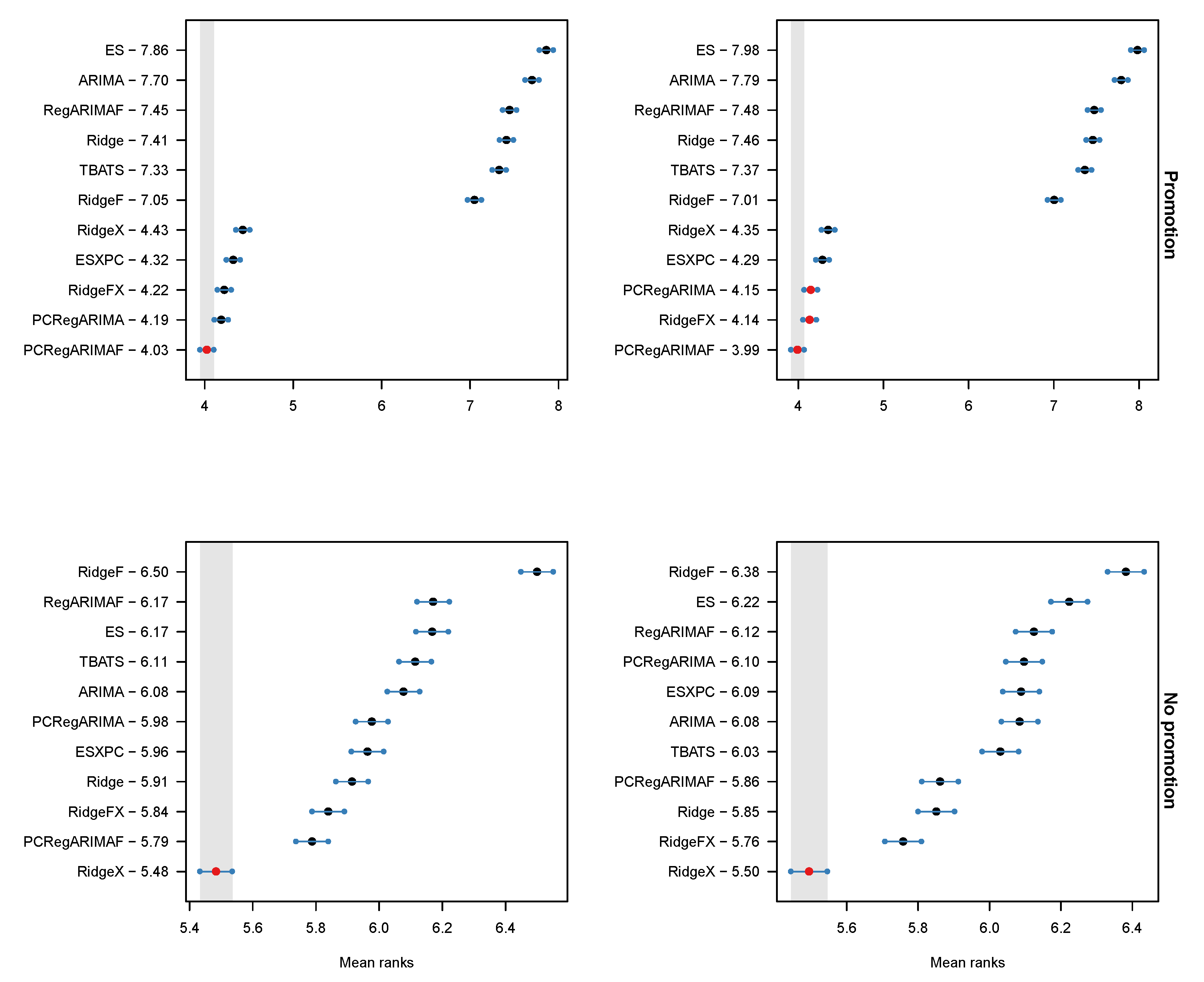
Next, we examine the forecast accuracy for promotional and non-promotional periods separately.

Table 5. Model’s forecasting performance on promotional and non-promotional periods, for the horizon 1–13.

Model	Promotion		No Promotion
	MASE	RMSSE	MASE	RMSSE
RidgeX	3.148	2.096	0.742	0.632
PCRegARIMAF	2.947	2.031	0.754	0.652
PCRegARIMA	2.865	1.937	0.762	0.658
RidgeFX	3.011	2.006	0.763	0.638
ESXPC	2.924	1.982	0.772	0.666
Ridge	4.181	2.667	0.762	0.640
ARIMA	4.191	2.683	0.774	0.661
RegARIMAF	4.173	2.665	0.776	0.651
TBATS	4.174	2.667	0.782	0.659
RidgeF	4.091	2.606	0.797	0.657
ES	4.257	2.726	0.798	0.677

presents the MASE and RMSSE for the horizon 1–13, with the first two columns referring to the promotional case, and the latter two to the non-promotional. At each column the best performing forecast is highlighted in boldface. The table is supplemented by Figure 5 that provides the Nemenyi test results. The striking difference is that when we focus on the promotional periods the PCRegARIMA and PCRegARIMAF perform very well, and in the case of MASE the former significantly outperforms all RidgeFX and RidgeX. Notably, the performance of ESXPC that relies on PCA to encode the coviariates becomes more competitive as well. The opposite is true for the non-promotional periods, which align better with the discussion so far, with RidgeX significantly outperforming all alternatives.

Building on this, we argue that shrinkage estimators deal best with capturing the overall structure of the time series, but on the other hand can over-shrink the effect of promotions. On the other hand, PCA does not impose this shrinkage and therefore performs better during promotional periods, matching the conclusions by [1,11]. Note that the Ridge regression remains competitive, and for RMSSE there is no evidence of significant differences between RidgeFX and the two ARIMA specifications with PCA encoded covariates. Therefore, we argue that as long as the promotional intensity is not very high (as is the case here, see Table 2) the shrinkage estimators provide a simple solution across all promotional and non-promotional periods. If the promotional intensity becomes very high then PCA should be considered.

4.5. Discussion

Overall, we see that the models with covariates outperform their counterparts without covariates across all the forecast horizons, according to both accuracy measures used, in line with the findings of [17]. These findings confirm our initial claim that the inclusion of the main drivers which affect demand at the store level always improves accuracy.

In terms of how to best include covariates we find that in agreement with the literature [1,11,37] both work well to incorporate the rich information available. When promotions are dominant then PCA encoding is beneficial. However, to make the PCA-based models transparent to the users, the principal components need to be remapped to the raw explanatory variances so that the respective coefficients can be inferred. This is not necessary with shrinkage estimators, that perform well overall, and can be a desirable solution when the promotional intensity is not very high.

In terms of the use of trigonometric seasonality, the results are mixed, but again in some agreement with past literature [33,63,64]. Shrinkage estimators are able to introduce sparsity as needed, through the specification of the $\lambda$ hyper-parameter. Therefore, the trigonometric representation is not beneficial. In fact, we find that the trigonometric representation performs relatively poorly for longer-term forecasts. Considering that all models are optimised on one-step-ahead errors, then we can argue that this indicates that RidgeF and RidgeFX in fact have overfitted to the data more than their counterparts Ridge and RidgeX, with better performance around for short-term forecasts, and vice versa for the longer term. On the other hand, for ARIMA that contains no shrinkage, the trigonometric seasonality is beneficial, with increasing relative performance in the long term. Therefore, we conclude that the performance of the trigonometric encoding is estimator dependent.

Furthermore, it is interesting to note that all models used here are fairly transparent, in that one can infer the effect of specific covariates on the sales of each SKU, and potentially use that to optimise the pricing and promotional strategy [39]. As our models were estimated after a logarithmic transformation of the data, any coefficients can be interpreted as elasticities and inform marketing activities, beyond the benefit of having accurate forecasts for operations, such as for inventory planning.

In this study, we have not considered ML and Artificial Intelligence (AI) methods, as this was not compatible with the objectives of our evaluation. Similarly, we excluded using more complex combination schemes of models, for example as in [11]. Although one can infer the impact of specific covariates, the calculations involved are substantially more cumbersome, detracting from the intelligibility of the models and would limit the ability of sales forecasters to inject expert information [31,42] and add substantially to the computational cost, a limitation that remains for forecast combination approaches in the retailing context due to the number of time series involved.

At the onset of this work, we argued that computational simplicity is paramount for retail forecasting, due to the scale of the problem. Some of the models evaluated here are arguably complex when it comes to the formulation, yet with the exception of TBATS and the benchmark ES that need to estimate a substantial number of seasonal parameters, the rest of the models are relatively small and quick to estimate, if the appropriate form is already known. For some of the more successful models, the latter is not necessary. Both RidgeX and PCRegARIMAF are fast to specify. For Ridge regression we have efficient algorithms to optimise it [74]. For PCRegARIMAF we provide a methodology to efficiently compress covariates, model seasonality, and identify the ARMA orders. Therefore, our study helps identify a number of forecasting models that can handle covariates, forecast accurately, are computationally efficient, and allow users to extract the impact of the promotional effects.

5. Conclusions

Demand forecasting at Store × SKU level is a complex problem mainly due to the requirements imposed by large retailers. A forecasting system should include a great variety of drivers that affect SKU demand at store level, such as calendar events and promotional information. Additionally, the forecasts are needed for a large number of products and consequently, the forecasting process must be automated, reliable and computationally efficient.

In this study, we design novel approaches to forecast retailer product sales taking into account the main drivers that affect SKU demand at store level. We propose a feasible solution to include all relevant effects, including promotions, into the statistical ARIMA and ES models based on principal components selected automatically, which prevents overfitting. We also propose an automatic approach to model the short-term dynamics and the seasonality of the demand with Ridge regression. Both, stochastic seasonality represented by seasonal lags, and deterministic seasonality included as Fourier terms, are implemented for comparison.

Using a diverse retail dataset, we compare the forecast performance of our proposed models over several forecast horizons based on two error measures. The forecasting performance results enable us to conclude that the models with covariates outperform their counterparts without covariates across all the forecast horizons, according to both metrics used. These findings confirm that the inclusion of the main drivers which affect demand at store level can significantly impact the performance of forecasting methods, but also that the proposed modelling approach can take advantage of them.

RidgeX is generally the most accurate out of all competing models. This suggests that shrinkage is relatively more accurate in estimating effects from covariates. Nonetheless, when we focus on the forecast performance solely for promotional periods the PCA based models perform best. This finding helps to synthesise different results from the literature that advocates for both approaches. Furthermore, the shrinkage based models enable inference directly, if this is needed. We found a distinct difference in the behaviour of trigonometric seasonality compared to more standard approaches such as stochastic seasonality. It was not beneficial when a shrinkage estimator was used but provided significant accuracy gains otherwise. This research helps to clarify some of the modelling preferences for retail forecasting, as most of the past contributions in the literature have focused on demonstrating the performance of a single, often novel, algorithm. Our work consolidates some of this research. However, as we were motivated by computational efficiency we did not consider ML and AI approaches. The investigated forecasting approaches have the advantage of being relatively transparent against ML and AI methods. The latter do not inform the users on estimated promotional effects that can be useful inputs for promotional and pricing plans. Moreover, for these approaches to become useful in such a setting, they have substantial computational and data requirements.

This study has several implications for practice. Retailers, and in particular supermarkets like the one in our case study, have to face the challenge of incorporating extensive promotional information into their models, along with other covariates. This is often done inefficiently resulting in miscalibrated models, the forecasts of which often require substantial manual adjustments by demand planners [42]. Our recommended models can be automatically calibrated for each item, including relevant effects. On the one hand, this provides gains in forecast accuracy. On the other hand, the models are sufficiently transparent to support promotional planning activities and can increase the trust of users towards the models [31]. For these benefits to be realisable the recommended models need to be relatively easy to implement. Depending on the existing forecasting support system, adopting the dimensionality reduction or shrinkage route may be more attractive. The generation of the additional features for the proposed seasonality encoding does not need any specialised statistical software. If the existing forecasting support system incorporates shrinkage estimators, then the use of the proposed ridge regression becomes straightforward once the additional features have been generated. When this capability is not available, the PCA preprocessing of the input variables can be done prior to incorporation in standard statistical models, which are widely available. If an in-house data science team is available, then either models can be implemented fairly easily relying on a stack of commonly available modelling steps. We argue that this ease of implementation is one of the biggest benefits of our models. Nonetheless, considering the implementation dimension, it points to the relevant question of software interface design. This is beyond the scope of this study, but we recognise its importance for users to get the maximum benefit of the proposed models, both in terms of increasing their trust in them, but also in terms of gaining market insights with benefits beyond forecasting. The design of an appropriate interface for forecasting support systems for retailing remains an interesting direction for future research. In addition, there remains the need to investigate yet more diverse types of promotional information, in particular when we consider how users interact with model forecasts and adjust them to enrich the included information [42].

References

1. Fildes, J.R.T.N.K.R. On the identification of sales forecasting models in the presence of promotions. J. Oper. Res. Soc. 2015, 66, 299–307. [Google Scholar] [CrossRef] [Green Version]
2. Oliveira, J.M.; Ramos, P. Assessing the Performance of Hierarchical Forecasting Methods on the Retail Sector. Entropy 2019, 21, 436. [Google Scholar] [CrossRef] [PubMed] [Green Version]
3. Fildes, R.; Ma, S.; Kolassa, S. Retail forecasting: Research and practice. Int. J. Forecast. 2019, 38, 1283–1318. [Google Scholar] [CrossRef] [Green Version]
4. Seaman, B. Considerations of a retail forecasting practitioner. Int. J. Forecast. 2018, 34, 822–829. [Google Scholar] [CrossRef]
5. Kalyanam, K.; Borle, S.; Boatwright, P. Deconstructing Each Item’s Category Contribution. Mark. Sci. 2007, 26, 327–341. [Google Scholar] [CrossRef]
6. Corsten, D.; Gruen, T. Desperately Seeking Shelf Availability: An Examination of the Extent, the Causes, and the Efforts to Address Retail Out-of-Stocks. Int. J. Retail. Distrib. Manag. 2003, 31, 605–617. [Google Scholar] [CrossRef]
7. Cooper, L.G.; Baron, P.; Levy, W.; Swisher, M.; Gogos, P. PromoCast™: A New Forecasting Method for Promotion Planning. Mark. Sci. 1999, 18, 301–316. [Google Scholar] [CrossRef] [Green Version]
8. Van Donselaar, K.; Peters, J.; de Jong, A.; Broekmeulen, R. Analysis and forecasting of demand during promotions for perishable items. Int. J. Prod. Econ. 2016, 172, 65–75. [Google Scholar] [CrossRef]
9. Pina, M.; Gaspar, P.D.; Lima, T.M. Decision Support System in Dynamic Pricing of Horticultural Products Based on the Quality Decline Due to Bacterial Growth. Appl. Syst. Innov. 2021, 4, 80. [Google Scholar] [CrossRef]
10. European Parliament. Parliament Calls for Urgent Measures to Halve Food Wastage in the EU; Technical Report; European Commission: Luxembourg, 2012.
11. Kourentzes, N.; Petropoulos, F. Forecasting with multivariate temporal aggregation: The case of promotional modelling. Int. J. Prod. Econ. 2016, 181, 145–153, SI: ISIR 2014. [Google Scholar] [CrossRef]
12. Abolghasemi, M.; Beh, E.; Tarr, G.; Gerlach, R. Demand forecasting in supply chain: The impact of demand volatility in the presence of promotion. Comput. Ind. Eng. 2020, 142, 106380. [Google Scholar] [CrossRef] [Green Version]
13. Abolghasemi, M.; Hurley, J.; Eshragh, A.; Fahimnia, B. Demand forecasting in the presence of systematic events: Cases in capturing sales promotions. Int. J. Prod. Econ. 2020, 230, 107892. [Google Scholar] [CrossRef]
14. Holzer, P.S. The effect of time-varying factors on promotional activity in the German milk market. J. Retail. Consum. Serv. 2020, 55, 102090. [Google Scholar] [CrossRef]
15. Verstraete, G.; Aghezzaf, E.H.; Desmet, B. A data-driven framework for predicting weather impact on high-volume low-margin retail products. J. Retail. Consum. Serv. 2019, 48, 169–177. [Google Scholar] [CrossRef]
16. Alon, I.; Qi, M.; Sadowski, R.J. Forecasting aggregate retail sales: A comparison of artificial neural networks and traditional methods. J. Retail. Consum. Serv. 2001, 8, 147–156. [Google Scholar] [CrossRef]
17. Makridakis, S.; Spiliotis, E.; Assimakopoulos, V. M5 accuracy competition: Results, findings, and conclusions. Int. J. Forecast. 2022, 38, 1346–1364. [Google Scholar] [CrossRef]
18. Bojer, C.S.; Meldgaard, J.P. Kaggle forecasting competitions: An overlooked learning opportunity. Int. J. Forecast. 2021, 37, 587–603. [Google Scholar] [CrossRef]
19. Ke, G.; Meng, Q.; Finley, T.; Wang, T.; Chen, W.; Ma, W.; Ye, Q.; Liu, T.Y. LightGBM: A highly efficient gradient boosting decision tree. Adv. Neural Inf. Process. Syst. 2017, 30, 1–9. [Google Scholar]
20. Ma, S.; Fildes, R. Retail sales forecasting with meta-learning. Eur. J. Oper. Res. 2021, 288, 111–128. [Google Scholar] [CrossRef]
21. Nikolopoulos, K.; Petropoulos, F. Forecasting for big data: Does suboptimality matter? Comput. Oper. Res. 2018, 98, 322–329. [Google Scholar] [CrossRef] [Green Version]
22. Fry, C.; Brundage, M. The M4 forecasting competition—A practitioner’s view. Int. J. Forecast. 2020, 36, 156–160, M4 Competition. [Google Scholar] [CrossRef]
23. Gilliland, M. The value added by machine learning approaches in forecasting. Int. J. Forecast. 2020, 36, 161–166, M4 Competition. [Google Scholar] [CrossRef]
24. Bandara, K.; Bergmeir, C.; Smyl, S. Forecasting across time series databases using recurrent neural networks on groups of similar series: A clustering approach. Expert Syst. Appl. 2020, 140, 112896. [Google Scholar] [CrossRef] [Green Version]
25. Januschowski, T.; Gasthaus, J.; Wang, Y.; Salinas, D.; Flunkert, V.; Bohlke-Schneider, M.; Callot, L. Criteria for classifying forecasting methods. Int. J. Forecast. 2020, 36, 167–177, M4 Competition. [Google Scholar] [CrossRef]
26. Smyl, S. A hybrid method of exponential smoothing and recurrent neural networks for time series forecasting. Int. J. Forecast. 2020, 36, 75–85, M4 Competition. [Google Scholar] [CrossRef]
27. Salinas, D.; Flunkert, V.; Gasthaus, J.; Januschowski, T. DeepAR: Probabilistic forecasting with autoregressive recurrent networks. Int. J. Forecast. 2020, 36, 1181–1191. [Google Scholar] [CrossRef]
28. Mancuso, P.; Piccialli, V.; Sudoso, A.M. A machine learning approach for forecasting hierarchical time series. Expert Syst. Appl. 2021, 182, 115102. [Google Scholar] [CrossRef]
29. Makridakis, S.; Spiliotis, E.; Assimakopoulos, V.; Semenoglou, A.A.; Mulder, G.; Nikolopoulos, K. Statistical, machine learning and deep learning forecasting methods: Comparisons and ways forward. J. Oper. Res. Soc. 2022, 0, 1–20. [Google Scholar] [CrossRef]
30. Spiliotis, E.; Makridakis, S.; Kaltsounis, A.; Assimakopoulos, V. Product sales probabilistic forecasting: An empirical evaluation using the M5 competition data. Int. J. Prod. Econ. 2021, 240, 108237. [Google Scholar] [CrossRef]
31. Spavound, S.; Kourentzes, N. Making Forecasts More Trustworthy. Foresight: Int. J. Appl. Forecast. 2022, 66, 21–25. [Google Scholar]
32. Ghysels, E.; Osborn, D.R.; Sargent, T.J. The Econometric Analysis of Seasonal Time Series; Cambridge University Press: Cambridge, UK, 2001. [Google Scholar] [CrossRef]
33. Crone, S.F.; Kourentzes, N. Feature selection for time series prediction—A combined filter and wrapper approach for neural networks. Neurocomputing 2010, 73, 1923–1936. [Google Scholar] [CrossRef]
34. Fildes, R.; Kolassa, S.; Ma, S. Post-script—Retail forecasting: Research and practice. Int. J. Forecast. 2021. [Google Scholar] [CrossRef] [PubMed]
35. Gur Ali, O.; Sayın, S.; van Woensel, T.; Fransoo, J. SKU demand forecasting in the presence of promotions. Expert Syst. Appl. 2009, 36, 12340–12348. [Google Scholar] [CrossRef]
36. Gur Ali, O.; Pinar, E. Multi-period-ahead forecasting with residual extrapolation and information sharing—Utilizing a multitude of retail series. Int. J. Forecast. 2016, 32, 502–517. [Google Scholar] [CrossRef]
37. Huang, S.M.R.F.T. Demand forecasting with high dimensional data: The case of SKU retail sales forecasting with intra- and inter-category promotional information. Eur. J. Oper. Res. 2016, 249, 245–257. [Google Scholar] [CrossRef] [Green Version]
38. Li, K.; Chen, Y.; Zhang, L. Exploring the influence of online reviews and motivating factors on sales: A meta-analytic study and the moderating role of product category. J. Retail. Consum. Serv. 2020, 55, 102107. [Google Scholar] [CrossRef]
39. Fildes, S.M.R. A retail store SKU promotions optimization model for category multi-period profit maximization. Eur. J. Oper. Res. 2017, 260, 680–692. [Google Scholar] [CrossRef] [Green Version]
40. Fildes, R.; Goodwin, P.; Lawrence, M.; Nikolopoulos, K. Effective forecasting and judgmental adjustments: An empirical evaluation and strategies for improvement in supply-chain planning. Int. J. Forecast. 2009, 25, 3–23. [Google Scholar] [CrossRef]
41. Trapero, J.R.; Pedregal, D.J.; Fildes, R.; Kourentzes, N. Analysis of judgmental adjustments in the presence of promotions. Int. J. Forecast. 2013, 29, 234–243. [Google Scholar] [CrossRef] [Green Version]
42. Sroginis, A.; Fildes, R.; Kourentzes, N. Use of Contextual and Model-Based Information in Behavioural Operations. Available SSRN 3466929. 2019. Available online: https://ssrn.com/abstract=3466929 (accessed on 6 December 2022). [CrossRef]
43. Kourentzes, N.; Rostami-Tabar, B.; Barrow, D.K. Demand forecasting by temporal aggregation: Using optimal or multiple aggregation levels? J. Bus. Res. 2017, 78, 1–9. [Google Scholar] [CrossRef]
44. Kourentzes, N.; Barrow, D.; Petropoulos, F. Another look at forecast selection and combination: Evidence from forecast pooling. Int. J. Prod. Econ. 2019, 209, 226–235. [Google Scholar] [CrossRef] [Green Version]
45. Barrow, D.; Kourentzes, N.; Sandberg, R.; Niklewski, J. Automatic robust estimation for exponential smoothing: Perspectives from statistics and machine learning. Expert Syst. Appl. 2020, 160, 113637. [Google Scholar] [CrossRef]
46. Soopramanien, T.H.R.F.D. The value of competitive information in forecasting FMCG retail product sales and the variable selection problem. Eur. J. Oper. Res. 2014, 237, 738–748. [Google Scholar] [CrossRef]
47. Soopramanien, T.H.R.F.D. Forecasting retailer product sales in the presence of structural change. Eur. J. Oper. Res. 2019, 279, 459–470. [Google Scholar] [CrossRef]
48. Rebelo, P.R.N.S.R. Performance of state space and ARIMA models for consumer retail sales forecasting. Robot. Comput.-Integr. Manuf. 2015, 34, 151–163. [Google Scholar] [CrossRef] [Green Version]
49. Oliveira, P.R.J.M. A procedure for identification of appropriate state space and ARIMA models based on time-series cross-validation. Algorithms 2016, 4, 76. [Google Scholar] [CrossRef] [Green Version]
50. Hastie, T.; Tibshirani, R.; Friedman, J. The Elements of Statistical Learning; Springer Series in Statistics; Springer: New York, NY, USA, 1998. [Google Scholar] [CrossRef]
51. Ahrens, N.S.A.D. A hybrid seasonal autoregressive integrated moving average and quantile regression for daily food sales forecasting. Int. J. Prod. Econ. 2015, 170, 321–335. [Google Scholar] [CrossRef]
52. Wang, H.; Li, G.; Tsai, C.L. Regression coefficient and autoregressive order shrinkage and selection via the lasso. J. R. Stat. Soc. Ser. B (Stat. Methodol.) 2007, 69, 63–78. [Google Scholar] [CrossRef]
53. Fildes, R.; Petropoulos, F. Simple versus complex selection rules for forecasting many time series. J. Bus. Res. 2015, 68, 1692–1701. [Google Scholar] [CrossRef]
54. Harvey, A.C. Forecasting, Structural Time Series Models and the Kalman Filter; Cambridge University Press: Cambridge, UK, 1989. [Google Scholar] [CrossRef]
55. Barrow, D.; Kourentzes, N. The impact of special days in call arrivals forecasting: A neural network approach to modelling special days. Eur. J. Oper. Res. 2018, 264, 967–977. [Google Scholar] [CrossRef] [Green Version]
56. Snyder, A.M.D.L.R.J.H.R.D. Forecasting time series with complex seasonal patterns using exponential smoothing. J. Am. Stat. Assoc. 2011, 106, 1513–1527. [Google Scholar] [CrossRef] [Green Version]
57. Ord, J.K.; Fildes, R.; Kourentzes, N. Principles of Business Forecasting, 2nd ed.; Wessex Press Publishing Co.: London, UK, 2017. [Google Scholar]
58. Box, G.E.P.; Jenkins, G.M.; Reinsel, G.C.; Ljung, G.M. Time Series Analysis: Forecasting and Control, 5th ed.; John Wiley & Sons, Inc.: Hoboken, NJ, USA, 2015. [Google Scholar]
59. Hyndman, R.J.; Khandakar, Y. Automatic time series forecasting: The forecast package for R. J. Stat. Softw. 2008, 26, 1–22. [Google Scholar] [CrossRef] [Green Version]
60. Hyndman, R.J.; Koehler, A.B.; Snyder, R.D.; Grose, S. A state space framework for automatic forecasting using exponential smoothing methods. Int. J. Forecast. 2002, 18, 439–454. [Google Scholar] [CrossRef] [Green Version]
61. Hyndman, R.J.; Koehler, A.B.; Ord, J.K.; Snyder, R.D. Forecasting with Exponential Smoothing: The State Space Approach; Springer Series in Statistics; Springer: Berlin/Heidelberg, Germany, 2008. [Google Scholar] [CrossRef]
62. Jolliffe, I. Principal Component Analysis, 2nd ed.; Springer Series in Statistics; Springer: New York, NY, USA, 2002. [Google Scholar] [CrossRef]
63. Miller, D.M.; Williams, D. Shrinkage estimators of time series seasonal factors and their effect on forecasting accuracy. Int. J. Forecast. 2003, 19, 669–684. [Google Scholar] [CrossRef]
64. Kourentzes, N.; Petropoulos, F.; Trapero, J.R. Improving forecasting by estimating time series structural components across multiple frequencies. Int. J. Forecast. 2014, 30, 291–302. [Google Scholar] [CrossRef] [Green Version]
65. Hanssens, D.M.; Parsons, L.J.; Schultz, R.L. Market Response Models: Econometric and Time Series Analysis; International Series in Quantitative Marketing; Springer: New York, NY, USA, 2001; Volume 12. [Google Scholar] [CrossRef]
66. Hyndman, R.J.; Koehler, A.B. Another look at measures of forecast accuracy. Int. J. Forecast. 2006, 22, 679–688. [Google Scholar] [CrossRef] [Green Version]
67. Athanasopoulos, G.; Kourentzes, N. On the evaluation of hierarchical forecasts. Int. J. Forecast. 2022, in press. [Google Scholar] [CrossRef]
68. Koning, A.J.; Franses, P.H.; Hibon, M.; Stekler, H. The M3 competition: Statistical tests of the results. Int. J. Forecast. 2005, 21, 397–409. [Google Scholar] [CrossRef]
69. Hollander, M.; Wolfe, D.A.; Chicken, E. Nonparametric Statistical Methods; John Wiley & Sons, Inc.: Hoboken, NJ, USA, 2015. [Google Scholar] [CrossRef]
70. Kourentzes, N. tsutils: Time Series Exploration, Modelling and Forecasting, R package version 0.9.2; R Foundation for Statistical Computing: Vienna, Austria, 2020. [Google Scholar]
71. Svetunkov, I. Smooth: Forecasting Using Smoothing Functions, R package version 2.4.0; R Foundation for Statistical Computing: Vienna, Austria, 2018. [Google Scholar]
72. Hyndman, R.; Athanasopoulos, G.; Bergmeir, C.; Caceres, G.; Chhay, L.; O’Hara-Wild, M.; Petropoulos, F.; Razbash, S.; Wang, E.; Yasmeen, F.; et al. Forecast: Forecasting Functions for Time Series and Linear Models, R package version 8.15; R Foundation for Statistical Computing: Vienna, Austria, 2021. [Google Scholar]
73. R Development Core Team. R: A Language and Environment for Statistical Computing; R Foundation for Statistical Computing: Vienna, Austria, 2019. [Google Scholar]
74. Friedman, J.H.; Hastie, T.; Tibshirani, R. Regularization Paths for Generalized Linear Models via Coordinate Descent. J. Stat. Softw. Artic. 2010, 33, 1–22. [Google Scholar] [CrossRef]
Figure 1. Time series plot of four typical SKUs. Promotional periods are marked with dashed lines. The test set corresponds to the shaded area.
Asi 06 00003 g001
Figure 2. Distribution of the average weekly sales on promotional and non-promotional weeks by category.
Asi 06 00003 g002
Figure 3. MCB test results at a 5% significance level based on MASE (top) and on RMSSE (bottom).
Asi 06 00003 g003
Figure 4. Models’ rank for each forecast horizon from 1-to 13 weeks ahead and average rank across all horizons based on MASE (top) and RMSSE (bottom).
Asi 06 00003 g004
Figure 5. MCB test results at a 5% significance level based on MASE (left) and on RMSSE (right) for promotional (top) and non-promotional (bottom) periods (forecast horizon 1–13).
Asi 06 00003 g005