1. Introduction
Industries rely heavily on human inspection for product quality assessment, which is time-consuming and costly [
1]. For example, a factory operating 24 h a day with three shifts would require at least three people to inspect product quality. Additionally, inspection accuracy can also be affected by new employees lacking experience and fatigue issues. An automatic inspection system [
2] can provide a solution by reducing costs and time and providing a direct correlation between operational information and product quality [
3]. An automatic inspection system for identifying defects has several benefits, including operating continuously for extended periods, producing consistent results, and functioning in harsh conditions such as high temperatures and dusty environments [
4]. The use of AI in the industrial field has increased in recent years due to advancements in AI methods, open-source frameworks, and decreased development costs; this also eliminates the need for physical computer storage by using the cloud [
5,
6]. The COVID-19 pandemic has also contributed to the shift towards automation as it forced a reduction in the number of employees in factories [
7].
Deep learning is a popular trend in AI for an automatic inspection system in defect inspection [
8]. It is considered a valuable aspect of AI due to its superiority over traditional machine learning methods. Defect inspection using deep learning can effectively identify and classify defects in various materials and products. Deep learning models, particularly convolutional neural networks (CNNs) [
9,
10], are particularly effective at image classification tasks and can be trained to recognize and classify defects based on visual characteristics [
11]. One advantage of using deep learning for defect inspection is that it is more accurate and consistent than traditional methods [
12]. However, some challenges and limitations to using deep learning for defect inspection exist. One of the main challenges is obtaining a large and diverse enough dataset of labeled defects for training the model. Additionally, deep learning models can be computationally expensive to train and deploy, particularly for real-time inspection applications, especially in the real-time inspection of cylindrical shell moving objects [
13,
14].
One of the main challenges in the defect inspection of moving cylindrical shell objects is that the object is in motion during the inspection process [
13]. This can make it difficult to acquire high-quality images or sensor data that can be used for defect detection. Some specific problems include Image blur: When the object is moving, the images captured during the inspection process may be blurred, making it difficult to detect defects accurately [
15]. Sensor data variability: The sensor data collected from a moving object may be more variable than from a stationary object, making it more challenging to train a deep learning model for defect detection [
16]. Occlusion: Moving parts of the object may occlude defects, making them difficult to detect. Vibration: The object’s vibration during the inspection process can make it difficult to acquire high-quality images or sensor data [
17]. Alignment: The object may not be aligned with the sensor during an inspection, making it challenging to acquire accurate images or sensor data. Researchers have proposed various methods to overcome these problems, such as using multiple High-Frame Rate Camera Sensors [
18] and advanced deep-learning architectures [
19].
Fast-speed cameras can be used in the defect inspection of moving cylindrical shell objects by capturing high-speed images of the object as it moves [
20]. These images can then be analyzed to detect defects on the object’s surface. One way to use fast-speed cameras for defect inspection is to capture images of the object at a high frame rate and then use image processing techniques to extract features from the images. These features can then be used to train a deep learning model for defect detection. Another way to use fast-speed cameras for defect inspection is to capture images of the object at a high frame rate and then use motion compensation algorithms to align the images and reduce blur. This can help improve image quality and make it easier to detect defects. Additionally, fast-speed cameras can capture images of the object at multiple angles, which can help to improve the accuracy of defect detection by providing more information about the object’s surface. In summary, fast-speed cameras can be used to capture high-speed images of moving cylindrical shell objects and then use image processing and motion compensation techniques to improve the image quality and detect defects on the object’s surface, and also help to improve the accuracy of the detection by providing more information about the object’s surface. However, employing deep learning on multiple high frame rate cameras (HFRC) causes the need for much computation and decreases deep learning performance, especially in the real-time inspection of moving objects.
In this study, we developed deep learning to assess the quality of cylindrical shell products produced by PT Pindad, Indonesia. The deep learning model received input from three high frame rate camera sensors. The three cameras captured the position of the cylindrical shell objects from the top, longitudinal side, and bottom. High frame rate camera sensors are used because the cameras will capture rotating objects, so the cameras must be able to capture all parts of the object accurately. High frame rate cameras, of course, must be combined with a fast system with minimal delay in terms of hardware and software. Several CNN-based deep learning models were utilized, such as VGG, ResNet, MobileNet v1, MobileNet v2, EfficientNet v1, and EfficientNet v2, to obtain the best performance suitable for the high frame rate camera, high accuracy, and low computation resource for decreasing delay. The deep learning model in this study tested two types of applications, web- and desktop-based, to obtain the lowest computation resources.
2. Materials and Methods
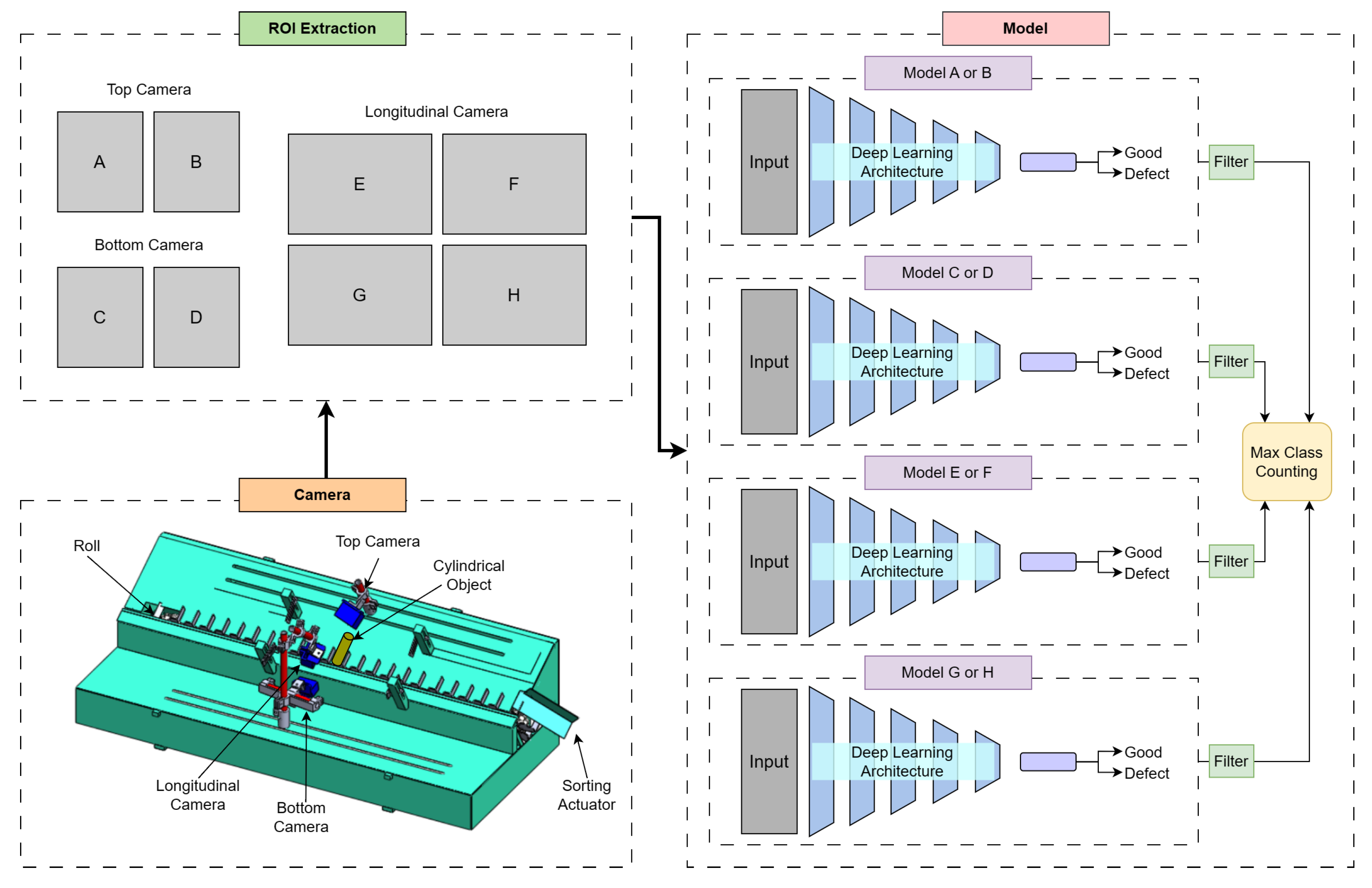
This study proposes a lightweight computing resource framework for high frame rate camera input to obtain high accuracy in the defect inspection of moving cylinder shell objects. The entire process in our system is summarized in
Figure 1. In the initial process, the target object is rolled in a circular motion that requires more than one frame for 360-degree rotation in a conveyor belt. Therefore, it needs more than one frame for each side of the camera. The three high FPS cameras captured all parts of the object with the positions of the top, longitudinal/sides, and bottom of the target. As the conveyor machine moves, the software will process every frame captured by the camera with a built-in deep learning model. The initial stages of processing each frame are image preprocessing, a four-deep learning model, and quality decision-making of rotating objects. In the last conveyor belt, an actuator for filtering a product based on the model results was connected to the decision-making system.
The image preprocessing stage begins with splitting the frame captured by each camera into several parts. The frame captured by the top and bottom cameras was divided into two pieces, while the longitudinal side was divided into four parts. The purpose of the division was to make a square size of frame that can help the deep learning model produce optimal accuracy. The feature extraction stage is performed by the deep learning model automatically. The feature extraction stage aims to capture important information in the input image. After the data from the input image has been obtained, the next step is that the deep learning model generates information on the quality of rotating objects from each frame. For each model frame, two classes of images were applied in this study, i.e., good and defective. The final stage is decision-making based on the quality of the information in each frame. If more than five frames of images on one of the cameras were analyzed as having defective quality, then the cylinder shell object was classified as a defective product.
2.1. Dataset
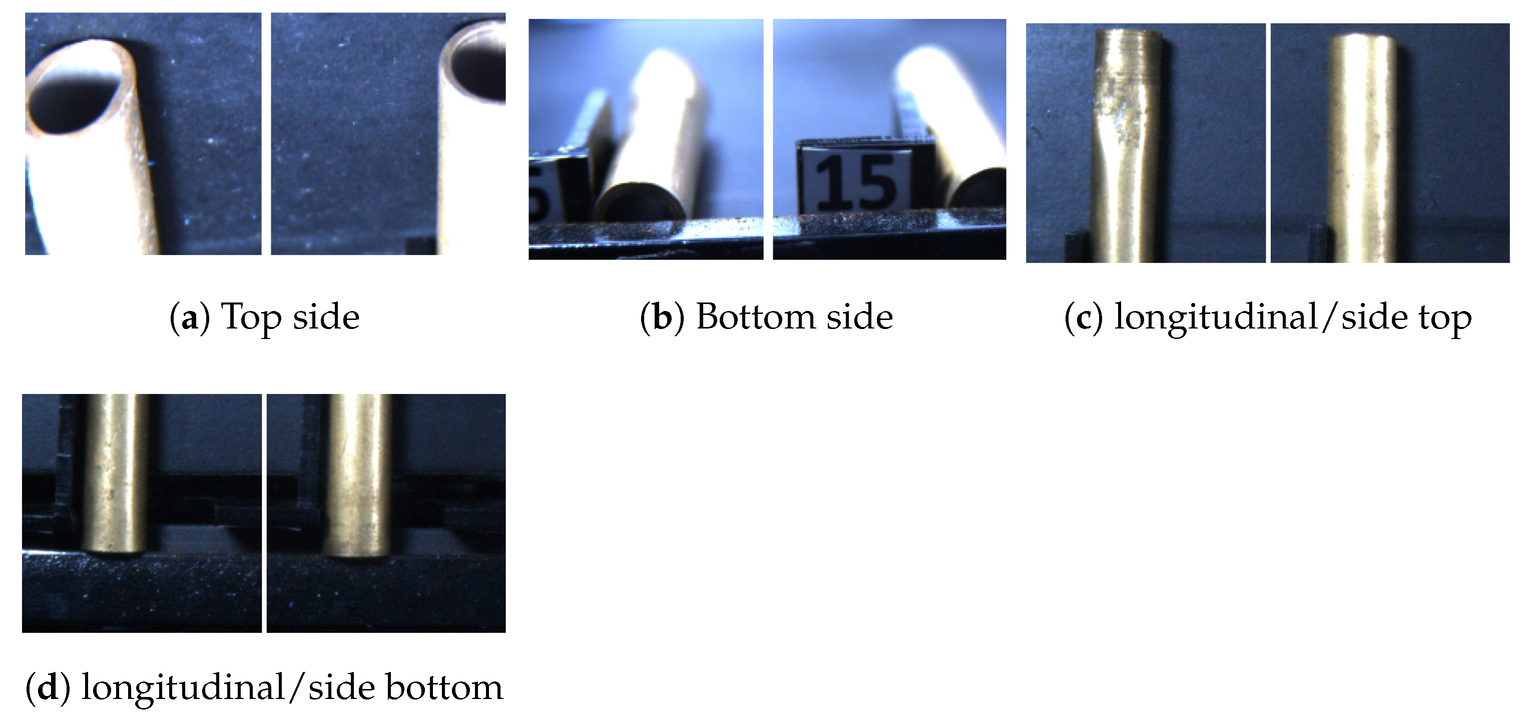
The cylindrical shell object is made of brass and may have defects on the surface and dent on the edges of the holes, as shown in
Figure 2. Therefore, it requires three positioned cameras to find the dent on the surface for the defect class as shown in
Figure 2c left sides. The good cylindrical shell class was a product without any dent in the surface as shown in
Figure 2c right sides. The dataset is not publicly available, and it is recorded directly using a camera with a maximum capacity of 210 FPS to capture each side of a rotating object. The cameras capture the cylinder’s top, longitudinal/side, and bottom sides. The overall position of the camera is on a two-dimensional plane so that it can capture the entire sides simultaneously.
Every movement of the object was captured in a high-quality sensor, which avoided the problem of blurring, occlusion, vibration, and alignment. The movement of the rotating object was driven using a conveyor chain with a speed of 2.5 cm/s.
Figure 2 shows sample datasets from the top, bottom, and longitudinal sides. The object’s color tends to be bluish even though the light around the object is given a white lamp. This occurrence is because we use a camera sensor with a high frame rate that can take 120 FPS. In this study, we used image input with a resolution of 224 × 224 for each frame. The dataset was divided into three parts, namely 80% training data, 20% test data, and 10% validation data from training data.
2.2. Deep Learning Model
In this study, several developed deep learning models were tested, namely VGG, ResNet, MobileNet v1, MobileNet v2, EfficientNet v1, and EfficientNet v2 to find out which model has the best performance. The best of the models is selected as an essential part of the application to serve as the image processing model.
2.2.1. VGG
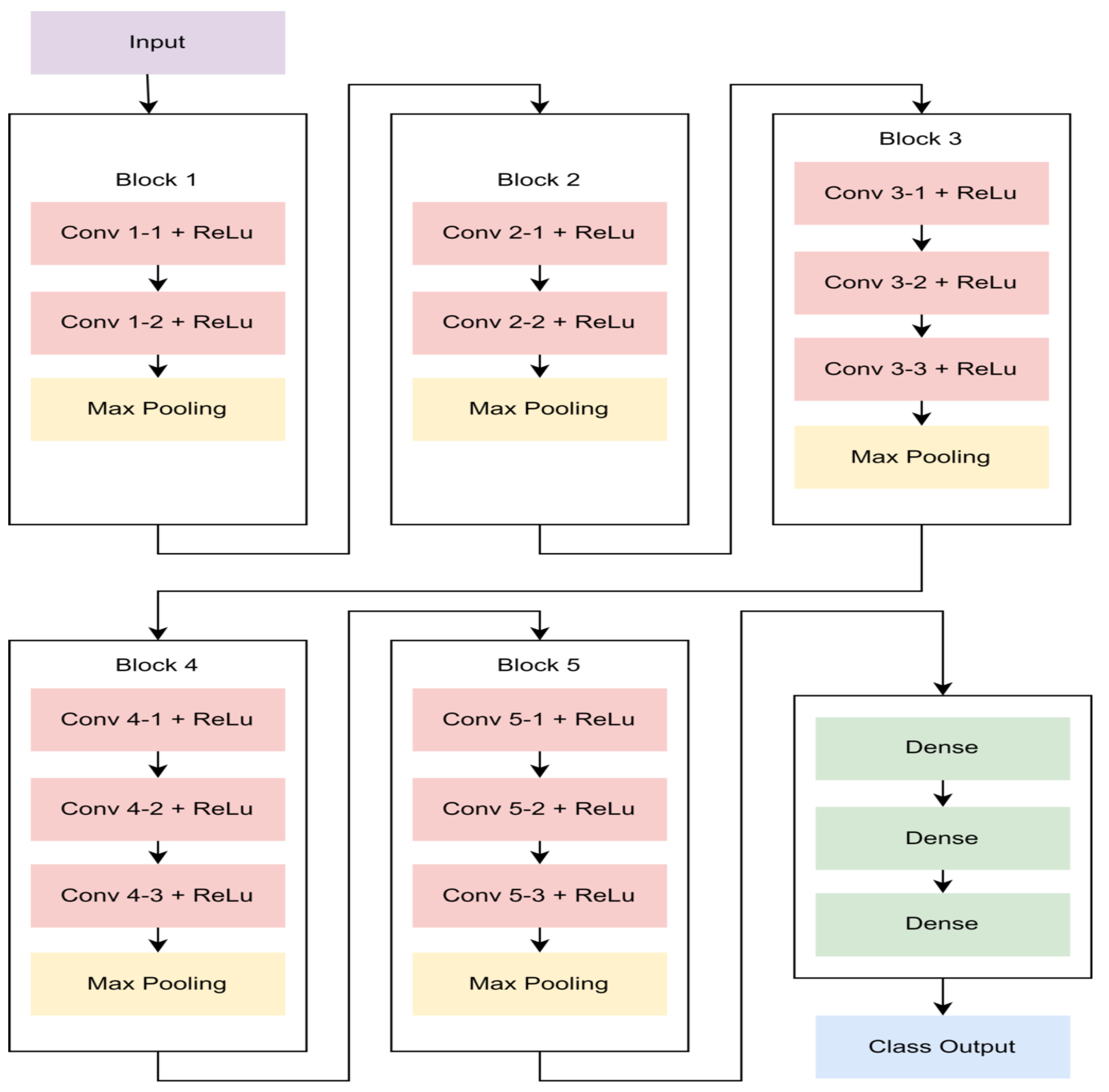
The VGG architecture is a deep learning model inspired by ConvNets [
21]. VGG consists of several ConvNets compiled by increasing the number of ConvNets as shown in
Figure 3. The combination of ConvNets and fully connected layers are arranged from 11 to 19 layers [
22]. In VGG-16, the first two convolutional layers consist of 64 numbers of filters, followed by the two, three, and three convolutional layers having 128, 256, and 512 filters, consecutively.
2.2.2. ResNet
One solution to improve deep learning capabilities is to multiply layers. However, this method has the shortcoming of being easier to lose information with the increased depth of the layers. In addition, other problems that arise are gradients and complexity. Deep learning models that are trained deeper will require longer computational time.
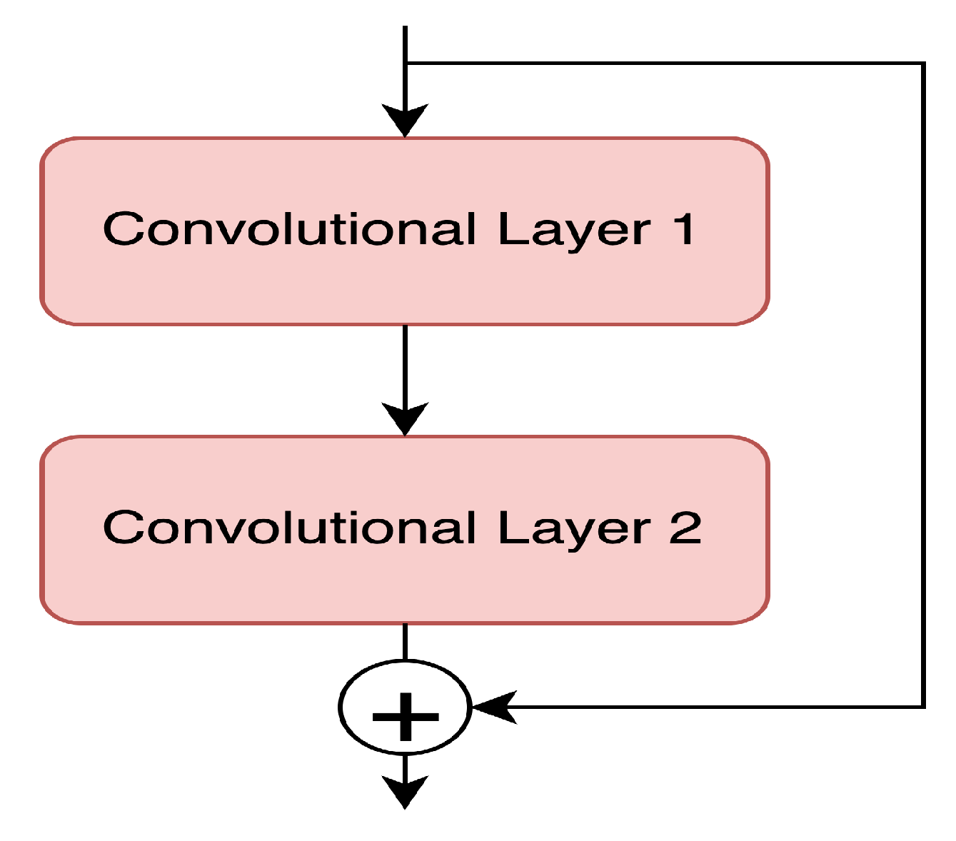
The presence of ResNet in 2015, introduced by [
23] is a deep learning model solution with many layers. ResNet comes with a skip connection that aims to maintain the information or features generated in the previous convolutional layer. In 2022, Saini and Rawat [
24] conducted a study comparing the capabilities of deep learning models using skip connection and without skip connection. Based on the research, ResNet provides higher accuracy, but the arrangement developed does not have too many blocks.
where
y is the resulting value of the summation operation between the output results of two layers.
ResNet is a deep learning model for image classification. This deep learning model is often used as a backbone in various models that are being developed today, such as the backbone for image segmentation models, image classification, detection of objects on images, and others. ResNet is the model with the latest in the form of residual or skip connection. The connection serves to maintain the feature information that has been obtained on the previous layer. The residual network formula is depicted in
Figure 4. ResNet consists of various versions: ResNet consisting of 34 Layers, ResNet consisting of 50 Layers, and ResNet consisting of 101 Layers. According to Sun’s research results, the version of ResNet with a total of 50 layers produces the best performance [
25]. Based on this research, in this study, the pre-trained ResNet model was used as the backbone model of the bottle-neck attention module.
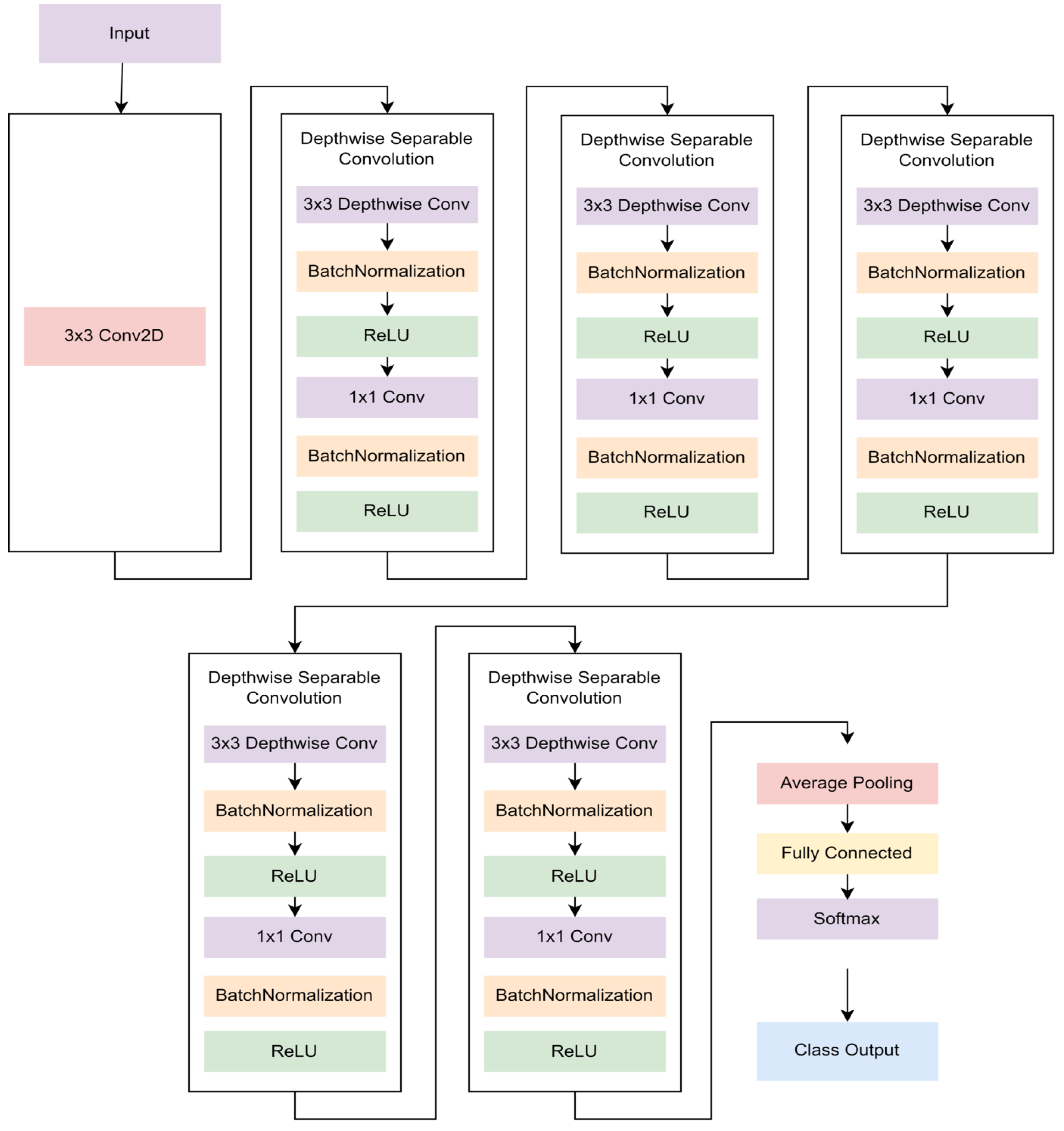
2.2.3. MobileNet
MobileNet was developed by Andrew G. Howard. It is built with depthwise separable convolutions and 1 × 1 pointwise convolution architecture. The purpose of using these two layers in this model is to make the deep learning model light and to speed up the convolution process. These two types of layers cause MobileNet to be used in mobile applications or embedded systems. The two types of layers also make the MobileNet architecture have a smaller number of parameters than other deep learning models but still have good performance [
26]. The MobileNet v1 network is depicted in
Figure 5.
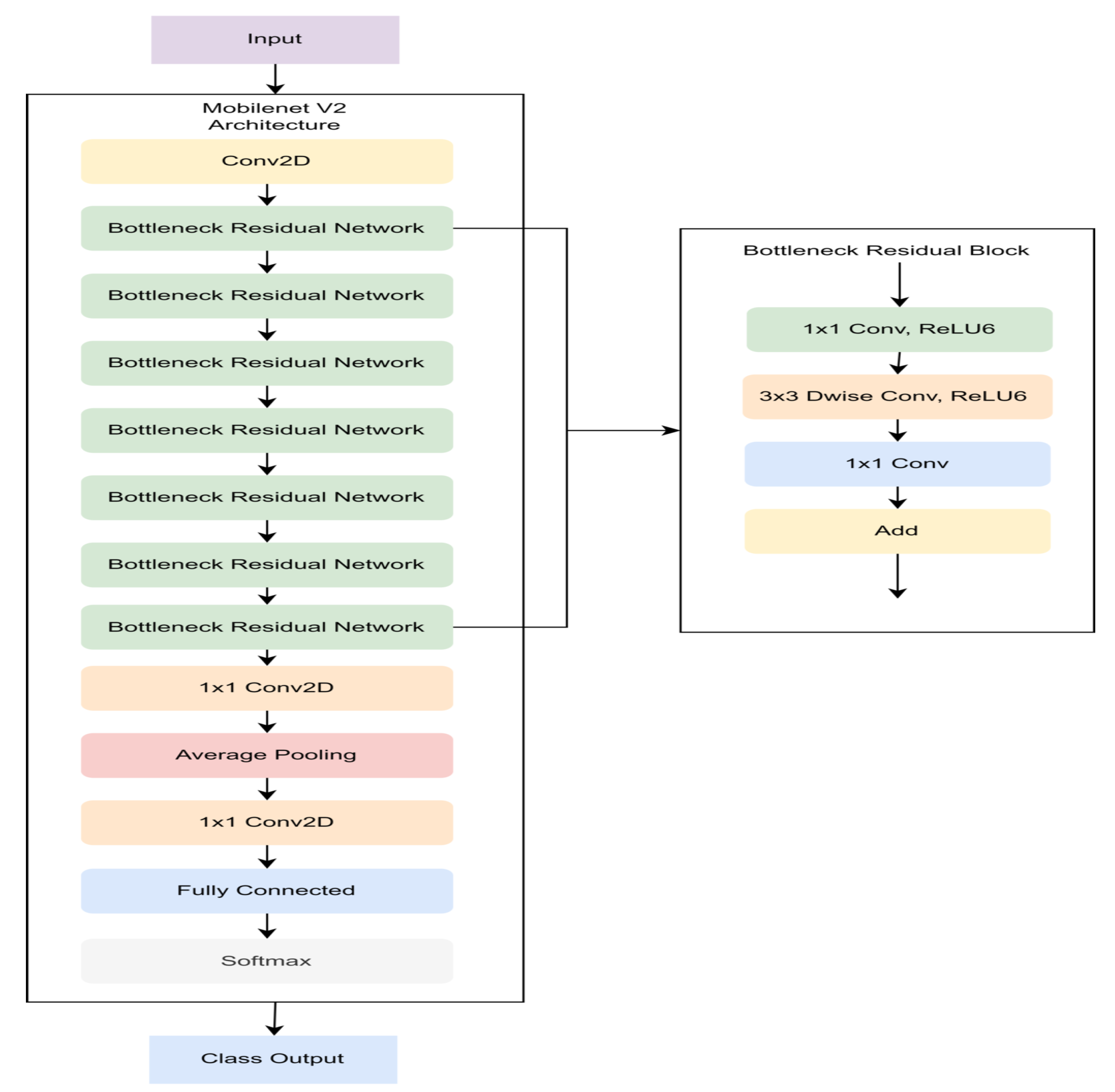
2.2.4. MobileNet v2
Depthwise separable convolution is still the main focus of MobileNet v2 as shown in
Figure 6. The novelty of MobileNet v2 is the addition of layers for extracting features such as linear bottlenecks and residual connections. The bottleneck layer consists of three operations, namely 1 × 1 convolution, 3 × 3 depthwise convolution, and 1 × 1 pointwise convolution. In the first 1 × 1 image convolution, the number of channels is expanded to obtain a complete feature image. The second convolution is the depthwise convolution which serves to filter data. The last convolution is a pointwise convolution that functions to reduce the number of channels but has obtained important information acquired in the previous layer. Each layer in the bottleneck is followed by batch normalization and ReLU6; however, in the last convolution, ReLU6 is not followed because it can eliminate important information. Residual connection aims to preserve the previous layer’s information so that it retains important information [
27].
2.2.5. EfficientNet
The problem of deep learning is inseparable from the problem of speed and accuracy. EfficientNet is a deep learning architecture inspired by MobileNet [
26] and ResNet [
23]. The architecture is developed using a compound model scaling scheme, as shown in
Figure 7. Using a compound scaling model, the efficient net is expanded in the depth, width, and resolution sections. The depth is a model that has a deeper architecture. The width aims to allow the model to capture important information from the inputs, but a wider model will have difficulty capturing high-level information, so a deeper architectural design is needed. Resolution scaling is used so that the model can receive input with a larger resolution so that it can capture high-level information more easily [
28].
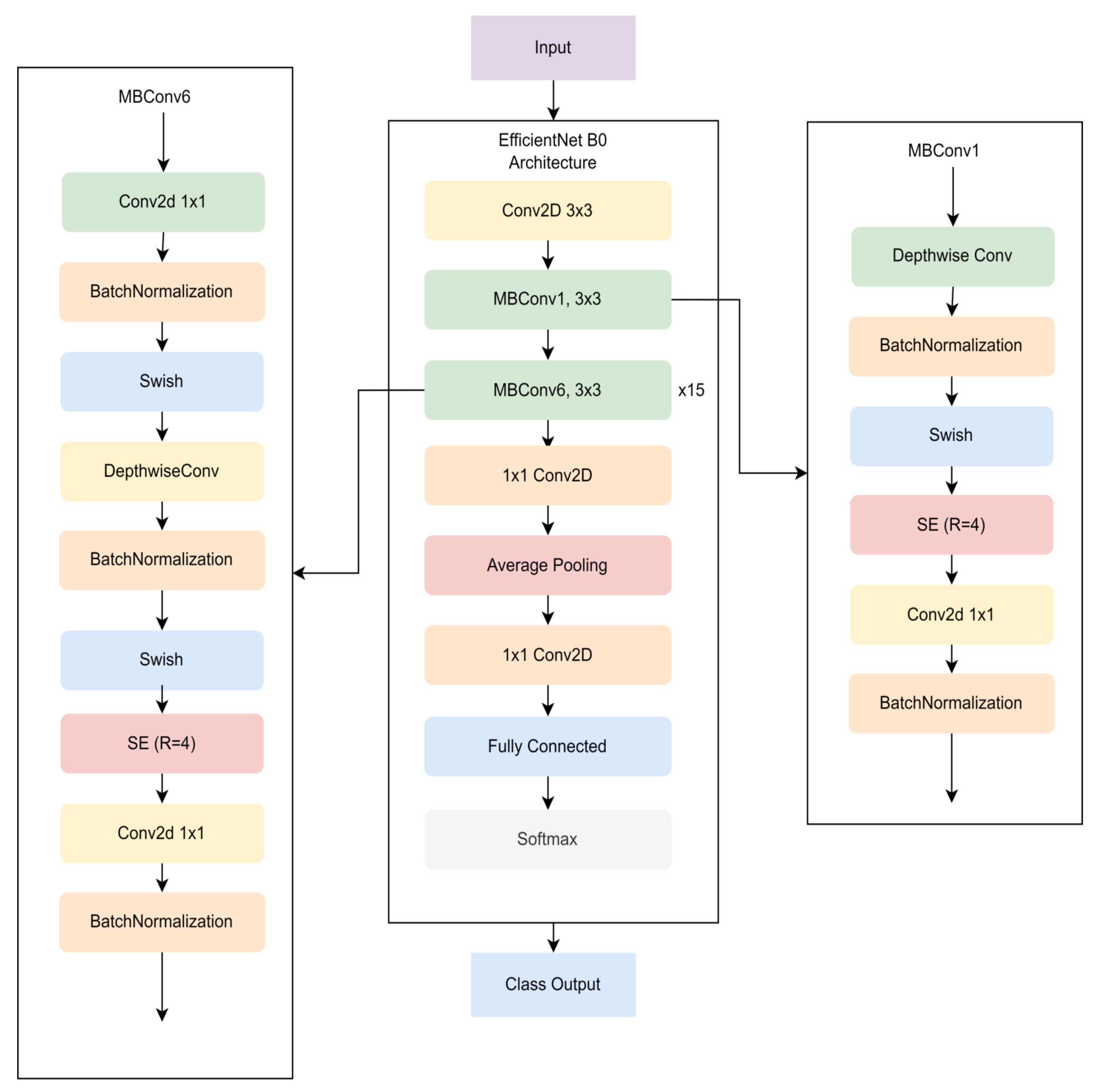
2.2.6. EfficientNet v2
EfficientNet v2 is a development of EfficientNet B0 as shown in
Figure 8. The design of this latest architecture has faster training times and better parameter efficiency [
29]. Using the latest architecture, EfficientNet has 6.8x fewer parameters than its predecessor and is 3x-9x faster during training. In this architecture, EfficientNet uses a new layer design, i.e., Fused MBConv [
30]. The EfficientNet v2 model was designed using NAS Search to obtain the appropriate architecture combination. In the study, there were 1000 model combinations of MBConv and Fused MBConv.
2.3. Tensorflow
Tensorflow is an open-source library that is widely known for solving the problem of deep learning development. The library was released by Google in November 2015 and was developed using the Python programming language [
31]. This library has various deep learning functions to express different deep neural network algorithms. Tensorflow has the advantage of being able to run on multiple platforms, such as desktop, web, mobile, and even embedded systems. TensorFlow can be used for computer vision, speech recognition, information retrieval, and much more research. Tensorflow library processing can be performed using a CPU or GPU.
2.4. OpenCV
OpenCV is an open-source library developed in C++ and Python for image and video analysis, initially introduced by Intel [
32]. The library serves to process images from inputs, processing, and outputs. Information can come from a video file or a camera for streaming. The processing part is used to process images such as object detection, edge detection, or processing images in the form of arrays so that they can be used as input for deep learning libraries such as TensorFlow. The output section displays the results of the OpenCV processing library, and the output can be text or other objects. OpenCV is usually used to process images as input for deep learning models in desktop-based applications.
2.5. Hyperparameter Setting
Each model was divided into three parts: the model for the upper camera sensor, the longitudinal side camera sensor, and the bottom camera sensor. This division was set because the model recognized data patterns more specifically to reduce the occurrence of prediction errors. Based on the division of these models, 18 deep learning models would be formed. The loss function used in this study was categorical cross-entropy, and the cross-entropy loss equation can be seen in Equation (
2).
where
is the label corresponding to the dataset,
is the predicted result of the Softmax activation function, and
n is the number of classes.
In this study, training was conducted using as many as five epochs and a learning rate of 0.001. To accelerate convergence and more efficient computing, in this study we used ADAM optimizers. ADAM stands for adaptive moment estimation, which is the combined result of momentum optimization and RMSProp [
33]. The selection of ADAM was because it could reduce the time for hyper-parameter tuning because ADAM is an adaptive learning rate algorithm [
34,
35]. ADAM can be represented in Equation (
3).
where
is the weight after the optimization process,
is the weight before the optimization process,
is the learning rate,
m momentum optimization and
s is the equation of RMSProp.
2.6. Metric Evaluation
We used metric evaluation in the form of accuracy. The metric evaluation was used as the benchmark of 6 models. Accuracy was used because it was easier to understand than other evaluation metrics. There were 83.1% of all studies using accuracy as an evaluation metric, which made accuracy the most widely used evaluation metric in the case of image classification [
36]. A simple interpretation of accuracy is the correct overall sum when the prediction of the data is divided by the total amount of test data. The metric evaluation equation can be seen in Equation (
4).
2.7. Deep Learning Application
In this study, we developed an application to test the quality of cylindrical shells in the form of web-based and desktop-based applications and compared their performance. Web-based applications were developed using Javascripts combined with Tensorflow.js, specifically designed for deep learning applications using the web. The web-based application was connected to 3 high frame rate camera sensors in real time. The web-based application development did not require additional libraries because Javascripts could access the camera directly. Unlike the web-based application, the desktop-based application ran on the desktop but could not connect directly with the camera, so it required the OpenCV library to connect to the three cameras.
3. Results and Discussion
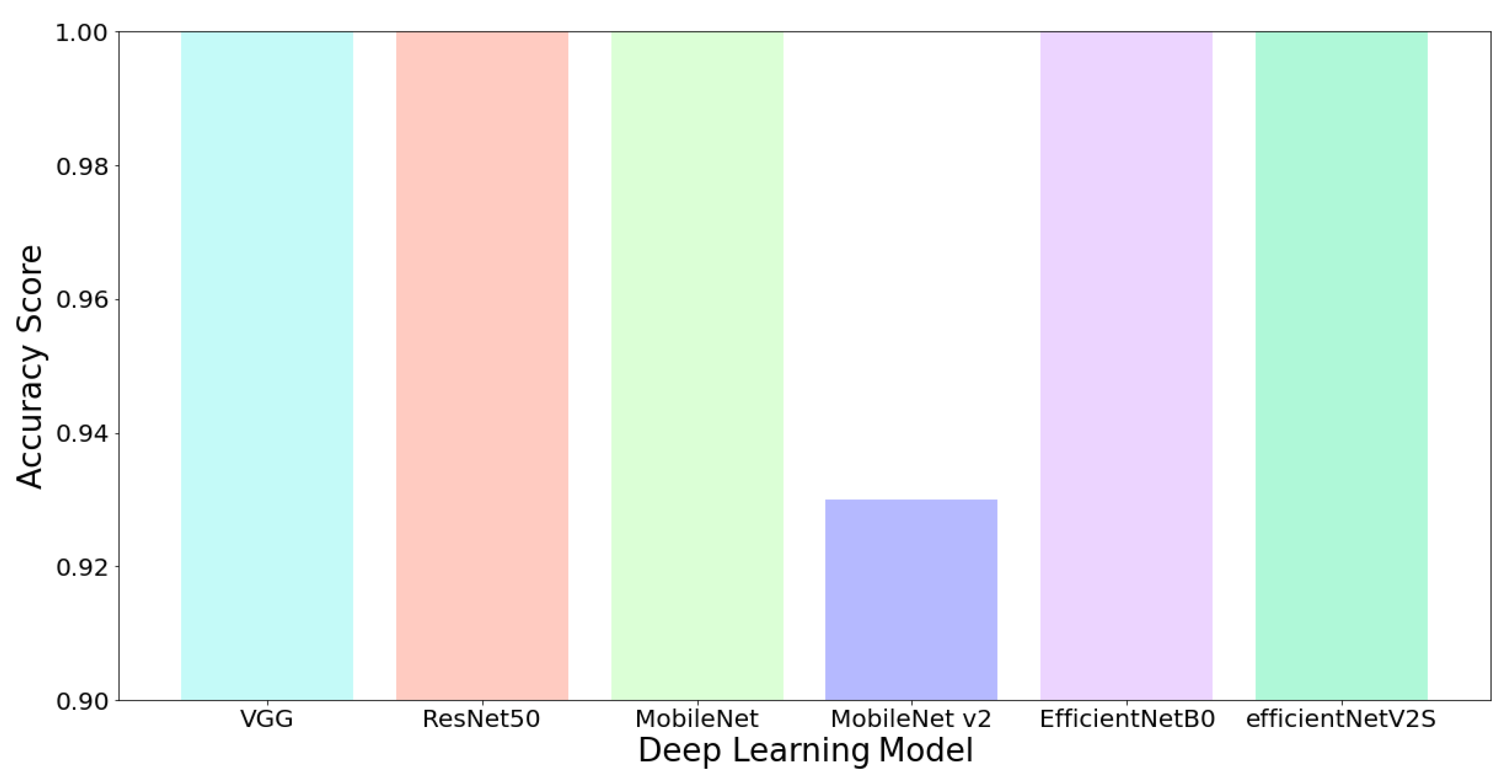
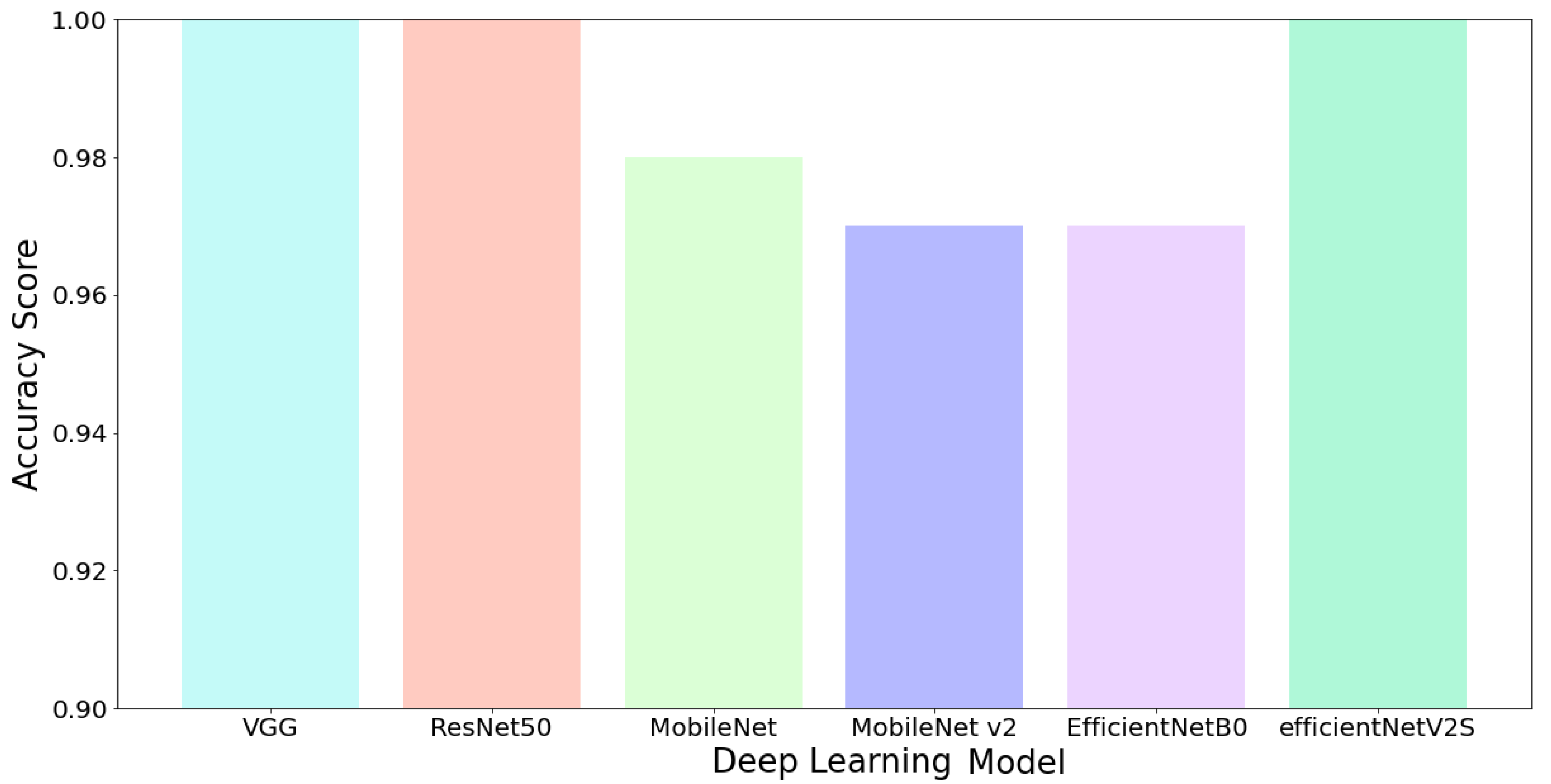
In this study, we trained six deep learning models to determine the quality of cylindrical shells. The model conducted the assessment process in real time, so a fast and accurate model was needed.
Figure 9 and
Figure 10 provide information on the accuracy gained from the entire model during the non-real-time testing process. Based on
Figure 9 and
Figure 10, it can be seen that deep learning models obtained excellent accuracy when tested with testing data. VGG and ResNet, the predecessors of the deep learning model, obtained very satisfactory results. In contrast, MobileNet v2, the lightest model, produced the lowest accuracy for both the longitudinal and the bottom sides. This low accuracy was due to the MobileNet v2 architecture having the lowest number of parameters in performing high-level feature extraction properly [
37].
Other issues must be considered when using deep learning in the real-world setting, namely the computational time and resources requirement. The computational time of a deep learning model can be seen through the number of parameters each model has [
38].
Table 1 provides information about the parameters of each model. Based on
Table 1, the model with the least number of parameters is MobileNet v2 and the one with the most is VGG.
The model selection used in the application is based on the resulting accuracy and the number of parameters. Of the overall models we use, the most recent model is EfficientNetV2. The model provides excellent accuracy, but in terms of the number of parameters, the model is not suitable for use because it has the third largest parameter. MobileNet v2 is claimed to be the lightest model, but this affects the accuracy produced. The resulting accuracy of MobileNet v2 is the lowest.
In this study, we selected the MobileNet v1 model because it did not differ significantly from MobileNet v2, and the number of parameters was between Mobilenet v2 and EfficientNet. In addition, MobileNet v1 also had equally good accuracy when assessing the quality of cylindrical shells. However, when conducting quality assessments on the longitudinal side, the accuracy was lower than that of VGG, ResNet, and EfficientNetV2S. Although VGG, ResNet, and EfficientNetV2S have stable accuracy, the number of parameters is a constraint when implementing in the real world.
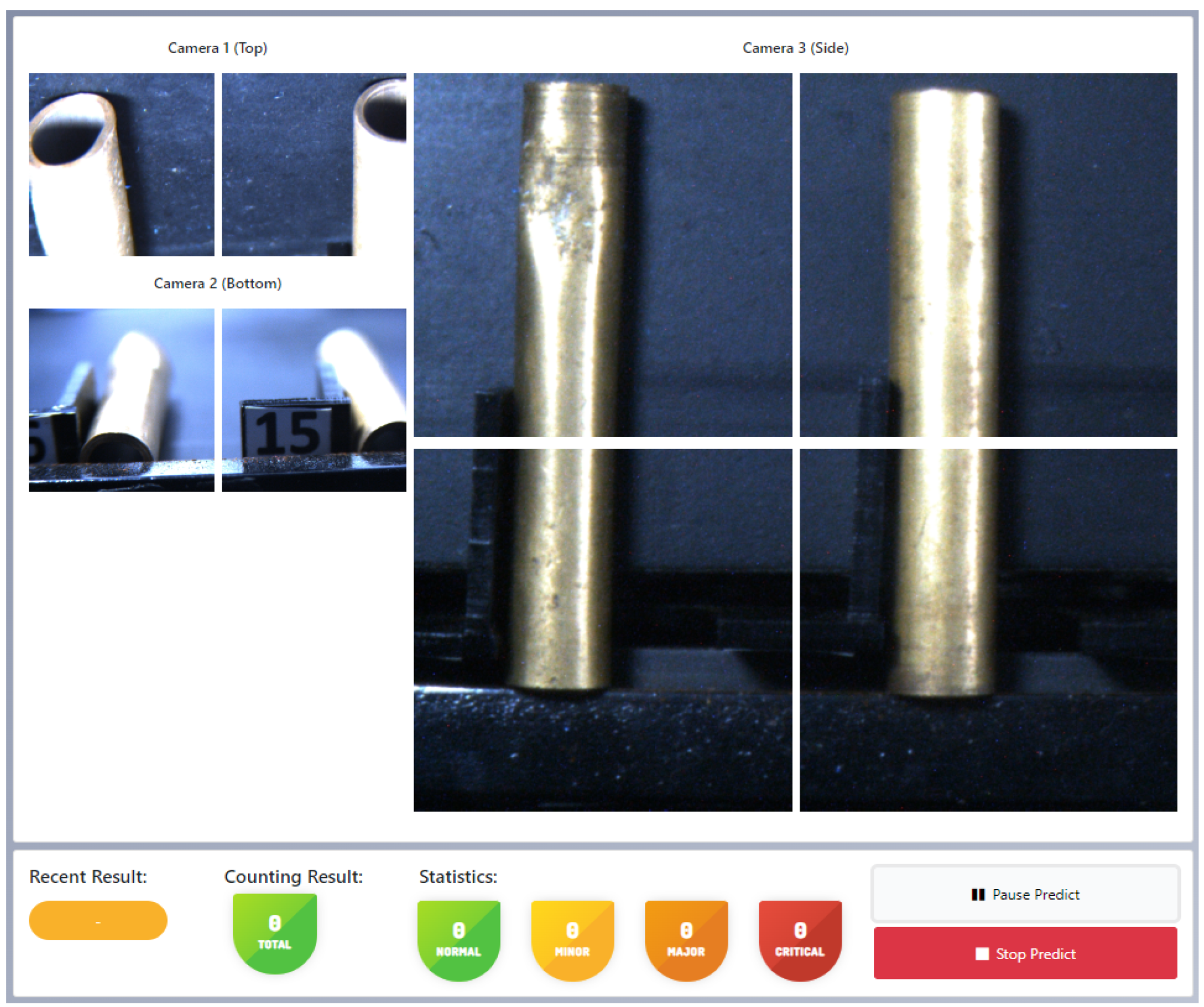
The web and desktop-based application user interface we built can be seen in
Figure 11. In
Figure 11, there are eight frames. The eight frames display the captured results from the high frame rate camera sensor. Each camera has two frames for the top and bottom sides, while the longitudinal side consists of four frames. The longitudinal side is divided into four frames because the captured object is a cylindrical shell object.
Each left and right side frame represents the part of the frame captured by the high frame rate camera sensor. Moreover, we split into two frames (for the top and bottom sides) and four frames specifically for the longitudinal side to optimize the image size processed by the deep learning model. This procedure was performed because the deep learning model used has been designed to accept inputs of the same size.
In this study, we focused on the web-based application because it is more straightforward to use. A web-based application is simpler because it can be created centrally. This feature is preferred because if there is a resource replacement, only the existing link needs to be accessed. The use of a web-based application can also be performed locally. In this study, we used a web-based application and placed a web server locally.
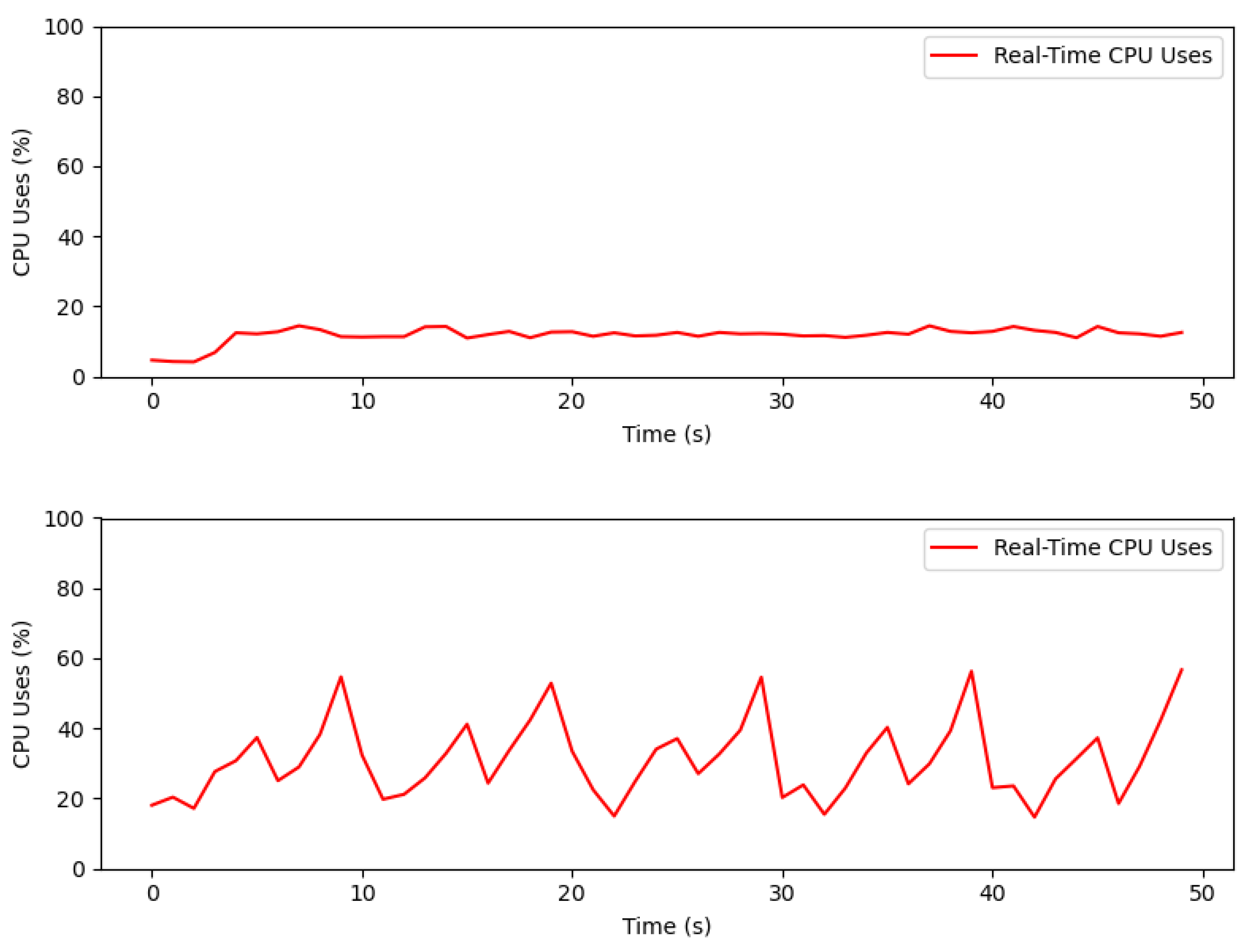
Before implementing the web-based application, we tried to develop a desktop-based application. Desktop-based development is more complex and inflexible. In order to use the desktop-based application, the application must first be installed, with a concomitant increase in CPU usage. In the desktop-based that we developed, when taking imagery through the high frame rate camera sensor, there was a very long delay, causing the assessment process to be sub-optimal and many frames to be missed. The image capture was only performed on one sensor camera. The delay became much longer when multiple sensor cameras were used. This longer delay occurred because the desktop-based application used the OpenCV library, which took time to capture imagery from the camera and convert it into an array format so that deep learning models could be used.
Figure 12 provides an overview of CPU usage in web-based and desktop-based applications.
Figure 12 shows that the use of a desktop-based CPU when using a high frame rate camera sensor already shows a graph with a reasonably high percentage. Unlike desktop-based, the web-based application provided much better results. This is because, in the web-based application, we used Javascripts that could directly capture images from the camera sensor and convert them into data types that deep learning models could process. The use of Javascripts certainly sped up the image retrieval process because it no longer used other libraries, as must be performed when developing a desktop-based application.
4. Conclusions
We propose optimizing computational resources for real-time product quality assessment on moving cylindrical shell objects using deep learning with multiple high frame rate camera sensors. The MobileNet v1 deep learning model was found to be the most suitable for real-time defect inspection compared to other deep learning models: VGG, ResNet, MobileNet v1, MobileNet v2, EfficientNet v1, and EfficientNet v2. The model is selected due to MobileNet v1 having a smaller number of parameters when compared to other deep learning models. More parameters will cause the training and testing process to be slow. The combination of interface and deep learning model is when MobileNet v1 is combined with a web-based application. The web-based application performs much better when compared to the desktop-based application. GPU and CPU resource usage when using the web-based application tended to be low, making the web-based application more suitable for most desktop computers. In addition, the web-based application can be placed centrally so that it is more flexible and can be accessed using a browser, so there is no need to carry out a complicated installation process.
Author Contributions
Conceptualization, A.W.; Methodology, A.W. and J.D.S.; Formal analysis, A.W.; Investigation, H.A. and A.A.S.M.M.J.M.; Resources, S.P.S., K.B.W., A.M., H.N. and B.K.; Writing—original draft, A.W. and J.D.S.; Writing—review & editing, J.D.S. and W.C.; Project administration, J.D.S.; Funding acquisition, J.D.S. and W.C. All authors have read and agreed to the published version of the manuscript.
Funding
This work was supported by the Kedaireka Grant—Indonesia, APBN Universitas Diponegoro Indonesia under Grant 132/UN7.A/KS/2022 with Joga Dharma Setiawan as PIC Investigator.
Data Availability Statement
Data is unavailable due to privacy or ethical restrictions.
Conflicts of Interest
The authors declare no conflict of interest.
References
- Ghorai, S.; Mukherjee, A.; Gangadaran, M.; Dutta, P.K. Automatic defect detection on hot-rolled flat steel products. IEEE Trans. Instrum. Meas. 2012, 62, 612–621. [Google Scholar] [CrossRef]
- Mohammad, S.M. Implementation Of Automation In Applications Of Healthcare, Private, And Public Sectors In IT. Int. J. Innov. Eng. Res. Technol. 2020, 7, 364–372. [Google Scholar]
- Sethu, M.; Titu, N.A.; Hu, D.; Madadi, M.; Coble, J.; Boring, R.; Blache, K.; Agarwal, V.; Yadav, V.; Khojandi, A. Using artificial intelligence to mitigate human factor errors in nuclear power plants: A review. Nuc Sci. Eng. 2021, 10, 1–13. [Google Scholar]
- Fang, X.; Luo, Q.; Zhou, B.; Li, C.; Tian, L. Research progress of automated visual surface defect detection for industrial metal planar materials. Sensors 2020, 20, 5136. [Google Scholar] [CrossRef] [PubMed]
- Parekh, D.; Poddar, N.; Rajpurkar, A.; Chahal, M.; Kumar, N.; Joshi, G.P.; Cho, W. A Review on Autonomous Vehicles: Progress, Methods and Challenges. Electronics 2022, 11, 2162. [Google Scholar] [CrossRef]
- Collins, C.; Dennehy, D.; Conboy, K.; Mikalef, P. Artificial intelligence in information systems research: A systematic literature review and research agenda. Int. J. Inf. Manag. 2021, 60, 102383. [Google Scholar] [CrossRef]
- Chaudhuri, S.; Krishnan Lrk, P.S. Impact of Using AI in Manufacturing Industries. J. Int. Acad. Case Stud. 2022, 28. [Google Scholar]
- Tao, X.; Zhang, D.; Ma, W.; Liu, X.; Xu, D. Automatic metallic surface defect detection and recognition with convolutional neural networks. Appl. Sci. 2018, 8, 1575. [Google Scholar] [CrossRef]
- Zhang, Y.; You, D.; Gao, X.; Zhang, N.; Gao, P.P. Welding defects detection based on deep learning with multiple optical sensors during disk laser welding of thick plates. J. Manuf. Syst. 2019, 51, 87–94. [Google Scholar] [CrossRef]
- Singh, S.A.; Desai, K. Automated surface defect detection framework using machine vision and convolutional neural networks. J. Intell. Manuf. 2022, 1–17. [Google Scholar] [CrossRef]
- Wang, J.; Fu, P.; Gao, R.X. Machine vision intelligence for product defect inspection based on deep learning and Hough transform. J. Manuf. Syst. 2019, 51, 52–60. [Google Scholar] [CrossRef]
- Anthony, A.; Ho, E.S.; Woo, W.L.; Gao, B. A Review and Benchmark on State-of-the-Art Steel Defects Detection. Available online: https://papers.ssrn.com/sol3/papers.cfm?abstract_id=4121951 (accessed on 20 January 2023).
- Tao, J.; Zhu, Y.; Jiang, F.; Liu, H.; Liu, H. Rolling Surface Defect Inspection for Drum-Shaped Rollers Based on Deep Learning. IEEE Sens. J. 2022, 22, 8693–8700. [Google Scholar] [CrossRef]
- Xie, R.; Zhu, Y.; Luo, J.; QIn, G.; Wang, D. Detection Algorithm of Bearing Roller End Surface Defects Based on Improved YOLOv5n and Image Fusion. Meas. Sci. Technol. 2023, 34, 045402. [Google Scholar] [CrossRef]
- Fu, G.; Sun, P.; Zhu, W.; Yang, J.; Cao, Y.; Yang, M.Y.; Cao, Y. A deep-learning-based approach for fast and robust steel surface defects classification. Opt. Lasers Eng. 2019, 121, 397–405. [Google Scholar] [CrossRef]
- Khan, M.F.; Alam, A.; Siddiqui, M.A.; Alam, M.S.; Rafat, Y.; Salik, N.; Al-Saidan, I. Real-time defect detection in 3D printing using machine learning. Mater. Today Proc. 2021, 42, 521–528. [Google Scholar] [CrossRef]
- Kang, G.; Gao, S.; Yu, L.; Zhang, D. Deep architecture for high-speed railway insulator surface defect detection: Denoising autoencoder with multitask learning. IEEE Trans. Instrum. Meas. 2018, 68, 2679–2690. [Google Scholar] [CrossRef]
- Zhang, J.; Huang, D.; Hu, T.; Fuchikami, R.; Ikenaga, T. Critically Compressed Quantized Convolution Neural Network based High Frame Rate and Ultra-Low Delay Fruit External Defects Detection. In Proceedings of the 2021 17th International Conference on Machine Vision and Applications (MVA), Aichi, Japan, 25–27 July 2021; pp. 1–4. [Google Scholar]
- Albanese, A.; Nardello, M.; Fiacco, G.; Brunelli, D. Tiny Machine Learning for High Accuracy Product Quality Inspection. IEEE Sens. J. 2022, 23, 1575–1583. [Google Scholar] [CrossRef]
- Kiani Galoogahi, H.; Fagg, A.; Huang, C.; Ramanan, D.; Lucey, S. Need for speed: A benchmark for higher frame rate object tracking. In Proceedings of the IEEE International Conference on Computer Vision, Venice, Italy, 22–29 October 2017; pp. 1125–1134. [Google Scholar]
- Krizhevsky, A.; Sutskever, I.; Hinton, G.E. Imagenet classification with deep convolutional neural networks. Commun. ACM 2017, 60, 84–90. [Google Scholar] [CrossRef]
- Simonyan, K.; Zisserman, A. Very deep convolutional networks for large-scale image recognition. arXiv 2014, arXiv:1409.1556. [Google Scholar]
- He, K.; Zhang, X.; Ren, S.; Sun, J. Deep residual learning for image recognition. In Proceedings of the IEEE Conference on Computer Vision and Pattern Recognition, Las Vegas, NV, USA, 27–30 June 2016; pp. 770–778. [Google Scholar]
- Saini, S.S.; Rawat, P. Deep Residual Network for Image Recognition. In Proceedings of the 2022 IEEE International Conference on Distributed Computing and Electrical Circuits and Electronics (ICDCECE), Ballari, India, 23–24 April 2022; pp. 1–4. [Google Scholar]
- Sun, L.; Resnet on Tiny Imagenet. Submitted on 14 February 2016. 2016. Available online: http://vision.stanford.edu/teaching/cs231n/reports/2017/pdfs/12.pdf (accessed on 30 December 2022).
- Howard, A.G.; Zhu, M.; Chen, B.; Kalenichenko, D.; Wang, W.; Weyand, T.; Andreetto, M.; Adam, H. Mobilenets: Efficient convolutional neural networks for mobile vision applications. arXiv 2017, arXiv:1704.04861. [Google Scholar]
- Sandler, M.; Howard, A.; Zhu, M.; Zhmoginov, A.; Chen, L.C. Mobilenetv2: Inverted residuals and linear bottlenecks. In Proceedings of the IEEE Conference on Computer Vision and Pattern Recognition, Salt Lake City, UT, USA, 18–22 June 2018; pp. 4510–4520. [Google Scholar]
- Tan, M.; Le, Q. Efficientnet: Rethinking model scaling for convolutional neural networks. In Proceedings of the International Conference on Machine Learning. PMLR, Long Beach, CA, USA, 9–15 June 2019; pp. 6105–6114. [Google Scholar]
- Tan, M.; Le, Q. Efficientnetv2: Smaller models and faster training. In Proceedings of the International Conference on Machine Learning. PMLR, Virtual Event, 18–24 July 2021; pp. 10096–10106. [Google Scholar]
- Gupta, S.; Tan, M. EfficientNet-EdgeTPU: Creating accelerator-optimized neural networks with AutoML. Google AI Blog 2019, 2, 1. [Google Scholar]
- Rampasek, L.; Goldenberg, A. TensorFlow: Biology’s gateway to deep learning? Cell Syst. 2016, 2, 12–14. [Google Scholar] [CrossRef] [PubMed]
- Culjak, I.; Abram, D.; Pribanic, T.; Dzapo, H.; Cifrek, M. A brief introduction to OpenCV. In Proceedings of the 2012 35th International Convention MIPRO, Opatija, Croatia, 21–25 May 2012; pp. 1725–1730. [Google Scholar]
- Ruder, S. An overview of gradient descent optimization algorithms. arXiv 2016, arXiv:1609.04747. [Google Scholar]
- Géron, A. Hands-on Machine Learning with Scikit-Learn, Keras, and TensorFlow; O’Reilly Media, Inc.: Sebastopol, CA, USA, 2022. [Google Scholar]
- Kingma, D.P.; Ba, J. Adam: A method for stochastic optimization. arXiv 2014, arXiv:1412.6980. [Google Scholar]
- Blagec, K.; Dorffner, G.; Moradi, M.; Samwald, M. A critical analysis of metrics used for measuring progress in artificial intelligence. arXiv 2020, arXiv:2008.02577. [Google Scholar]
- Shahi, T.B.; Sitaula, C.; Neupane, A.; Guo, W. Fruit classification using attention-based MobileNetV2 for industrial applications. PLoS ONE 2022, 17, e0264586. [Google Scholar] [CrossRef]
- Denil, M.; Shakibi, B.; Dinh, L.; Ranzato, M.; De Freitas, N. Predicting parameters in deep learning. Adv. Neural Inf. Process. Syst. 2013, 26. [Google Scholar]
| Disclaimer/Publisher’s Note: The statements, opinions and data contained in all publications are solely those of the individual author(s) and contributor(s) and not of MDPI and/or the editor(s). MDPI and/or the editor(s) disclaim responsibility for any injury to people or property resulting from any ideas, methods, instructions or products referred to in the content. |
© 2023 by the authors. Licensee MDPI, Basel, Switzerland. This article is an open access article distributed under the terms and conditions of the Creative Commons Attribution (CC BY) license (https://creativecommons.org/licenses/by/4.0/).


 ,
, 


