Author Contributions
Conceptualization, N.S. and R.S.; methodology, R.S. and P.S.; software, P.S.; validation, R.S. and P.S.; formal analysis, R.S.; investigation, N.S., R.S. and P.S.; writing—original draft preparation, R.S.; writing—review and editing, R.S., P.S. and N.S.; visualization, R.S., P.S. and N.S. All authors have read and agreed to the published version of the manuscript.
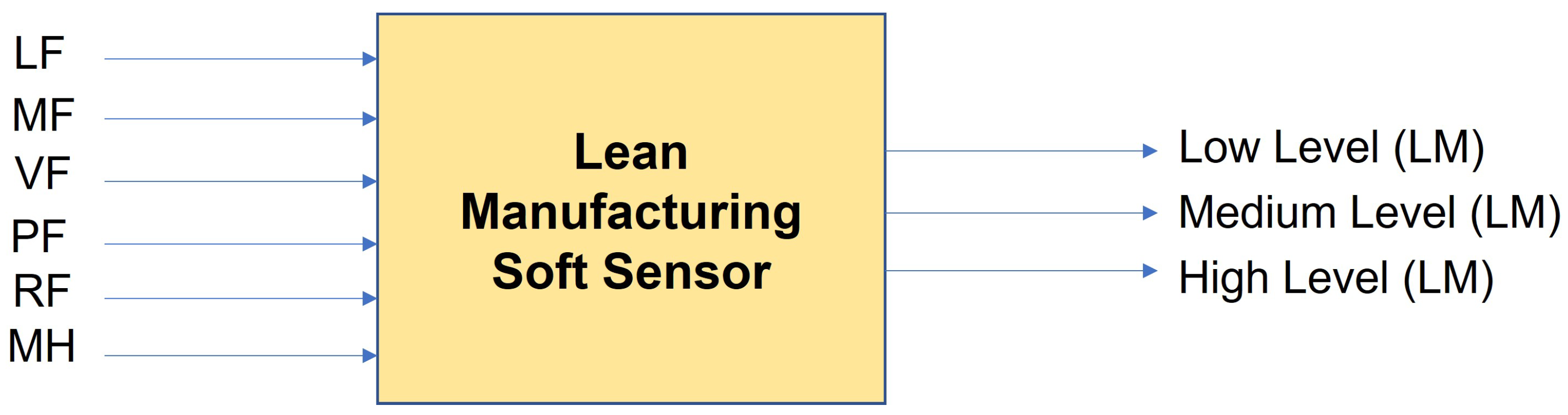
Figure 1.
Block Diagram of LM Soft Sensor.
Figure 1.
Block Diagram of LM Soft Sensor.
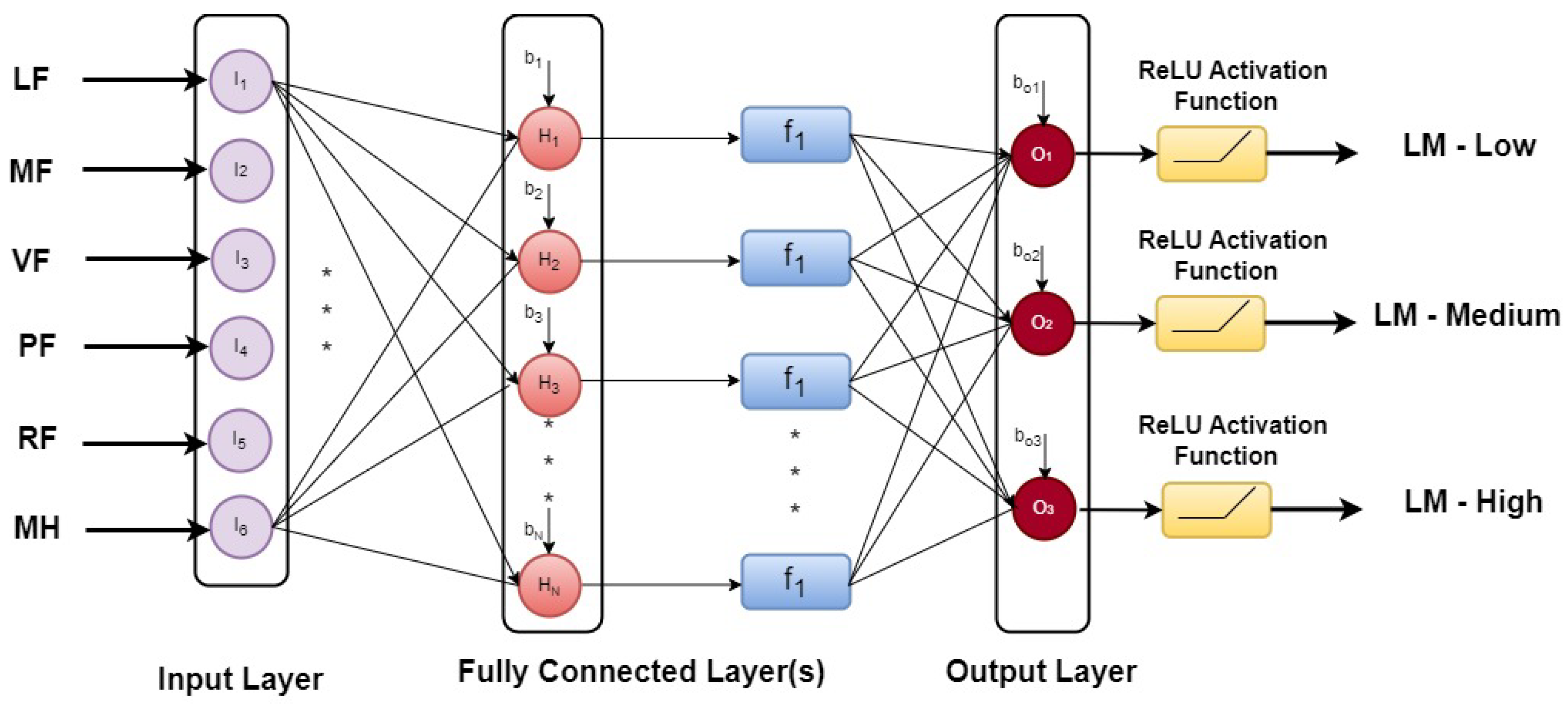
Figure 2.
ANN Classification. ‘∗’ indicates the presence of multiple instances of the same feature.
Figure 2.
ANN Classification. ‘∗’ indicates the presence of multiple instances of the same feature.
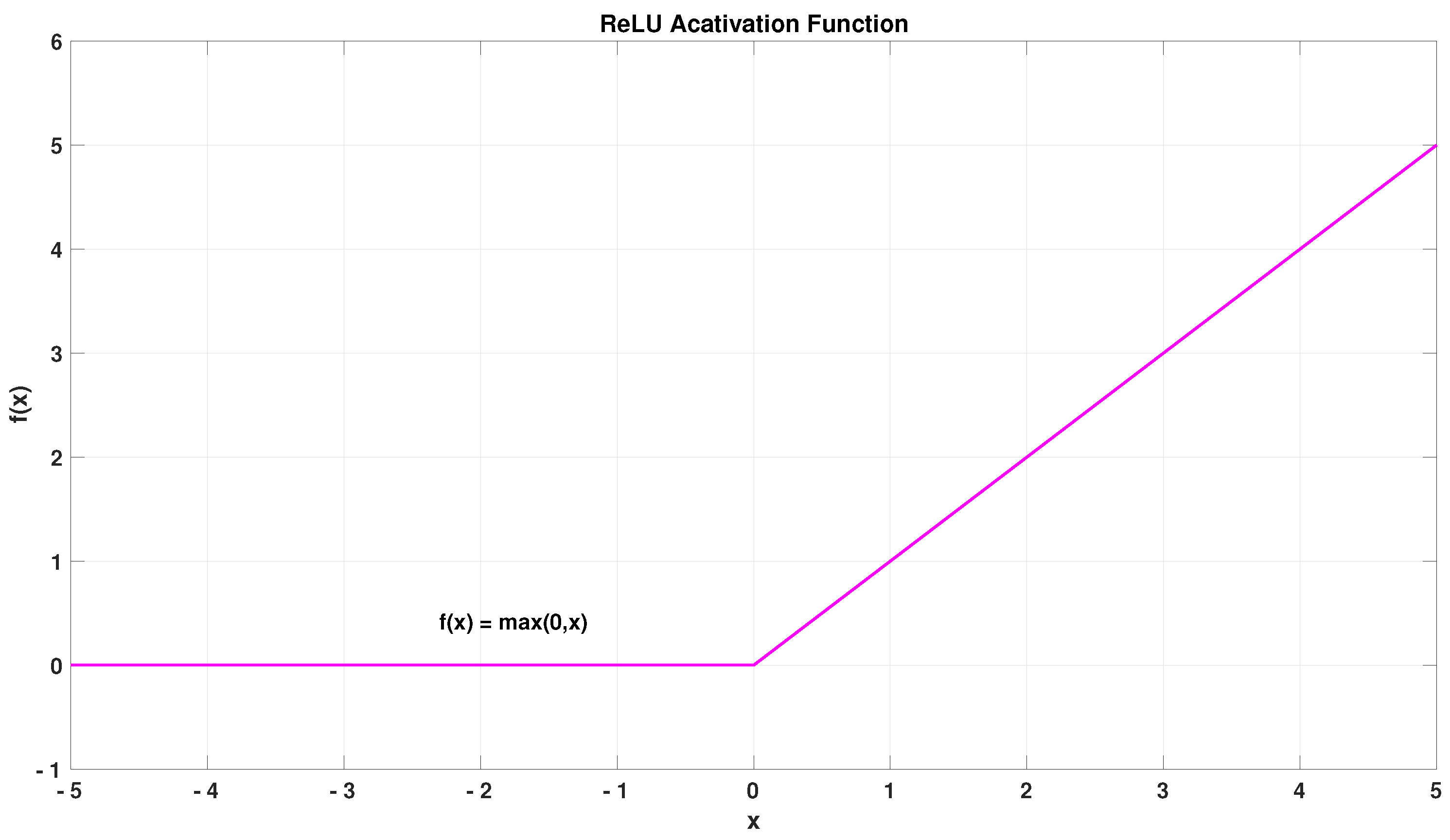
Figure 3.
ReLU Activation Function.
Figure 3.
ReLU Activation Function.
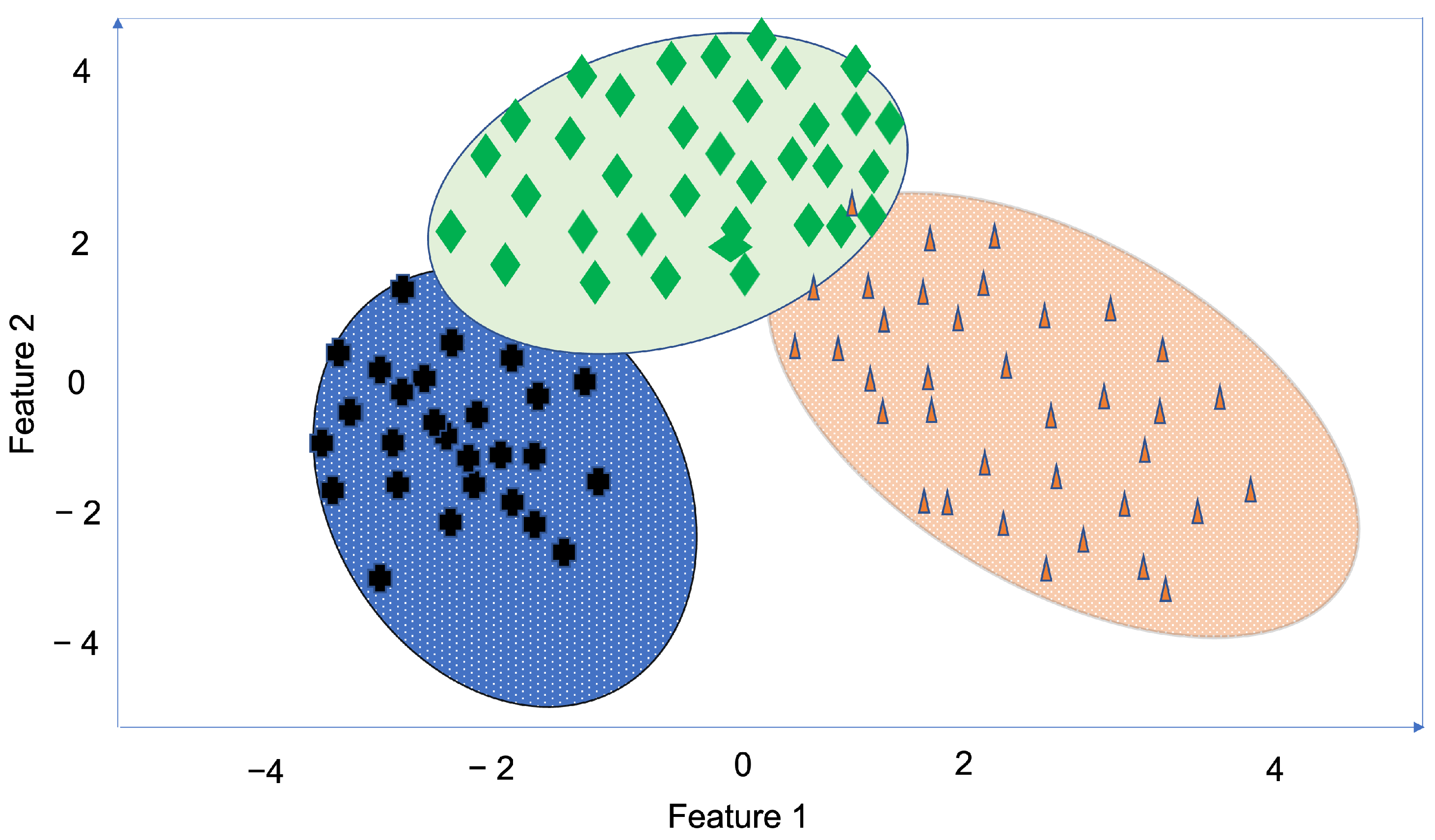
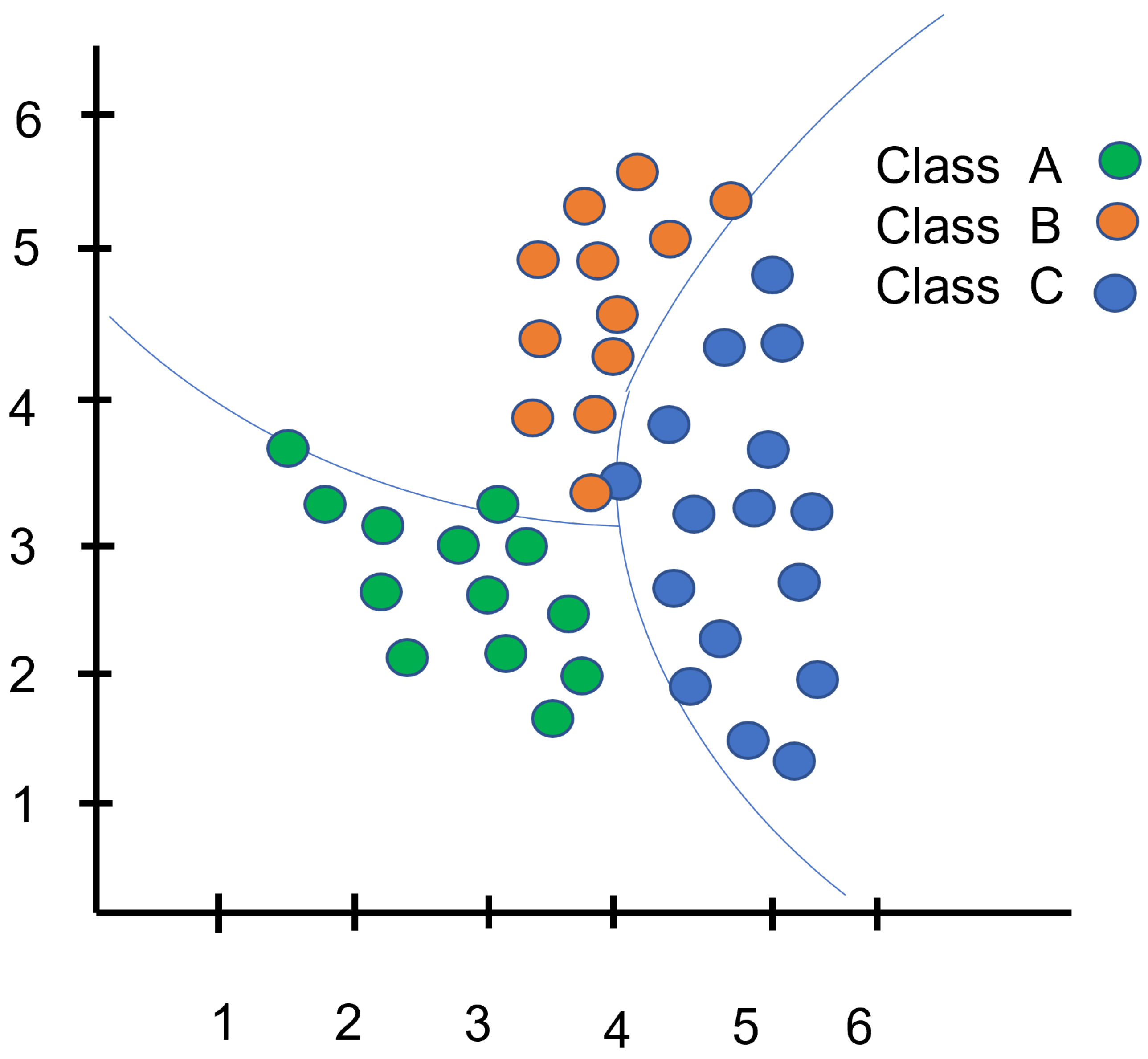
Figure 4.
KNN Classification.
Figure 4.
KNN Classification.
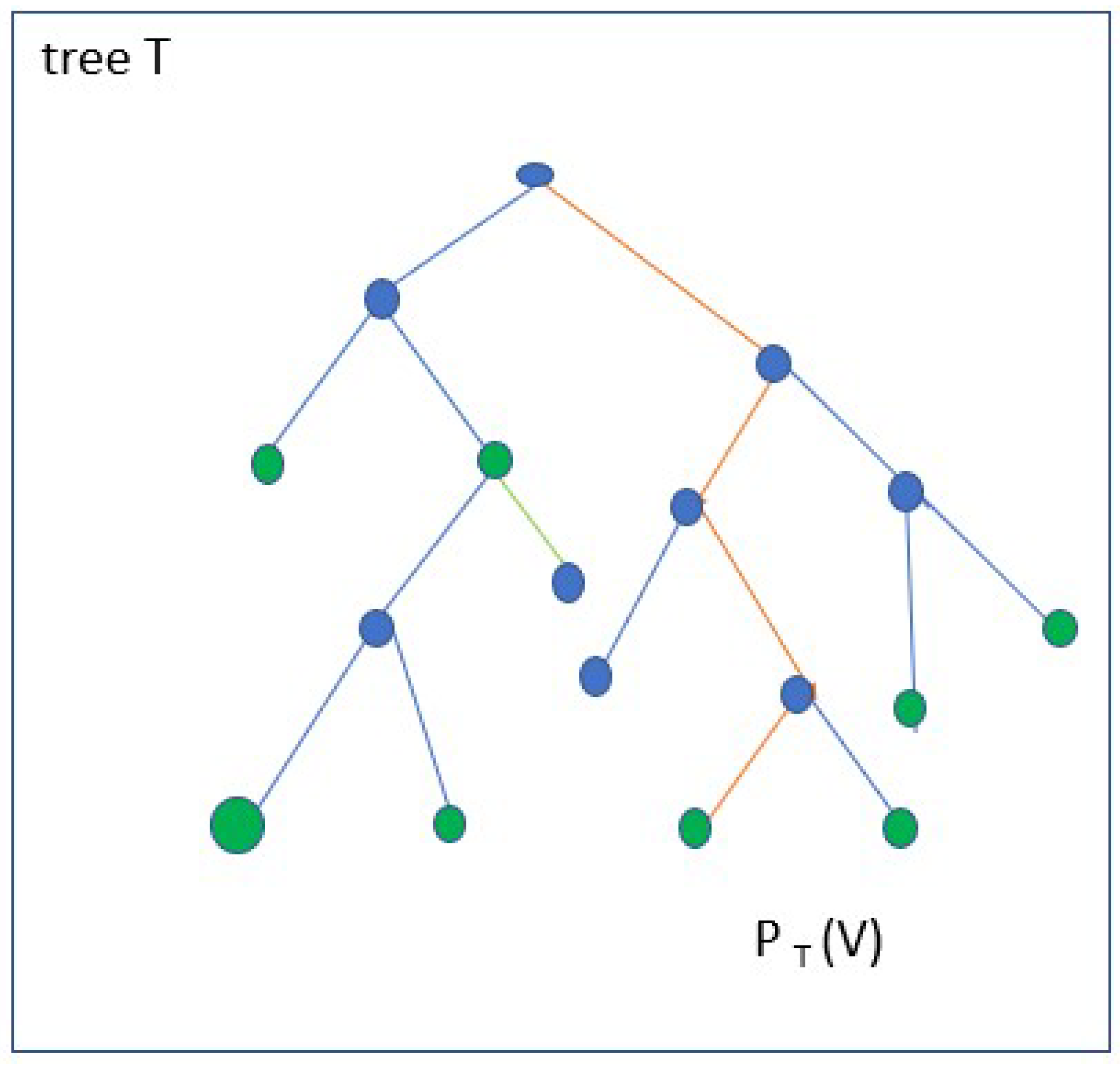
Figure 5.
Tree Classification.
Figure 5.
Tree Classification.
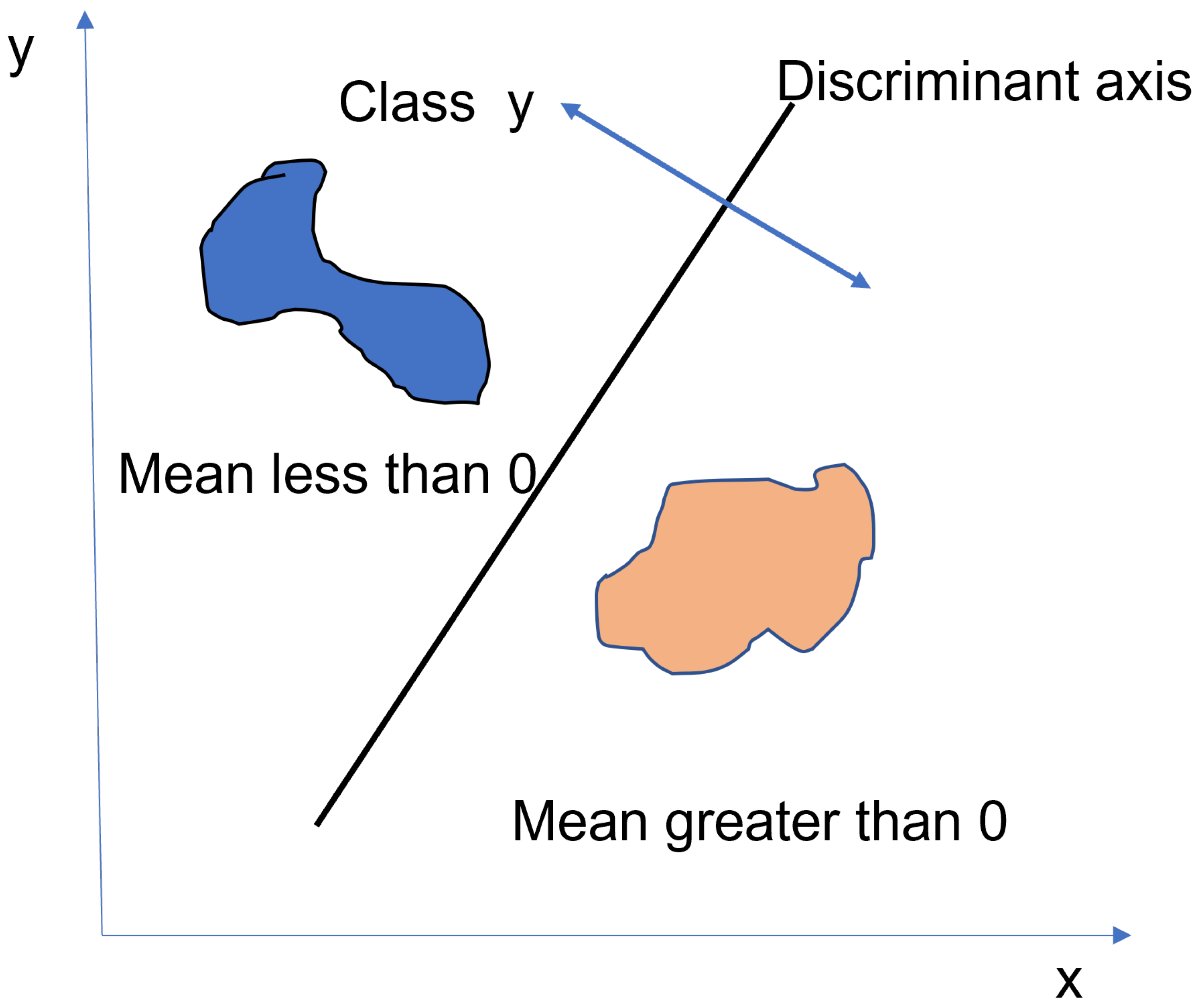
Figure 6.
Discriminant Classification.
Figure 6.
Discriminant Classification.
Figure 7.
Naive Bayes Classification.
Figure 7.
Naive Bayes Classification.
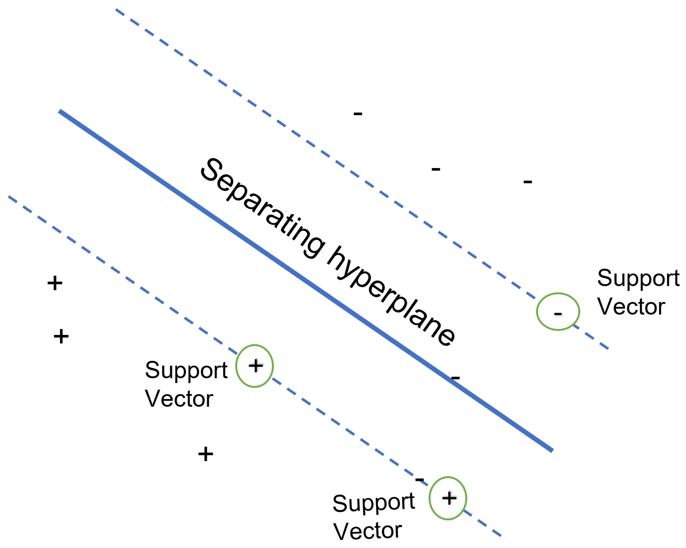
Figure 8.
SVM Classification.
Figure 8.
SVM Classification.
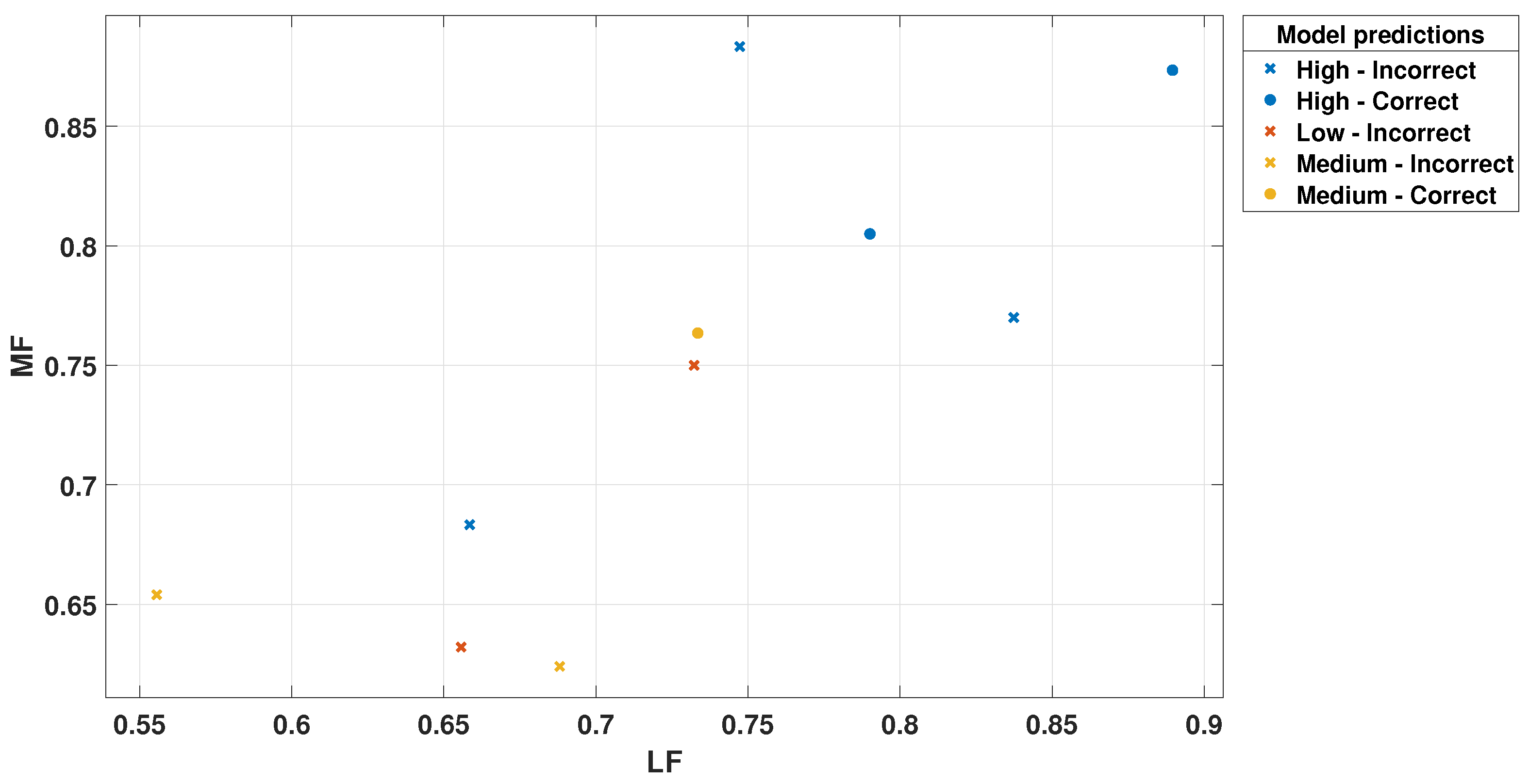
Figure 9.
LF Scatter Plot for Trilayered Neural Network.
Figure 9.
LF Scatter Plot for Trilayered Neural Network.
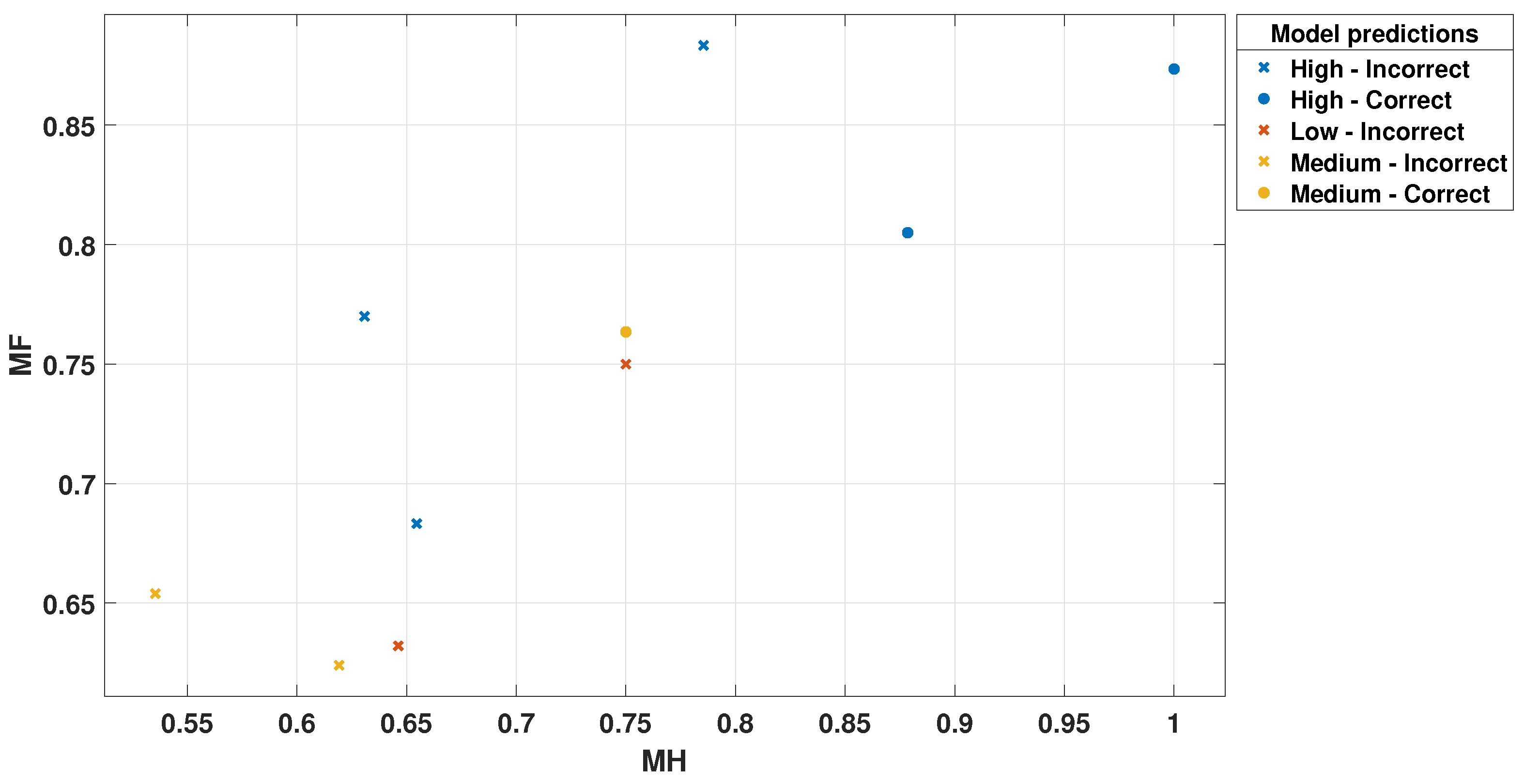
Figure 10.
MH Scatter Plot for Trilayered Neural Network.
Figure 10.
MH Scatter Plot for Trilayered Neural Network.
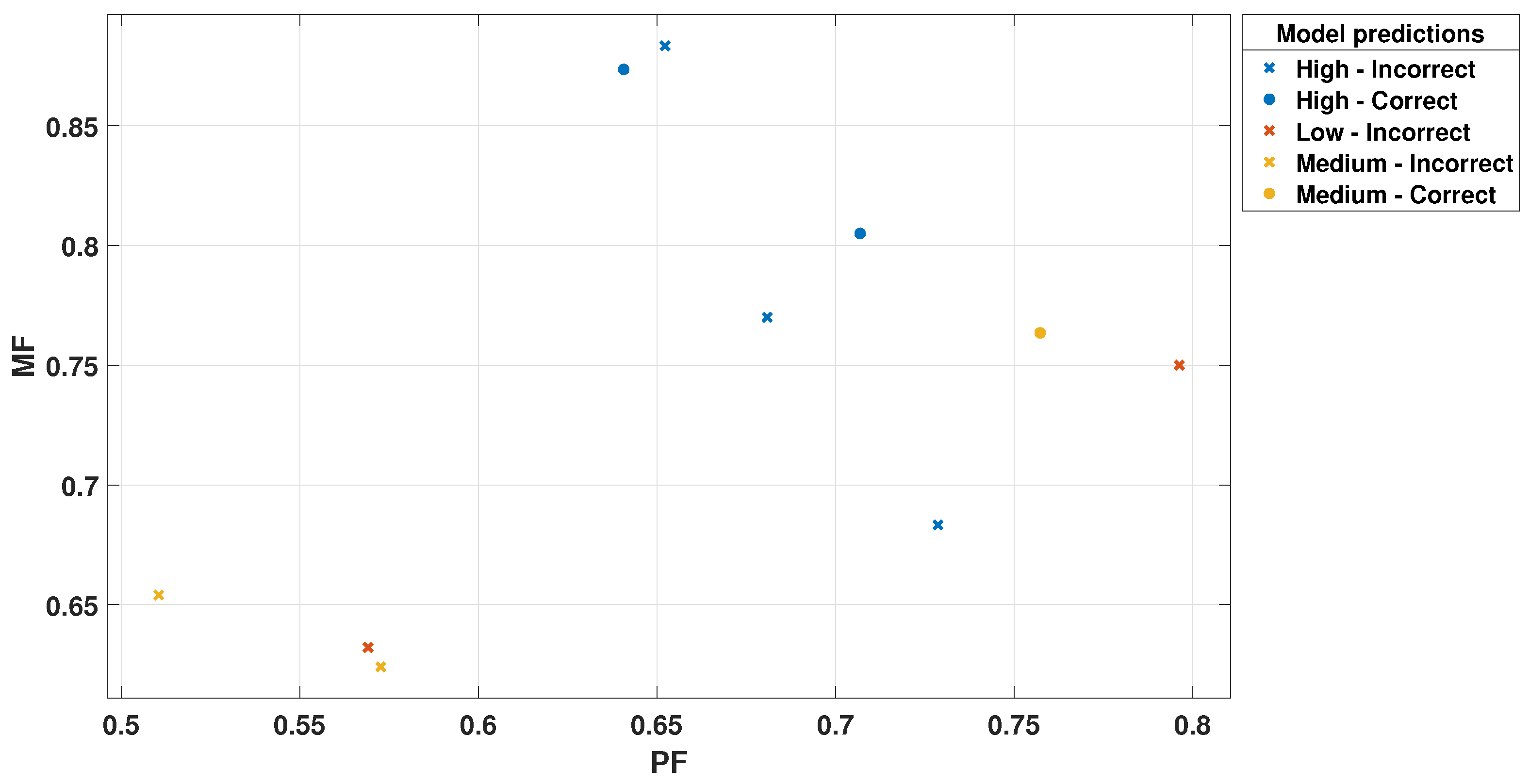
Figure 11.
PF Scatter Plot for Trilayered Neural Network.
Figure 11.
PF Scatter Plot for Trilayered Neural Network.
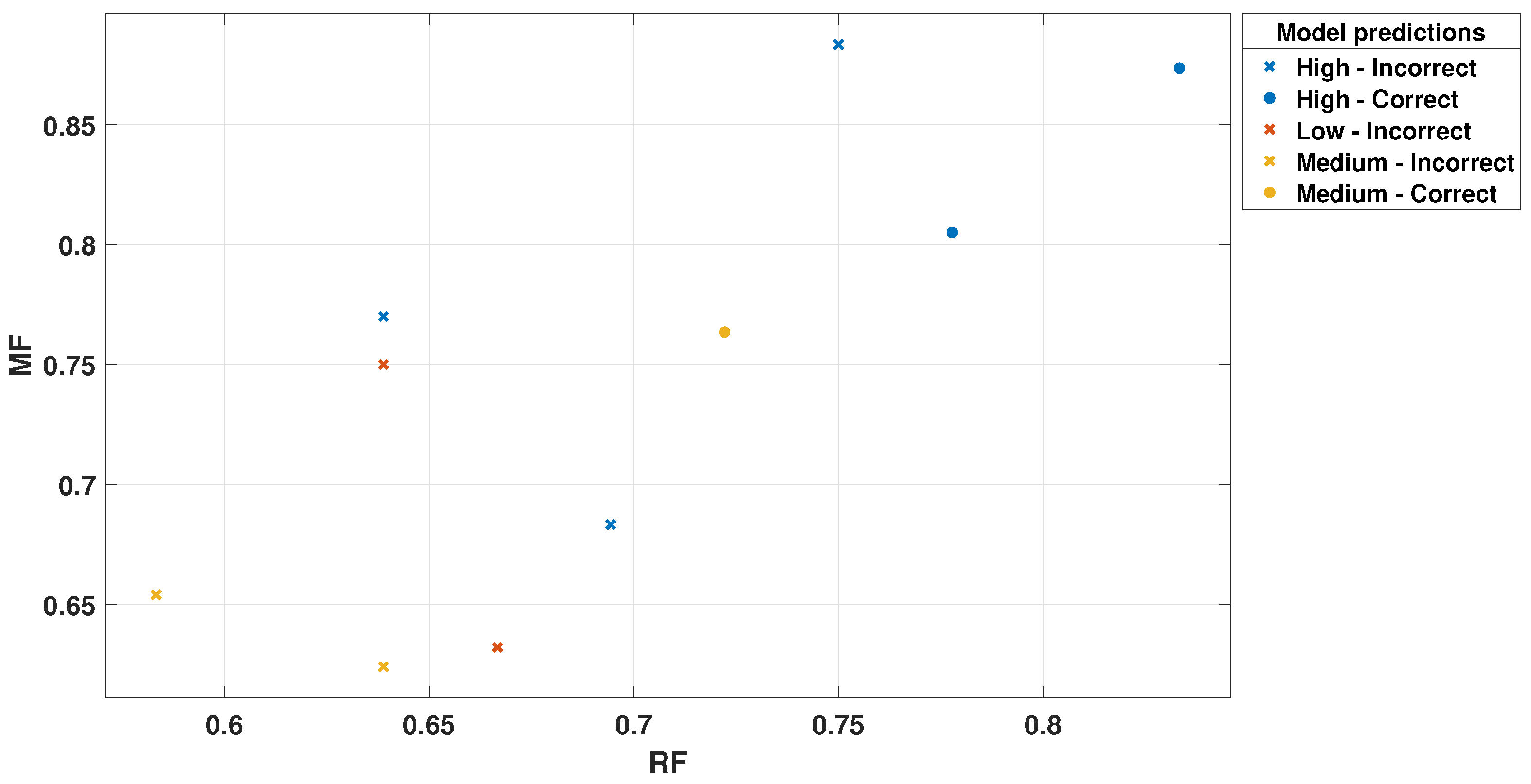
Figure 12.
RF Scatter Plot for Trilayered Neural Network.
Figure 12.
RF Scatter Plot for Trilayered Neural Network.
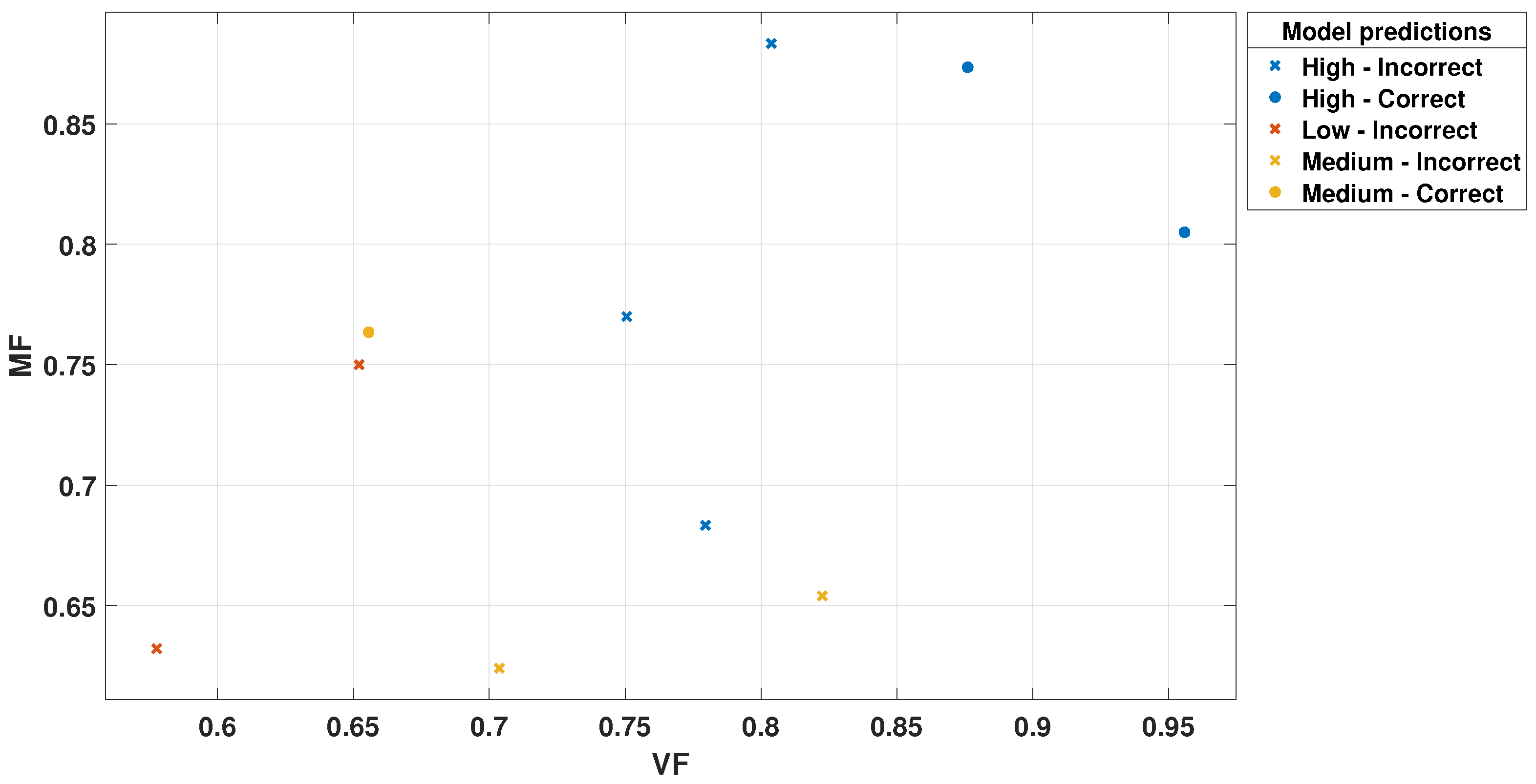
Figure 13.
VF Scatter Plot for Trilayered Neural Network.
Figure 13.
VF Scatter Plot for Trilayered Neural Network.
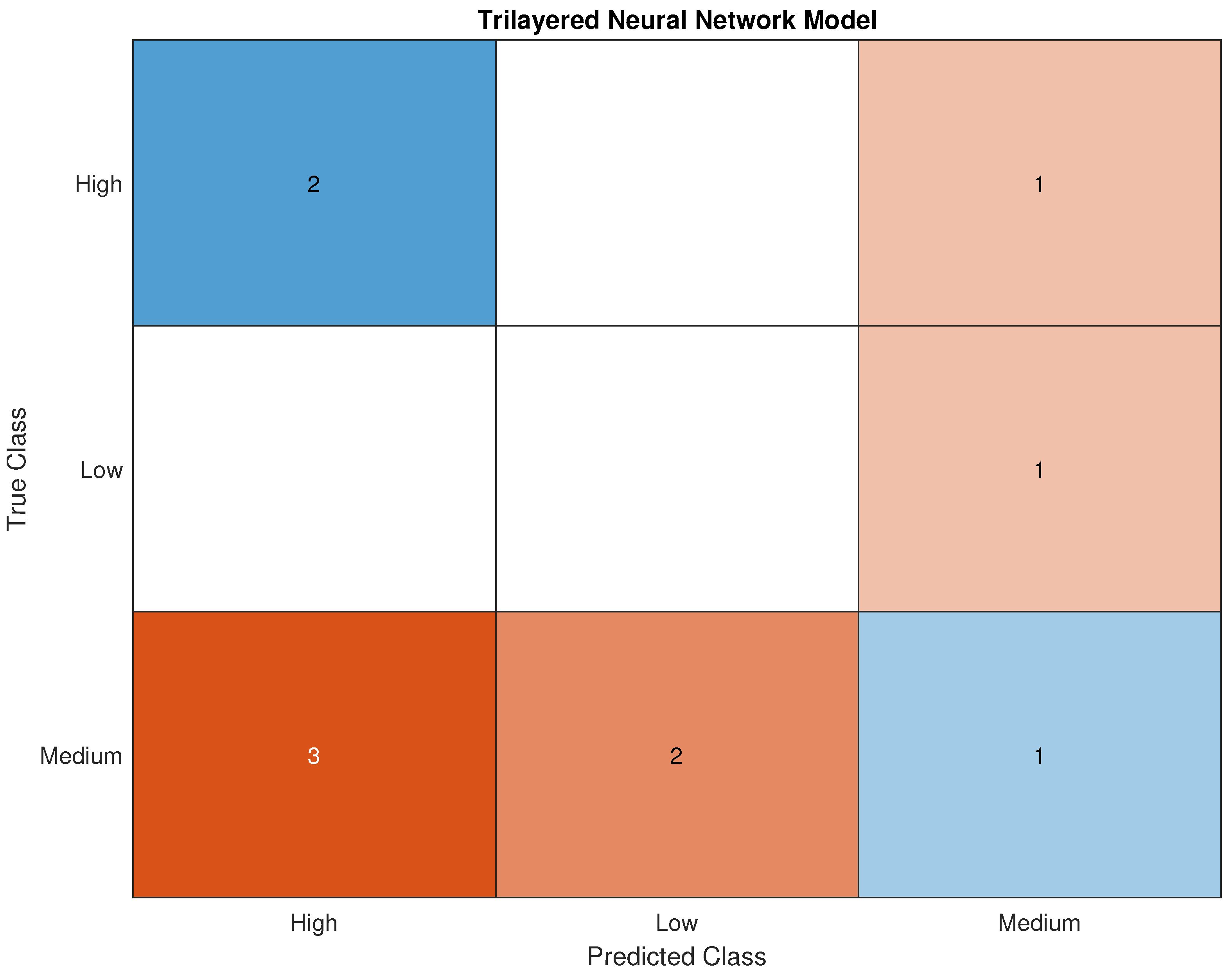
Figure 14.
Validation Confusion Matrix for Trilayered Neural Network.
Figure 14.
Validation Confusion Matrix for Trilayered Neural Network.
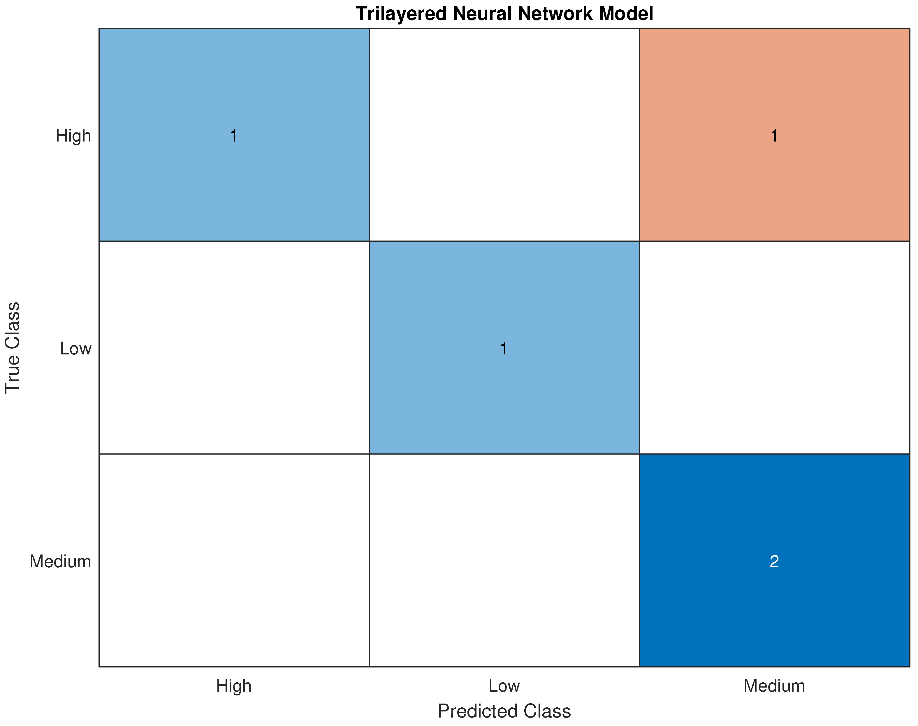
Figure 15.
Testing Confusion Matrix for Trilayered Neural Network.
Figure 15.
Testing Confusion Matrix for Trilayered Neural Network.
Figure 16.
Validation ROC for Trilayered Neural Network for High Class.
Figure 16.
Validation ROC for Trilayered Neural Network for High Class.
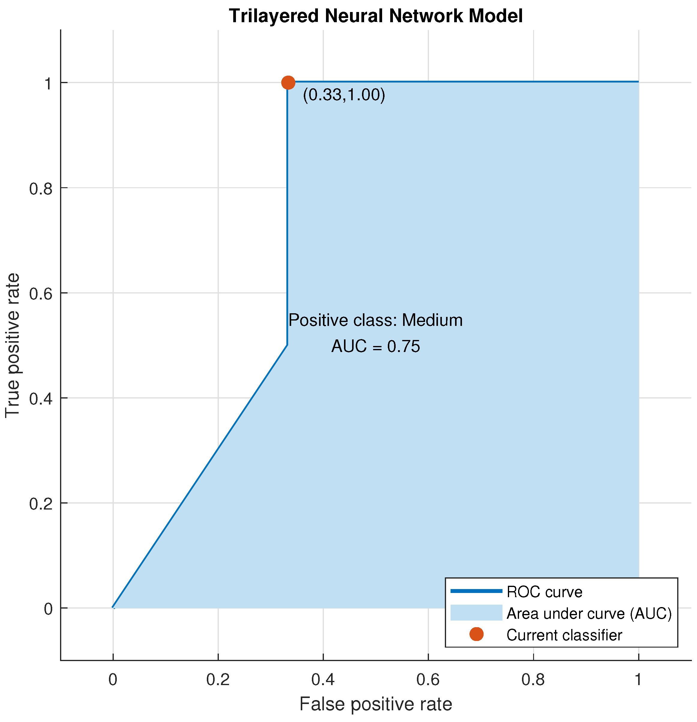
Figure 17.
Validation ROC for Trilayered Neural Network for Medium Class.
Figure 17.
Validation ROC for Trilayered Neural Network for Medium Class.
Figure 18.
Validation ROC for Trilayered Neural Network for Low Class.
Figure 18.
Validation ROC for Trilayered Neural Network for Low Class.
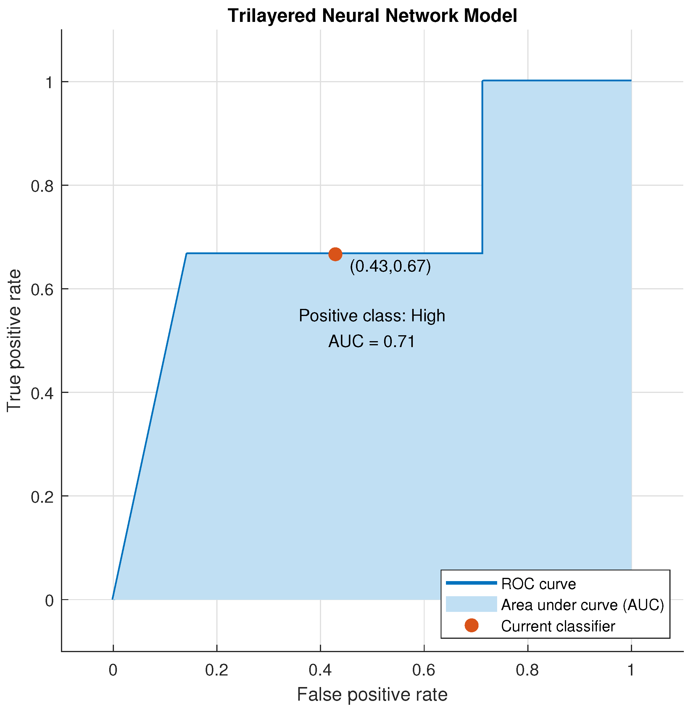
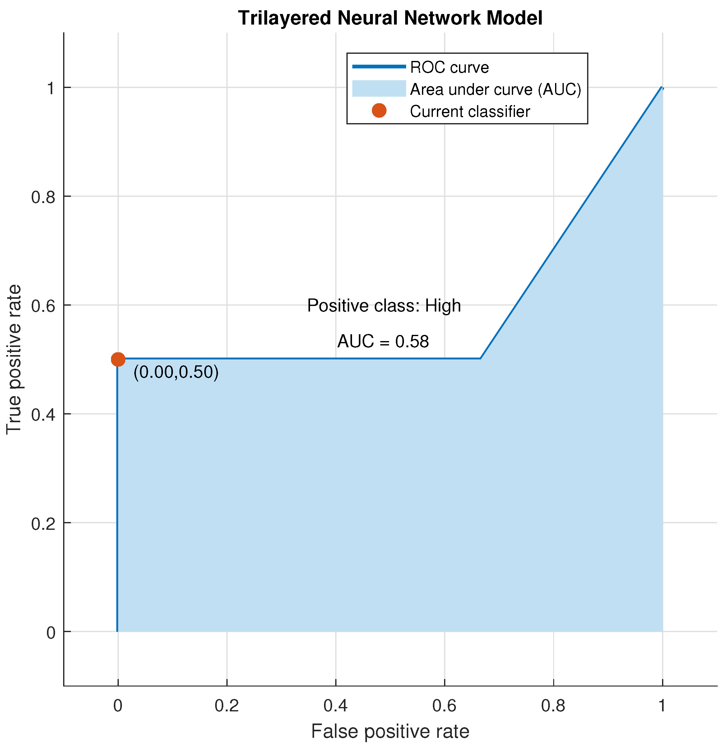
Figure 19.
Testing ROC for Trilayered Neural Network for High Class.
Figure 19.
Testing ROC for Trilayered Neural Network for High Class.
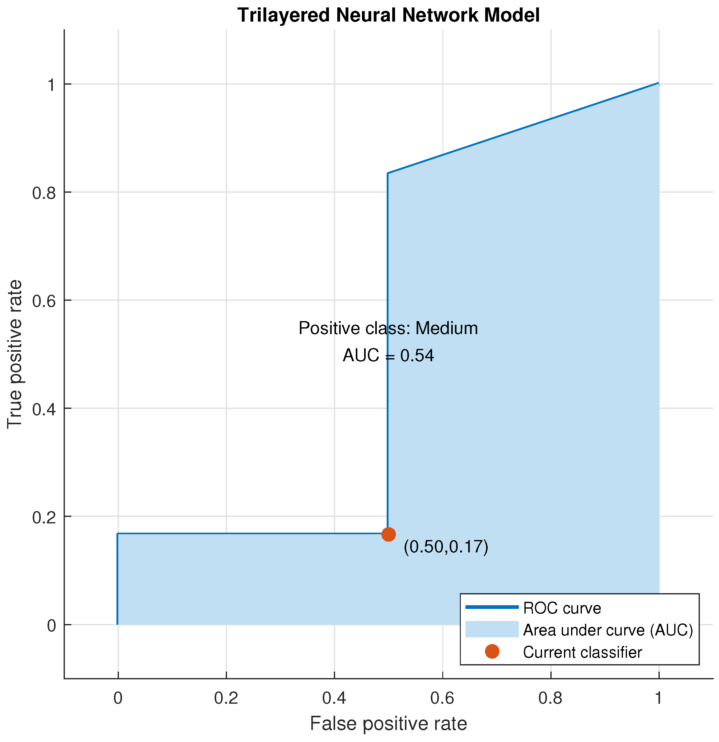
Figure 20.
Testing ROC for Trilayered Neural Network for Medium Class.
Figure 20.
Testing ROC for Trilayered Neural Network for Medium Class.
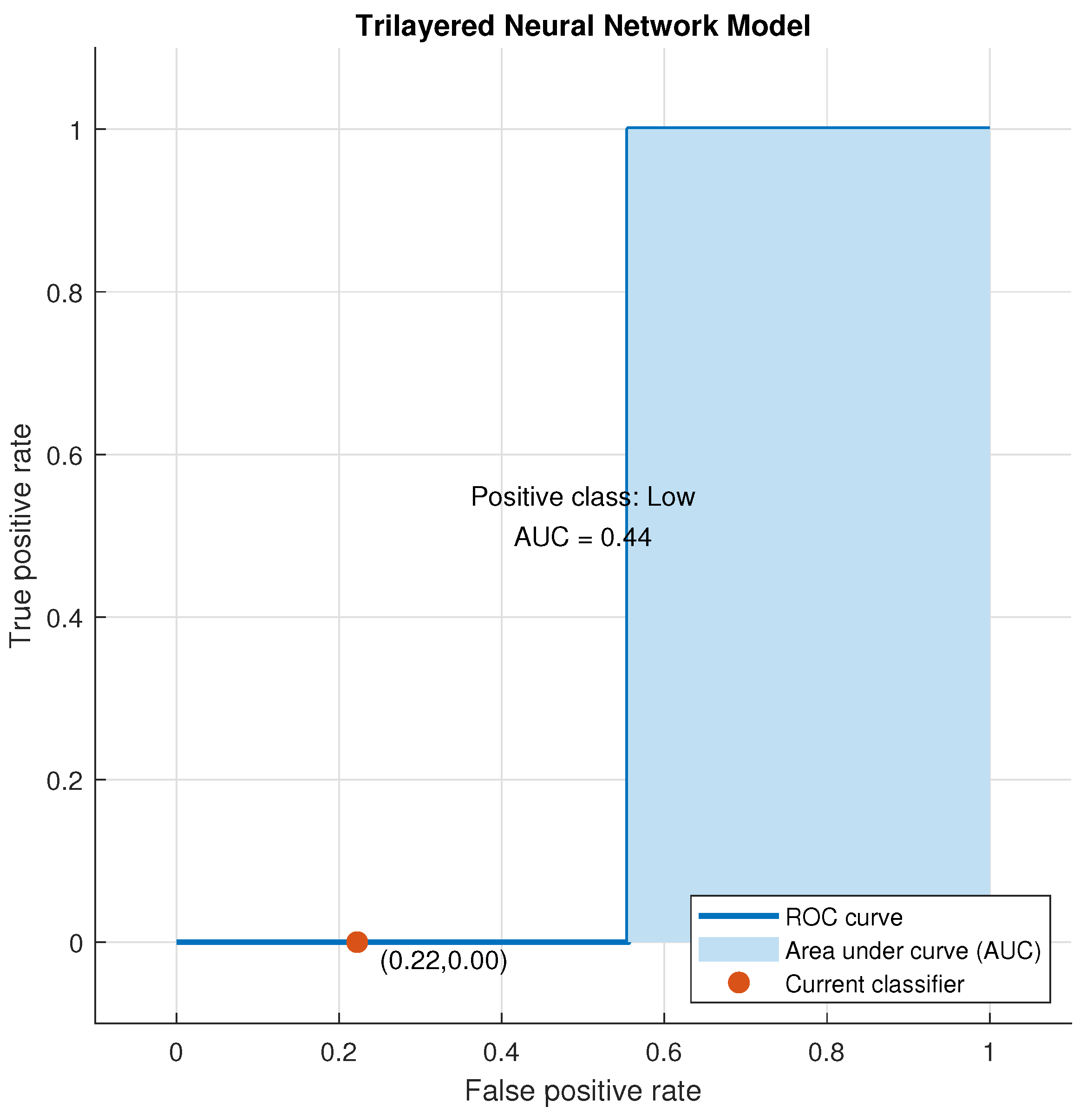
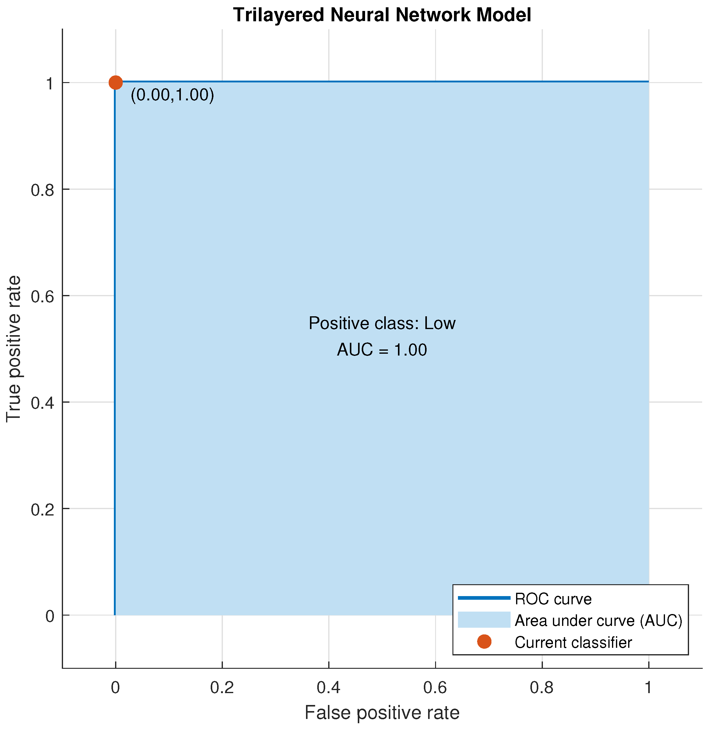
Figure 21.
Testing ROC for Trilayered Neural Network for Low Class.
Figure 21.
Testing ROC for Trilayered Neural Network for Low Class.
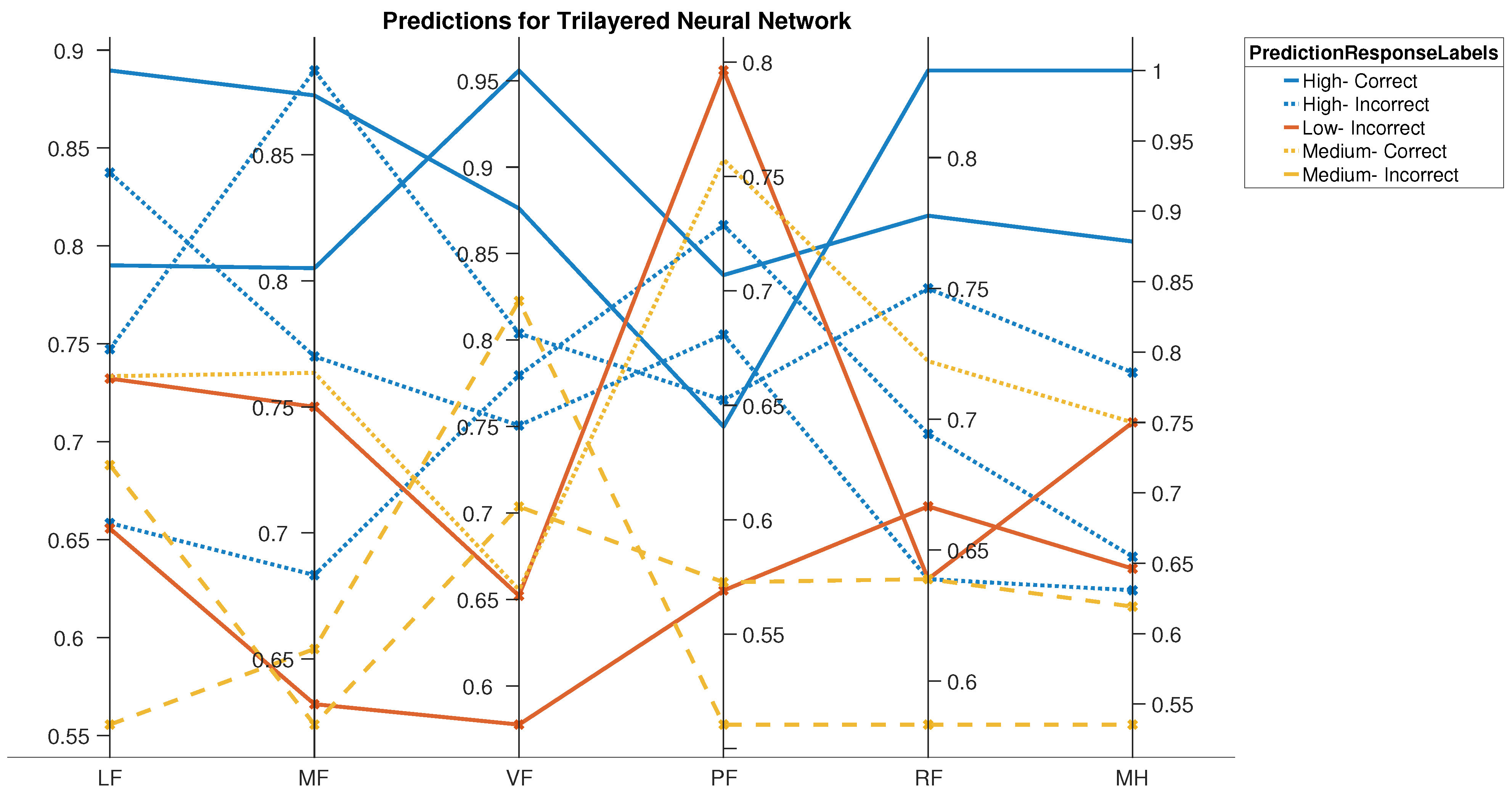
Figure 22.
Validation Predictions: Trilayered Neural Network LM Soft Sensor.
Figure 22.
Validation Predictions: Trilayered Neural Network LM Soft Sensor.
Table 1.
Existing levels of lean manufacturing and manufacturing flexibilities in the surveyed companies [
30].
Table 1.
Existing levels of lean manufacturing and manufacturing flexibilities in the surveyed companies [
30].
| Company No. | LF | MF | VF | PF | RF | MH | LM |
|---|
| 1 | 0.6797 | 0.6715 | 0.7163 | 0.4855 | 0.6111 | 0.6817 | 0.7035 |
| 2 | 0.6144 | 0.6684 | 0.7410 | 0.6389 | 0.7222 | 0.5625 | 0.6896 |
| 3 | 0.7467 | 0.7946 | 0.7467 | 0.6618 | 0.6111 | 0.4021 | 0.8656 |
| 4 | 0.7143 | 0.7184 | 0.7002 | 0.9178 | 0.7778 | 0.8022 | 0.8630 |
| 5 | 0.7319 | 0.7491 | 0.7868 | 0.6523 | 0.7222 | 0.7500 | 0.7694 |
| 6 | 0.6841 | 0.5908 | 0.8294 | 0.5915 | 0.6111 | 0.6462 | 0.7379 |
| 7 | 0.6881 | 0.6240 | 0.7037 | 0.5727 | 0.6389 | 0.6192 | 0.8652 |
| 8 | 0.8636 | 0.8521 | 0.8911 | 0.7858 | 0.7500 | 0.8692 | 0.8852 |
| 9 | 0.7235 | 0.8043 | 0.4272 | 0.6631 | 0.7222 | 0.7146 | 0.7775 |
| 10 | 0.7139 | 0.8270 | 0.8592 | 0.6523 | 0.5000 | 0.6841 | 0.9635 |
| 11 | 0.7979 | 0.7735 | 0.6980 | 0.5247 | 0.5278 | 0.6536 | 0.8384 |
| 12 | 0.7901 | 0.8050 | 0.9559 | 0.7069 | 0.7778 | 0.8785 | 0.9076 |
| 13 | 0.6806 | 0.6601 | 0.7502 | 0.4559 | 0.7778 | 0.4376 | 0.7296 |
| 14 | 0.6532 | 0.6900 | 0.7937 | 0.6573 | 0.6944 | 0.6308 | 0.7751 |
| 15 | 0.7723 | 0.7821 | 0.7345 | 0.6573 | 0.6944 | 0.5505 | 0.8808 |
| 16 | 0.9096 | 0.8260 | 0.8131 | 0.6045 | 0.7222 | 0.6968 | 0.8080 |
| 17 | 0.9073 | 0.8444 | 0.5354 | 0.5727 | 0.6111 | 0.7654 | 0.8155 |
| 18 | 0.6585 | 0.6833 | 0.7796 | 0.7287 | 0.6944 | 0.6546 | 0.6826 |
| 19 | 0.7484 | 0.7334 | 0.7212 | 0.6440 | 0.6111 | 0.7500 | 0.7963 |
| 20 | 0.7473 | 0.8834 | 0.8038 | 0.6523 | 0.7500 | 0.7854 | 0.7879 |
| 21 | 0.6683 | 0.7262 | 0.6942 | 0.8977 | 0.8056 | 0.6158 | 0.7340 |
| 22 | 0.6908 | 0.6400 | 0.6207 | 0.5977 | 0.3611 | 0.3159 | 0.5057 |
| 23 | 0.5658 | 0.6555 | 0.6746 | 0.7105 | 0.6111 | 0.9729 | 0.6340 |
| 24 | 0.7463 | 0.7515 | 0.4737 | 0.7500 | 0.7222 | 0.7500 | 0.7869 |
| 25 | 0.8374 | 0.7700 | 0.7506 | 0.6809 | 0.6389 | 0.6308 | 0.7837 |
| 26 | 0.6557 | 0.6321 | 0.5776 | 0.5691 | 0.6667 | 0.6462 | 0.7369 |
| 27 | 0.7334 | 0.5750 | 0.4796 | 0.5500 | 0.6667 | 0.6817 | 0.5125 |
| 28 | 0.8380 | 0.8442 | 0.7113 | 0.6451 | 0.6111 | 0.5271 | 0.7124 |
| 29 | 0.9193 | 0.8253 | 0.9290 | 0.5616 | 0.7500 | 1.0000 | 0.7217 |
| 30 | 0.5857 | 0.8488 | 0.8680 | 0.5559 | 0.6111 | 0.5000 | 0.9065 |
| 31 | 0.5902 | 0.6631 | 0.6472 | 0.5879 | 0.6667 | 0.7500 | 0.8048 |
| 32 | 0.8341 | 0.6336 | 0.8143 | 0.6773 | 0.6111 | 0.5752 | 0.7340 |
| 33 | 0.8341 | 0.6336 | 0.8143 | 0.6190 | 0.6389 | 0.5752 | 0.7066 |
| 34 | 0.7323 | 0.7500 | 0.6521 | 0.7963 | 0.6389 | 0.7500 | 0.7208 |
| 35 | 0.7014 | 0.7084 | 0.5980 | 0.5832 | 0.6944 | 0.7500 | 0.7081 |
| 36 | 0.5556 | 0.6540 | 0.8226 | 0.5105 | 0.5833 | 0.5354 | 0.6476 |
| 37 | 0.6423 | 0.7445 | 0.8670 | 0.5871 | 0.6667 | 0.7500 | 0.6962 |
| 38 | 0.6697 | 0.7029 | 0.7716 | 0.5858 | 0.6111 | 0.6486 | 0.7743 |
| 39 | 0.7846 | 0.7228 | 0.7015 | 0.6914 | 0.7222 | 0.8715 | 0.7931 |
| 40 | 0.6098 | 0.6448 | 0.6839 | 0.6309 | 0.6944 | 0.6817 | 0.8530 |
| 41 | 0.7777 | 0.6671 | 0.7539 | 0.6856 | 0.6944 | 0.7229 | 0.7078 |
| 42 | 0.7304 | 0.7077 | 0.7112 | 0.7204 | 0.6389 | 0.7500 | 0.5203 |
| 43 | 0.8896 | 0.8735 | 0.8761 | 0.6407 | 0.8333 | 1.0000 | 0.9275 |
| 44 | 0.7335 | 0.7635 | 0.6556 | 0.7573 | 0.7222 | 0.7500 | 0.7714 |
| 45 | 0.6715 | 0.5939 | 0.6772 | 0.6477 | 0.6944 | 0.3751 | 0.7389 |
| 46 | 0.6011 | 0.6567 | 0.6773 | 0.5691 | 0.6667 | 0.7146 | 0.7611 |
| Minimum | 0.5556 | 0.5750 | 0.4272 | 0.4559 | 0.3611 | 0.3159 | 0.5057 |
| Maximum | 0.9193 | 0.8834 | 0.9559 | 0.9178 | 0.8333 | 1.0000 | 0.9635 |
| Average | 0.7266 | 0.7254 | 0.7280 | 0.6442 | 0.6685 | 0.6821 | 0.7618 |
Table 2.
LM levels for classification.
Table 2.
LM levels for classification.
| LM | Level labels |
|---|
| 0.50 to 0.65 | low |
| 0.65 to 0.80 | medium |
| 0.80 to 0.96 | high |
Table 3.
Misclassification cost default settings for all models.
Table 3.
Misclassification cost default settings for all models.
| | | Predicted Class |
|---|
| | | High | Low | Medium |
| | High | 0 | 1 | 1 |
| True Class | Low | 1 | 0 | 1 |
| | Medium | 1 | 1 | 0 |
Table 4.
ANN classification hyperparameters.
Table 4.
ANN classification hyperparameters.
| Model Hyperparameters | Narrow ANN | Medium ANN | Wide ANN | Bilayered ANN | Trilayered ANN |
|---|
| Preset Neural Network | Narrow | Medium | Wide | Bilayered | Trilayered |
| Number of fully connected layers | 1 | 1 | 1 | 2 | 3 |
| Layer Size | 10 | 25 | 100 | 10, 10 | 10, 10, 10 |
| Activation Function | ReLU | ReLU | ReLU | ReLU | ReLU |
| Iteration Limit | 1000 | 1000 | 1000 | 1000 | 1000 |
| Regularization strength (Lambda) | 0 | 0 | 0 | 0 | 0 |
| Standardized data | Yes | Yes | Yes | Yes | Yes |
Table 5.
KNN classification hyperparameters.
Table 5.
KNN classification hyperparameters.
| Model Hyperparameters | Fine KNN | Medium KNN | Coarse KNN | Cosine KNN | Cubic KNN | Weighted KNN |
|---|
| Preset | Fine | Medium | Coarse | Cosine | Cubic | Weighted |
| Number of Neighbors | 1 | 10 | 100 | 10 | 10 | 10 |
| Distance Metric | Euclidean | Euclidean | Euclidean | Cosine | Minkowski (cubic) | Squared Inverse |
| Distance Weight | Equal | Equal | Equal | Equal | Equal | Equal |
| Standardized data | True | True | True | True | True | True |
Table 6.
Tree classification hyperparameters.
Table 6.
Tree classification hyperparameters.
| Model Hyperparameters | Fine Tree | Medium Tree | Coarse Tree |
|---|
| Preset | Fine | Medium | Coarse |
| Maximum number of splits | 100 | 20 | 4 |
| Split criterion | Gini’s diversity index | Gini’s diversity index | Gini’s diversity index |
| Surrogate decision splits | OFF | OFF | OFF |
Table 7.
Discriminant classification hyperparameters.
Table 7.
Discriminant classification hyperparameters.
| Model Hyperparameters | Linear Discriminant | Quadratic Discriminant |
|---|
| Preset Discriminant | Linear | Quadratic |
| Covariance Structure | Full | Full |
Table 8.
Naive Bayes classification hyperparameters.
Table 8.
Naive Bayes classification hyperparameters.
| Model Hyperparameters | Gaussian Naive Bayes | Kernel Naive Bayes |
|---|
| Preset Naive Bayes | Gaussian | Kernel |
| Distribution name for numeric predictors | Gaussian | Kernel |
| Distribution name for categorical predictors | NA | NA |
| Kernel type | NA | Gaussian |
| Support | NA | Unbounded |
Table 9.
Support Vector Machine (SVM) classification hyperparameters.
Table 9.
Support Vector Machine (SVM) classification hyperparameters.
| Model Hyperparameters | Linear SVM | Quadratic SVM | Cubic SVM | Fine Gaussian SVM | Medium Gaussian SVM | Coarse Gaussian SVM |
|---|
| Preset SVM | Linear | Quadratic | Cubic | Fine Gaussian | Medium Gaussian | Coarse Gaussian |
| Kernel Function | Linear | Quadratic | Cubic | Gaussian | Gaussian | Gaussian |
| Kernel Scale | Automatic | Automatic | Automatic | 0.61 | 2.4 | 9.8 |
| Box Constraint Level | 1 | 1 | 1 | 1 | 1 | 1 |
| Multiclass Method | One-vs-One | One-vs-One | One-vs-One | One-vs-One | One-vs-One | One-vs-One |
| Standardized data | True | True | True | True | True | True |
Table 10.
Ensemble classification hyperparameters.
Table 10.
Ensemble classification hyperparameters.
| Model Hyperparameters | Ensemble Boosted Tree | Ensemble Bagged Tree | Ensemble Subspace Discriminant | Ensemble Subspace KNN | Ensemble RUSBoosted Trees |
|---|
| Preset | Boosted Tree | Bagged Trees | Subspace Discriminant | Subspace KNN | RUSBoosted Trees |
| Ensemble Method | AdaBoost | Bag | Subspace | Subspace | RUSBoost |
| Learner type | Decision Tree | Decision Tree | Discriminant | Nearest Neighbors | Decision Tree |
| Maximum number of splits | 20 | 40 | NA | NA | 20 |
| Number of learners | 30 | 30 | 30 | 30 | 30 |
| Learning rate | 0.1 | NA | NA | NA | 0.1 |
| Number of predictors to sample | Select All | Select All | NA | NA | Select All |
| Subspace dimension | NA | NA | 3 | 3 | NA |
Table 11.
ANN Model Results.
Table 11.
ANN Model Results.
| Sr. No. | Model Type | Number of Fully Connected Layers | First Layer Size | Validation | Testing | Training Time (s) |
|---|
| 1 | Narrow Neural Network | 1 | 10 | 30 | 60 | 1.01 |
| 2 | Medium Neural Network | 1 | 25 | 70 | 40 | 0.54 |
| 3 | Wide Neural Network | 1 | 100 | 40 | 60 | 0.71 |
| 4 | Bilayered Neural Network | 2 | 10 | 60 | 40 | 0.75 |
| 5 | Trilayered Neural Network | 3 | 10 | 30 | 80 | 1.02 |
Table 12.
KNN Model Results.
Table 12.
KNN Model Results.
| Sr. No. | Model Type | Number of Neighbors (Default) | Distance Metric | Distance Weight | Validation | Testing | Training Time (s) |
|---|
| 1 | Fine KNN | 1 | Euclidean | Equal | 80 | 20 | 0.95 |
| 2 | Medium KNN | 10 | Euclidean | Equal | 60 | 40 | 0.83 |
| 3 | Coarse KNN | 100 | Euclidean | Equal | 60 | 40 | 0.51 |
| 4 | Cosine KNN | 10 | Cosine | Equal | 60 | 40 | 0.65 |
| 5 | Cubic KNN | 10 | Minkowski | Equal | 60 | 40 | 0.63 |
| 6 | Weighted KNN | 10 | Euclidean | Squared Inverse | 60 | 40 | 0.58 |
Table 13.
Tree Model Results.
Table 13.
Tree Model Results.
| Sr. No. | Model Type | Maximum Number of Splits | Validation | Testing | Training Time (s) |
|---|
| 1 | Fine Tree | 100 | 70 | 60 | 2.62 |
| 2 | Medium Tree | 20 | 70 | 60 | 0.83 |
| 3 | Coarse Tree | 4 | 70 | 60 | 0.76 |
Table 14.
Discriminant Model Results.
Table 14.
Discriminant Model Results.
| Sr. No. | Model Type | Preset | Validation | Testing | Training Time (s) |
|---|
| 1 | Linear Discriminant | Linear Discriminant | 60 | 40 | 0.93 |
| 2 | Quadratic Discriminant | Quadratic Discriminant | Fail | Fail | NA |
Table 15.
Naive Bayes Model Results.
Table 15.
Naive Bayes Model Results.
| Sr. No. | Model Type | Distribution Name for Numeric Predictors | Validation | Testing | Training Time (s) |
|---|
| 1 | Gaussian Naive Bayes | Gaussian | 70 | 40 | 0.86 |
| 2 | Kernel Naive Bayes | Kernel | 60 | 40 | 1.04 |
Table 16.
SVM Model Results.
Table 16.
SVM Model Results.
| Sr. No. | Model Type | Kernel Function | Kernel Scale | Validation | Testing | Training Time (s) |
|---|
| 1 | Linear SVM | Linear | Automatic | 60 | 40 | 1.62 |
| 2 | Quadratic SVM | Quadratic | Automatic | 50 | 60 | 4.47 |
| 3 | Cubic SVM | Cubic | Automatic | 40 | 60 | 1.58 |
| 4 | Fine Gaussian SVM | Gaussian | 0.61 | 60 | 40 | 0.61 |
| 5 | Medium Gaussian SVM | Gaussian | 2.4 | 60 | 40 | 0.53 |
| 6 | Coarse Gaussian SVM | Gaussian | 9.8 | 60 | 40 | 0.51 |
Table 17.
Ensemble Model Results.
Table 17.
Ensemble Model Results.
| Sr. No. | Model Type | Ensemble Method | Learner Type | Validation | Testing | Training Time (s) |
|---|
| 1 | Ensemble Boosted Tree | AdaBoost | Decision Tree | 60 | 40 | 1.23 |
| 2 | Ensemble Bagged Tree | Bag | Decision Tree | 50 | 40 | 1.64 |
| 3 | Ensemble Subspace Discriminant | Subspace | Discriminant | 60 | 40 | 1.5 |
| 4 | Ensemble Subspace KNN | Subspace | Nearest Neighbors | 60 | 20 | 1.08 |
| 5 | Ensemble RUSBoosted Tree | RUSBoost | Decision Tree | 80 | 60 | 1.21 |
Table 18.
Top Seven Models: Result.
Table 18.
Top Seven Models: Result.
| Sr. No. | Model Type | Testing | Validation | Training Time (s) |
|---|
| 1 | Trilayered Neural Network | 80 | 30 | 1.02 |
| 2 | Ensemble RUSBoosted Trees | 60 | 80 | 1.21 |
| 3 | Coarse Tree | 60 | 70 | 0.76 |
| 4 | Quadratic SVM | 60 | 50 | 4.47 |
| 5 | Gaussian Naive Bayes | 40 | 70 | 0.86 |
| 6 | Coarse KNN | 40 | 60 | 0.51 |
| 7 | Linear Discriminant | 40 | 60 | 0.93 |
Table 19.
Precision, recall, and F1 scores of the trilayered neural network soft sensor (testing results).
Table 19.
Precision, recall, and F1 scores of the trilayered neural network soft sensor (testing results).
| | | Prediction Metrics |
|---|
| | | Precision | Recall | F1 Score |
| | High | 1 | 0.5 | 0.67 |
| LM Classes | Low | 1 | 1 | 1 |
| | Medium | 0.67 | 1 | 0.80 |


