
A Bagged Ensemble Convolutional Neural Networks Approach to Recognize Insurance Claim Frauds


Ecole Normale Superieure (ENS), University Hassan II, Casablanca 50069, Morocco
*
Author to whom correspondence should be addressed.
Appl. Syst. Innov. 2023, 6(1), 20; https://doi.org/10.3390/asi6010020
Submission received: 3 January 2023
/
Revised: 22 January 2023
/
Accepted: 23 January 2023
/
Published: 28 January 2023
(This article belongs to the Section Artificial Intelligence)
Abstract
:Fighting fraudulent insurance claims is a vital task for insurance companies as it costs them billions of dollars each year. Fraudulent insurance claims happen in all areas of insurance, with auto insurance claims being the most widely reported and prominent type of fraud. Traditional methods for identifying fraudulent claims, such as statistical techniques for predictive modeling, can be both costly and inaccurate. In this research, we propose a new way to detect fraudulent insurance claims using a data-driven approach. We clean and augment the data using analysis-based techniques to deal with an imbalanced dataset. Three pre-trained Convolutional Neural Network (CNN) models, AlexNet, InceptionV3 and Resnet101, are selected and minimized by reducing the redundant blocks of layers. These CNN models are stacked in parallel with a proposed 1D CNN model using Bagged Ensemble Learning, where an SVM classifier is used to extract the results separately for the CNN models, which is later combined using the majority polling technique. The proposed method was tested on a public dataset and produced an accuracy of 98%, with a 2% Brier score loss. The numerical experiments demonstrate that the proposed approach achieves promising results for detecting fake accident claims.
1. Introduction
The advancement of cutting-edge digital technology in the industries of banking, insurance, communication, and media have introduced many ways to commit financial fraud. To earn unjustified financial gain, financial fraud is committed [1]. Money laundering, corporate fraud, telecom, life insurance, auto insurance, and credit cards are a few examples of financial fraud. According to the agencies, there was a significant loss of revenue as a result of the clients’ fraudulent behavior. The loss was estimated by American agencies to be over USD 80 billion annually [2]. According to a survey by the Australian Insurance Bureau, losses tended to rise in 2013. They exceeded the 2012 figures by more than USD 2 billion [3]. According to research by the British Insurers Association, fraudulent claims are rising daily [4]. These investigations make it clear that false claims are a severe issue that require immediate attention in order to create a mechanism to stop them.
Automobile insurance fraud is the practice of deceiving an insurance provider by requesting financial assistance for vehicle theft or damage using fictitious documentation [5]. The vehicle insurance scam has grown to be one of the main issues for both insurance providers and consumers as recipients of payment in the event of an accident do not always act honestly. Theft or accident planning, submitting a fraudulent application, or other methods of auto insurance fraud are all possible. False data representation makes it difficult to detect fraud [6]. Additionally, there are fewer illegitimate claims than legitimate claims, which contributes to the issue of class inequality. The detecting method is further made more challenging by the imbalanced data. Furthermore, the straight classification of an imbalanced dataset takes time and may produce misclassification errors. Therefore, the precise subset of cases is crucial for the method used to detect vehicle insurance fraud. A powerful method must effectively distinguish between malicious and legitimate situations. Additionally, it ought to reduce the rate of misclassification.
Eliminating the noise and zero-valued data from the initial imbalanced data-set is one of the crucial jobs in many data sets. Eliminating noise is one of the obstacles we face in our work. Another challenge is the hugely imbalanced dataset. To overcome these issues, this article presents an efficient way to eliminate zero-valued data, by analyzing the impact. Further, 1D Convolutional Neural Network (CNN) along with pre-trained CNN models are utilized, which are empowered by bagged ensemble learning techniques to obtain efficient results.
The rest of the paper is organized as follows: Section 2 gives a short review of seminal studies and the state of the art of the problem. Section 3 describes the methodology and the tools used in our approach. Section 4 presents a description of our experimental environment and an analysis of our findings. Finally, Section 5 presents conclusions and future directions.
2. Related Work
Insurance fraud detection has emerged as one of the most popular areas in recent years due to the high costs and losses associated with fraudulent claims.
First interests in fraudulent insurance transactions began in the early 1980s specially in the United States with the appointment of experienced adjusters with special expertise in insurance claim investigations. These units became commonly known as Special Investigation Units or SIUs [7]. Later, in the 1990s, insurers in Canada and Europe also began to recognize the problem of fraud and began to adopt the SIU format to handle suspicious claims [8,9]. By the end of the 20th century corporations had developed extensive internal fraud prevention procedures, with the establishment of fraud investigation bureaus to investigate and prosecute criminals. Auto insurance, particularly personal injury insurance, was systematically investigated for claims patterns related to fraud and excessive medical procedures known as build-ups [10].
The detection of fraudulent insurance claims was conducted manually. In practice, corporate claims management units identify those claims by observing the presence of one or more fraud indicators known as red flags. Claims adjusters are trained to identify those claims that present a set of red flags having historically been associated with questionable claims. The assessment of the likelihood or suspicion of fraud usually relies heavily on claims officers’ observation of anomalies in paper documents. In the following years, the use of pattern recognition technologies was made possible due to the availability of these systematic collections of data.
In recent years, a great number of published research literature has studied applying anomaly detection techniques for detecting insurance fraud. Of those papers, several have focused on machine learning techniques and applications thus making a remarkable impact on the subject. One of the most famous works for detecting fraud in car insurance was a combination of stacking and bagging classifiers, suggested by Phua et al. in 2004. This approach uses a stacked ensemble to select the best base learner method from a group, then applies the bagging technique to an over-sampled data-set [11]. Šubelj et al. proposed an expert system based on the Iterative Assessment Algorithm in 2011 which could detect collaboration among automobile insurance fraudsters, as opposed to other solutions at the time that used networks for data representation and required only unlabeled data for processing [12]. In a similar vein, Xu et al. proposed a neural network combined with a random rough subspace method later in 2011 as means of identifying insurance fraud within the automotive industry by segmenting data-sets into several sub-spaces via rough set data space reduction before training a neural network classifier on all said subspace; results from each classifier are then combined using ensemble strategies [13]. Fuzzy Support Vector Machine (SVM) was used by Tao et al. [14] to assign a dual membership value to each incidence of fraud in relation to the sample callous direction. The classification was carried out based on membership values. To overcome the imbalanced dataset problem, Sundarkumar [15] introduced a different under sampling and outlier identification approach based on one-class SVM and k-reverse nearest neighborhood. Outliers and noisy data were therefore quickly identified. The trimmed dataset was then subjected to basic model applications. Subudhi and Panigrahi published another useful technique for outlier discovery in the mainstream class [3]. They employed clustering with genetic optimization over the mass class. Fuzzy membership values are assigned by FCM, which aids in the identification of significant clusters. The Euclidean distance was calculated from centers of each feature. If the calculated distance exceeds a certain value, the feature is labeled as outlier and eliminated [16].
In the financial sector, fraud can take many forms beside insurance fraud, such as credit card fraud, and money laundering. Convolutional neural networks (CNNs) have been used to detect fraudulent financial transactions in a number of studies. One example of using CNNs for fraud detection is a study by Fu et al. [17]. In this study, the authors used a CNN to detect fraudulent credit card transactions in a dataset of credit card transactions. The CNN was trained on a dataset of both fraudulent and non-fraudulent transactions, and was able to accurately identify fraudulent transactions with high precision and recall out performing state-of-the-art methods. In [18], a CNN-based fraud detection model for online transactions is proposed. The model uses low dimensional, nonderivative transaction data as input and consists of a feature sequencing layer, four convolutional and pooling layers, and a fully connected layer. Experimental results show that the model outperforms the existing CNN for fraud detection. Most recently, in [19], authors proposed a combination of CNN and LSTM. The model was able to reduce the need of complex feature extraction processes that often rely on domain experts in traditional machine learning algorithms.
In conclusion, the detection of fraud in insurance claims is a well-researched area. It appears that machine learning paradigms, particularly convolutional neural networks (CNNs), outperform traditional methods. It is important to note that the effectiveness of these methods for fraud detection depend on the quality of the training data and the specific details of the model architecture. Additionally, the imbalanced nature of data is a current challenge in the field. Consequently, in the work we propose a combination of a 1D Convolutional Neural Network and pre-trained CNN models enhanced with a bagged ensemble learning techniques to boost the detection effectiveness and achieve maximum accuracy. The main contributions of this article can be summarized as following:
- We used an analysis technique for cleaning and improving the quality of the chosen dataset.
- We proposed a 1D Convolutional Neural Network along with the use of pre-trained CNN models.
- We used a bagged ensemble learning based architecture to boost the model performance.
- We assessed the performance of our proposed model using different paradigms and performance ratios.
3. Materials and Methods
3.1. Deep Convolutional Neural Network
A deep convolutional neural networks (DCNN) are a type of artificial neural networks that are specifically designed for image recognition tasks where they have achieved excellent success. It is called “deep” because it has a large number of layers, typically several dozen or more, that are stacked on top of each other. Each layer in a DCNN consists of a set of filters that are applied to the input image to extract different features. These features are then passed through non-linear activation functions, which allow the network to learn more complex patterns in the data. The output of a DCNN is a prediction of the class or label to which the input image belongs. DCNNs have been successful in a wide range of image recognition tasks [20] and are now widely used in many applications such as object detection [21], facial recognition [22], and medical image analysis [23].
Deep convolutional neural networks (DCNNs) have been used for fraud detection in a variety of contexts (see Section 2). For example, DCNNs have been applied to detecting fraudulent credit card transactions by learning to recognize patterns in transaction data that are indicative of fraud. DCNNs have also been used to detect fraudulent insurance claims by analyzing images of damage or injuries and learning to distinguish between genuine and fake claims [24]. In both cases, the goal of using a DCNN for fraud detection is to be able to automatically learn patterns in the data that are indicative of fraud, without the need for manual feature engineering or domain expertise. This can make DCNNs a powerful tool for detecting fraud in a large and complex dataset.
In order to build one class, CNNs learn from larger datasets using several models. These models’ capacity may be adjusted by varying the depths and breadth, allowing the models to accurately represent various types of images. CNNs have fewer parameters and connections than feedforward neural networks with the same number of layers, making them simpler and more practical to test and train. Most of the proposed pre-trained CNN models usually work with image data, where data has three channels, i.e., RGB. To work with time-series data, either the network needs to be modified at each layer, or the input data must be mapped to present a shape, similar to images. In this regard, the following pre-trained models are selected and analyzed for this work.
3.1.1. InceptionV3
Google came up with this model by expanding the prior model, InceptionV1 [25]. InceptionV3 is used in a variety of image classification and anomaly detection problems, such as cell classification [26], pulmonary image classification [27], flower classification [28], etc. InceptionV3 also used a 1D model, in [29]; the authors compared several deep one-dimensional convolutional neural network architectures on the same 1D data, and showed that 1D InceptionV3 outperforms XGBoost, a non-deep machine learning model, as well as other traditional detection algorithms.
Convolutional layers with filter widths ranging from 11 to 55 are present in this model along with numerous highly configurable inception blocks. The Inception model went much deeper than all other architectures while having fewer parameters than earlier CNN models. The average pooling layer with the name “avg pool” layer gives 2048 features for one input, but the input size for this model is a 3D data.
3.1.2. ResNet-101
The ResNet model was first introduced by He et al. [30]. Afterward Microsoft came up with the Resnet-101 technique by employing the skip connections idea for quicker convergence [31]. ReseNet-101 is known to give very good results in anomaly detection tasks [32,33].
This model’s depth allows it to train more quickly than any other model that has been previously suggested because it incorporates batch normalization methodology to prevent overfitting. A linear layer called “fc1000” is used in place of the traditional fully connected layers to reduce the number of parameters. This network’s input is 3D data, and its “flatten 0” Flatten Layer extracts 2048 features from an input while its “fc1000” layer extracts 1000 features.
3.1.3. AlexNet
This model, which was suggested as a larger and deeper model than LeNet, won the LSVRC competition in 2012 by outperforming all other traditional techniques to computer vision and machine learning in terms of accuracy [34]. These findings demonstrated a significant advancement in classification and recognition tasks. The fully connected layers ’fc6’ and ’fc7’ each extract 4096 features from the usual input of 3D, whereas ’fc8’ extracts 1000 features from a single input [35].
A thorough analysis of architectures reveals that each model’s layer organization is remarkably repetitive. There are numerous layers that are unnecessary and only add to the complexity of the corresponding models. On all three of the chosen CNN models, this observation is made. In order to achieve the same performance with less layers, these three pre-trained CNN models are also tuned for time-series data in this work in addition to the unique, lightweight, and minimal 1D CNN model that is proposed. By including a Data Reshape layer, all of these CNN models’ filters, inputs, outputs, and operations are converted from 3D data to 1D data. In this article’s ablation study, the total number of repeated layers for each pre-trained CNN model is also examined and described.
3.1.4. Minimized 1D CNN
After the analysis of pre-trained models, a minimized, yet efficient sequential network is proposed as a productive method of extracting time series data’ deep features. The main idea of this model is to obtain better results with a CNN architecture having minimal complexity. The proposed network only has 19 layers in total, including one output layer, two max pooling, dropout, and fully connected layers, four convolutional, batch normalization, and ReLU layers, and four of each. This model has fewer layers then AlexNet model yet performs better than all three pre-trained CNN models. The proposed 1D CNN model’s parameters, inputs, and outputs are all included in Table 1 thorough overview.
3.2. Bagged Ensemble Learning
Ensemble learning presents a comprehensive, efficient and meta-approach to machine learning that tries to enhance predictive capabilities by blending the predictions from several models. Although there are many ensembles we may build to solve our predictive modeling problem, bagging, stacking, and boosting are the three strategies that dominate the ensemble learning space. Bagging entails averaging the predictions from many models that have been fitted to various samples of the same dataset. This typically entails training each model on a distinct sample of the same training dataset while employing a single machine learning method, which is nearly invariably an unpruned algorithm.
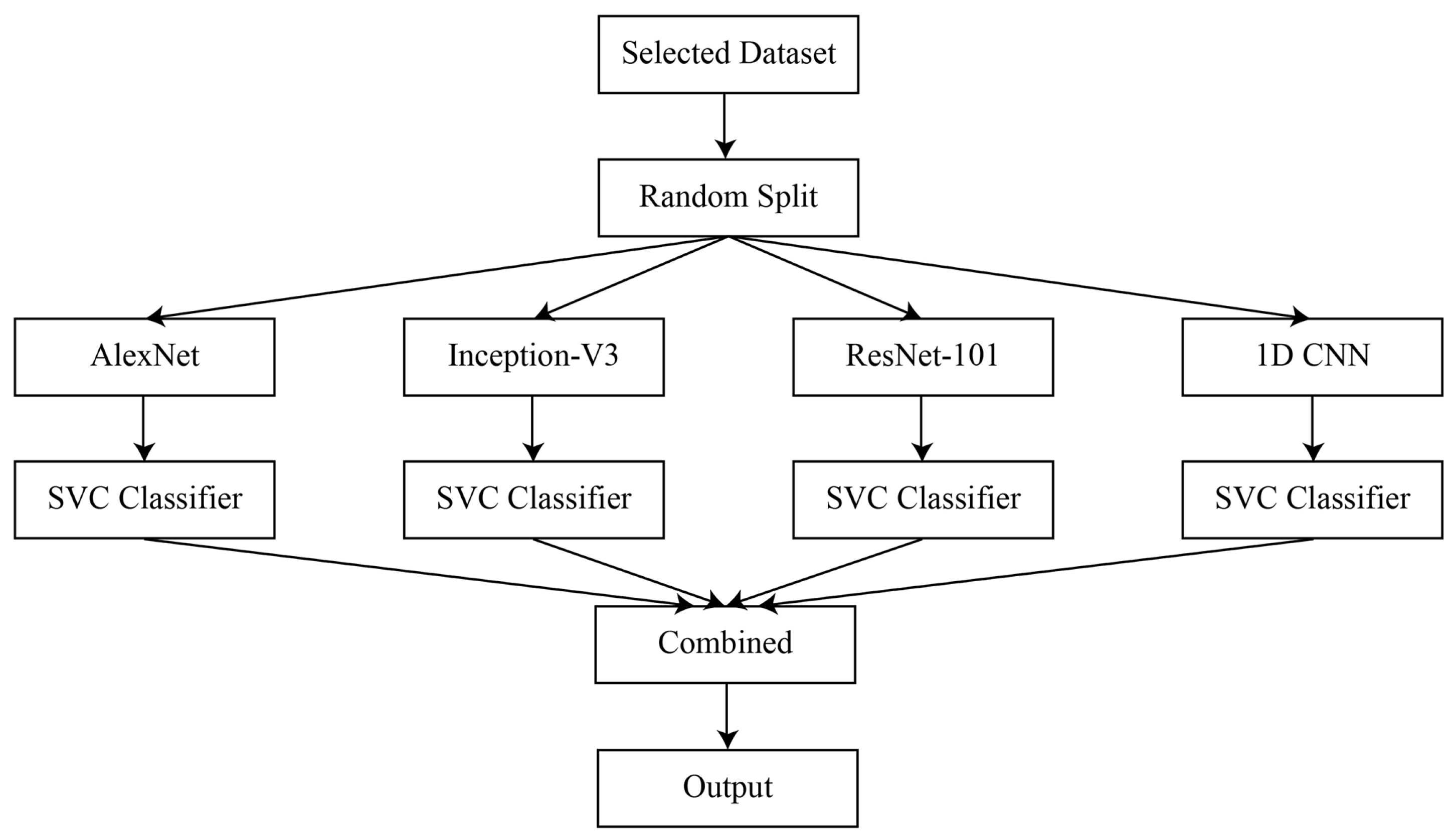
The forecasts from the ensemble members are combined using majority polling. The whole procedure depends on how each dataset model is made to train ensemble members. The dataset is split up into individual samples for each model. These samples are chosen at random, albeit with replacement, from the dataset. If a row is chosen, replacement means that it is returned to the training dataset in case it is chosen again in the same training dataset. This implies that for a specific training dataset, a row of data may be chosen 0 times, 1 time, or many times. Figure 1 shows the structure of the proposed Bagged Ensemble Learning-based model.
3.3. Performance Metrics
In this contribution a total of seven metrics are selected to assess the performance of our proposed model namely, Accuracy, Recall Score, Precision Score, Balanced Accuracy, F1 Score, Brier Score Loss, and ROC AUC Score; Each metric is described briefly in the following:
Accuracy (Acc): The accuracy is defined as the ratio of correctly predicted to total number of instances; it is calculated using the following formula:
where and are the number of correctly predicted positives and negatives, respectively, while and are the number of falsely predicted positives and negatives, respectively.
Recall Score (RS): Recall is defined as the ratio of correctly predicted positive instances to the total number of positive instances; it is calculated using the following formula:
Precision Score (PS): Precision is defined as the ratio of correctly predicted positive instances to the total number of predicted positive instances; it is calculated using the following formula:
Balanced Accuracy (BAcc): Balanced accuracy is defined as the average of recall and precision; it is calculated using the following formula:
F1-score (F1): F1-score is defined as the harmonic mean of precision and recall; it is calculated using the following formula:
Brier Score Loss (BSL): Brier score loss is a proper scoring rule which quantifies the accuracy of probabilistic predictions; it is calculated using the following formula:
where is the predicted probability of the i-th instance being positive and is its actual class label.
ROC AUC Score (AUC): ROC AUC score is the area under the ROC curve; it quantifies the ability of the model to distinguish between positive and negative classes.
3.4. Comparaison Paradigms
Based on the literature, we have selected popular machine learning and statistical classifiers which are widely used in fraud detection systems. To test the effectiveness of our proposed model, those binary classification methods are used for a performance comparison. XGBoost Classifier, Decision Tree, KNeighbors, SVC, Gaussian Process, Random Forest, MLP, AdaBoost, Quadratic Discriminant Analysis, and GaussianNB are all among the ten classifiers employed in this study. A brief description of each classifier is in the following:
XGBoost Classifier(XGB): XGBoost is a gradient boosting system developed by Tianqi Chen. The system was originally created to improve speed and model performance. XGBoost has become the most popular machine learning system for structured or tabular datasets. It implements machine learning algorithms under the Gradient Boosting framework. XGBoost, under the Gradient Boosting framework, provides a parallel tree boosting algorithm (also known as GBDT or GBM) that is fast and accurate. The same code can be used on different distributed environments (such as Hadoop, SGE, MPI) to solve problems with billions of examples. Due to the size of data in insurance claim fraud problems and the imbalanced nature of data, XGBoost showed promising results in this area [36]. XGBoost based model can outperformed other methods such as Support Vector Machine, Random Forest and Logistic Regression in highly imbalanced datasets [37].
Decision Tree (DT): A decision tree is a type of flowchart that uses a tree-like structure to show the possible outcomes of an event or problem. The different branches of the tree represent different options or choices, and each leaf node represents a final outcome (such as success or failure). The root node is the starting point for the decision tree; it learns which attribute value to partition on based on previous data. Partitioning the tree in this way is known as recursive partitioning. In problems with highly imbalanced data, DT can perform slightly better than other algorithms. In [38], the authors used a publicly available automobile insurance fraud detection dataset and demonstrated that DT slightly out performances Support Vector Machine (SVM) and Artificial Neural Network (ANN).
KNeighbors: The k-nearest neighbors algorithm (k-NN) is a non-parametric method that can be used for both classification and regression. For each new data point, the k closest training examples are found in the feature space. The output then depends on whether k-NN is being used for classification or regression. In the literature KNN seems to perform better than other algorithm in anomaly and fraud detection tasks. One example is in [39] where the authors examined the performance of 3 machine learning models implemented on credit card transactions to identify fraudulent behavior. The authors performed a comparative analysis using K-NN, Naive Bayes, and Logistic Regression trained on a credit card dataset designed by European cardholders containing 284,807 transactions. The finding of the comparative analysis shows that K-Nearest Neighbor outperformed LR and NB techniques.
SVM: Support Vector Machine is one of the most widely used algorithm in financial fraud detection [40]. It is a supervised learning algorithm that can be used for both classification and regression tasks. The main idea of SVM is to create a line or decision boundary that can best segregate n-dimensional space into classes, so that new data points can be easily placed in that space. This line is called a decision boundary.
Gaussian Process (GP): A Gaussian process is a generalization of the multivariate normal distribution which applies to any collection of random variables, provided that only a finite number of them are considered at any one time. GP is a powerful model that can be used for anomaly detection in machine learning problems. One of the key advantages of GP is its ability to model non-linear and complex relationships in the data, which makes it well-suited for detecting anomalies in high-dimensional data [41].
Random Forest (RF): Random Forests are an ensemble learning method that constructs a multitude of decision trees at training time. For classification tasks, the forest outputs the class that is the mode of the classes of the individual trees. For regression tasks, the Forest outputs the mean prediction of the individual trees. The Random Forest algorithm has demonstrated its proficiency in identifying fraudulent activities in financial and credit card transactions [40]. One of the key benefits of utilizing this algorithm is its capability to process high-dimensional and imbalanced datasets, which are prevalent in fraud detection scenarios [42]. Furthermore, it gives an insight into the most vital features for fraud detection by providing feature importance information.
Multilayer perceptron (MLP): A multilayer perceptron is a type of artificial neural network that can be used for supervised learning. It consists of an input layer, hidden layers, and an output layer. The hidden layers are composed of neurons with a nonlinear activation function. Multilayer perceptrons are commonly used for tasks such as classification and regression. MLP has been used in various fraud detection problems, such as credit card fraud detection and financial fraud detection [40]. However, MLP requires a large number of labeled data to train effectively, which may not always be available in fraud detection problems. Additionally, it can be sensitive to noise, and the choice of architecture, activation functions, and the number of hidden layers are also important for obtaining good results.
AdaBoost: Adaptive Boosting is a machine learning meta-algorithm that can be used to improve the performance of other types of learning algorithms. It does this by combining the outputs of the other learning algorithms (known as ’weak learners’) into a weighted sum that represents the final output of the boosted classifier. AdaBoost is adaptive in that it adjusts subsequent weak learners to favor those instances which were misclassified by previous classifiers. Adaboost was proposed by Yoav Freund and Robert Schapire [43] and won the 2003 Gödel Prize for their work. A study by Randhawa et al. [44] aimed to detect credit card fraud using machine learning algorithms, taking into account the sensitivity of working with real-world credit card information. The research employed a variety of machine learning techniques, including standard neural networks and deep learning models. The study started by testing standard algorithms such as SVM, NB and DL, and then implemented hybrid methods by combining AdaBoost and majority voting techniques. The proposed method achieves good accuracy rates in detecting fraud cases.
Quadratic Discriminant Analysis (QDA): Quadratic discriminant analysis is a statistical classification technique, it is a variant of Linear Discriminant Analysis (LDA). QDA makes assumptions about the distribution of data in each class, and is therefore considered a generative model.
GaussianNB: Naive Bayes (NB) is widely used in financial fraud problems [40]. GaussianNB is based on the assumption that the data are distributed according to a Gaussian distribution, which means that it is clustered around a mean value. The classifier assigns each data point a class label based on the class with the highest probability of occurring.
3.5. Dataset
According to multiple surveys published in the Coalition Against Insurance Fraud website [45], nearly one in four Americans believe that defrauding insurance is acceptable. If they knew they could get away with it, about one out of every ten Americans would commit insurance fraud. Nearly one in four Americans believe that defrauding insurance is acceptable. One in ten persons feel that it is acceptable to file claims for goods that are not lost, damaged, or destroyed, or for personal injuries that never happened. Two out of every five individuals say they are “not very likely” or “not likely at all” to report someone for defrauding an insurance company. A total of 29 percent of Americans say they would not report an insurance scam committed by a friend. The real dataset used in this reseach study was released by an American insurance company, has 15,420 items with various parameters, such as accident information, automobile model, insurance type, and fault, among others. This dataset’s target class, FraudFound, determines whether a submitted application is fraudulent.
There are a total of 32 columns in this dataset, which provide different types of information regarding the claim. Out of these columns, the policy number is just a unique number for each entry, which represents nothing. Thus, this column is not considered important to decide the fraudulent case. The dataset is further analyzed to find unique values against each column. One row has been purposefully removed because it was seen that columns such as MonthClaimed and DayOfWeekClaimed, contain zeros. The Age column is evaluated in the following phase, where a total of 319 rows had a zero value. Instead of utilizing a mean value, the aim is to impute the data logically, by examining the AgeOfPolicyHolder field.
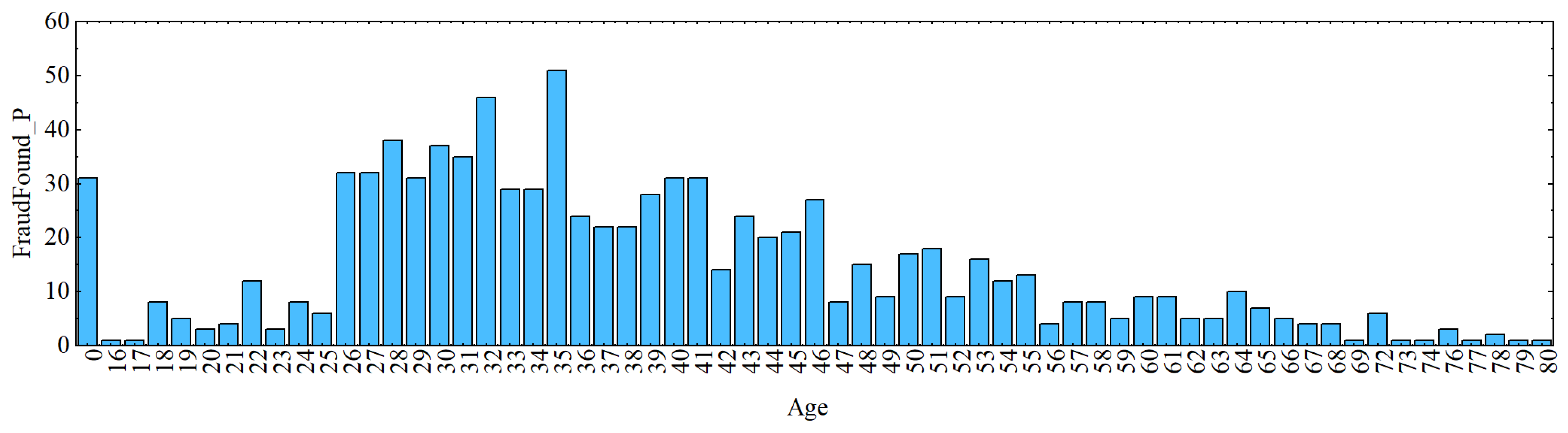
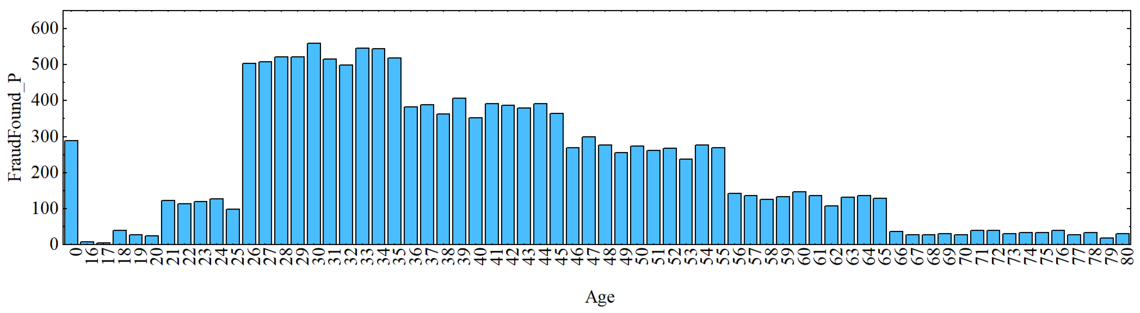
AgeOfPolicyHolder zero values are all between 16 and 17 years old. As a result, a further investigation is performed to see if the subjects with age zero were of legal driving age or not. It was identified that the mean age is lower than the range of each AgeOfPolicyHolder until the 36 to 40 range. This finding revealed that while there are a majority of guilty cases, not all of them are; therefore, we cannot draw the conclusion that zeros are minors (under driving age). As a result, it is assumed that 16 years old is the minimum legal driving age. A graphic depiction of the association between age and fraud is shown in Figure 2 and Figure 3.
The previous imputation technique produces a lot of noise, as the preceding image illustrates. Therefore, analysis is conducted by examining the dataset’s representation of the 319 indicated values. Following the investigation, it was also shown that just 3.36% of fraud cases started at age 0 overall. Given that they are a minority, it was chosen to delete those values from the dataset so that they wouldn’t affect the suggested algorithm’s effectiveness. By eliminating the columns with age values 0, the rows with values 0 in the MonthClaimed and DayOfWeekClaimed columns are also removed.
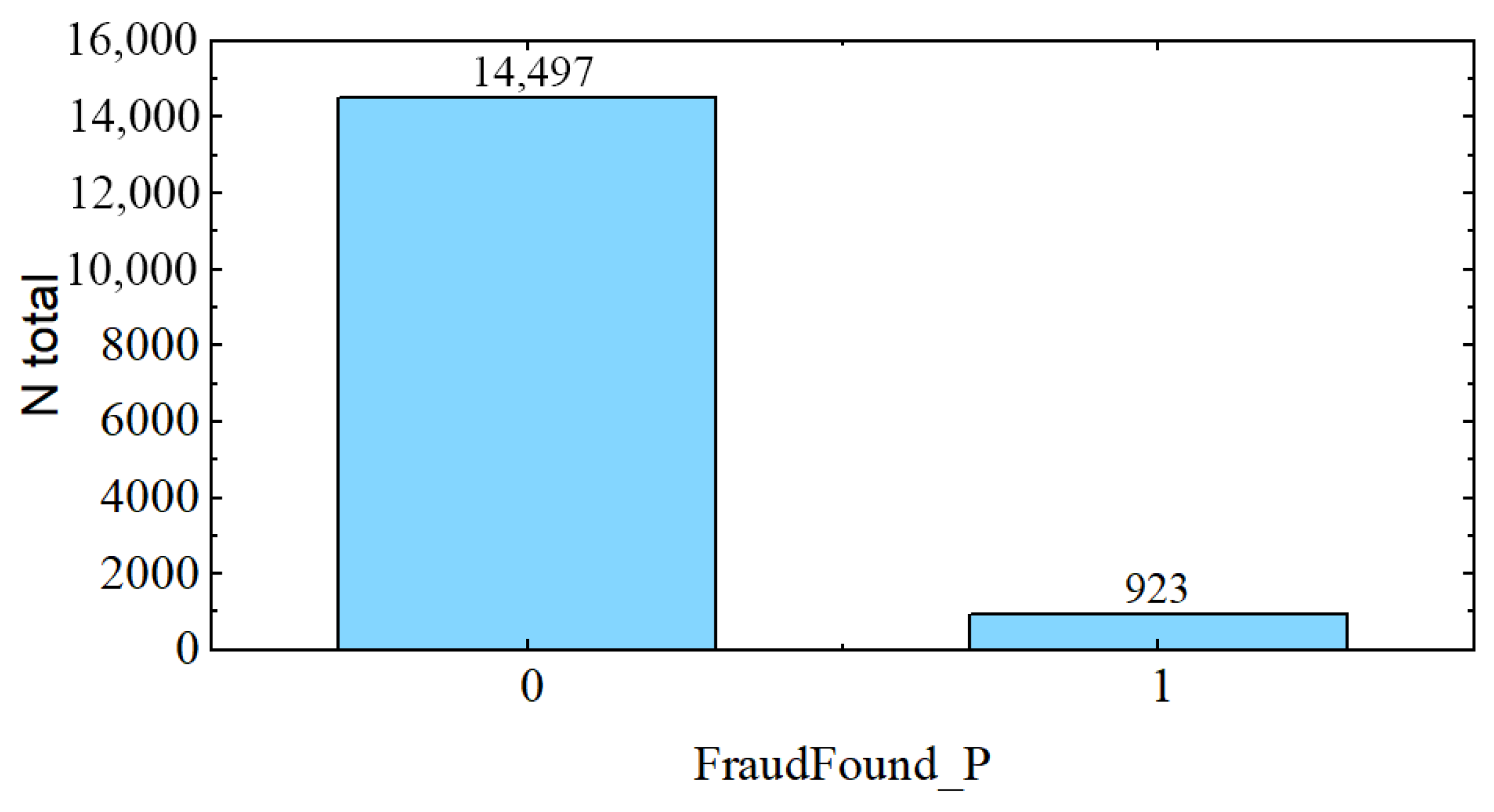
It is then noticed that PolicyType is a string created by concatenating BasePolicy with VehicleCategory. The type of insurance is a perfect fit; however, the car type is not. So that a proper comparison between VehicleCategory and BasePolicy can be conducted, two new columns are created from PolicyType. Following this, the initial BasePolicy column and the newly generated BasePolicy2 column are compared, and there are no mismatches discovered. This results in the BasePolicy2 column being identical to the BasePolicy column. However, a total of 4849 discrepancies are discovered when the VehicleCategory is compared to the VehicleCategory2. As a result, it was decided to remove the original PolicyType column and keep the newly created columns, BasePolicy and VehicleCategory. It is obvious that there is a difference in the numbers of sedans and sports cars, but it is difficult to draw conclusions because it is unknown what type of vehicle falls into each category. The next observation is that the dataset has an imbalanced variable to be predicted, as shown in Figure 4, fraud rate is only 5.91% of the whole data.
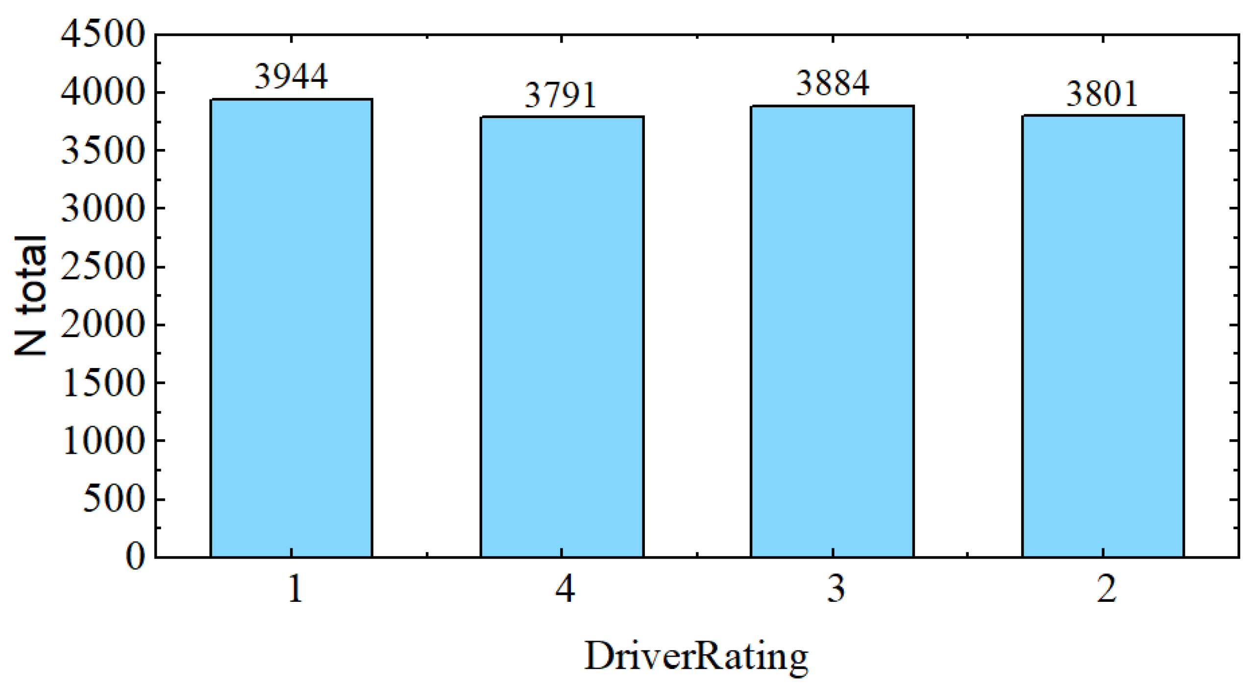
We cannot infer that DriverRating is correlated with the number of accidents, that is, if someone with a rating of 1 is less likely to have an accident than someone with a rating of 4. This is because DriverRating is uniformly distributed, as seen in Figure 5.
Another interesting finding is that fraud in All Perils insurance is substantially more frequent (9.84%) than it is in Collision (7.29%) and Liability (0.71%). Additionally, analysis shows that 6.21% of fraudulent individuals were men and 4.34% were women.
3.6. Experimental Setup
These experiments are all performed using Google Colaboratory. Different split ratios are tested during the experiments, but the 70–15–15 strategy for training, validation and testing yields the best results. This split ratio is performed using a stratified random selection of rows, which is helpful to train distinct models on the same dataset while preserving the ratio of the aimed class. Mini batch size of 32, initial learning rate of 0.002, and a total of 70 epochs are used for the 1D CNN model. Further detail about the fine tuning of the learning parameters is shown Section 4.2.
4. Experiments and Analysis
This section summarizes the outcomes of various experiments that were carried out throughout implementation.
4.1. Experiments
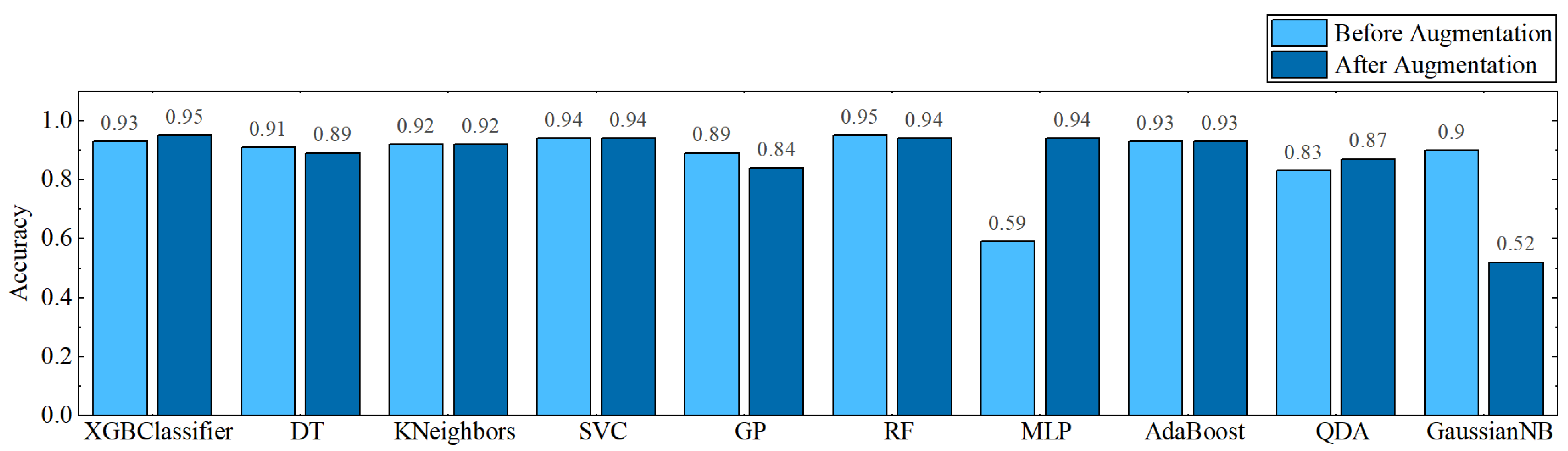
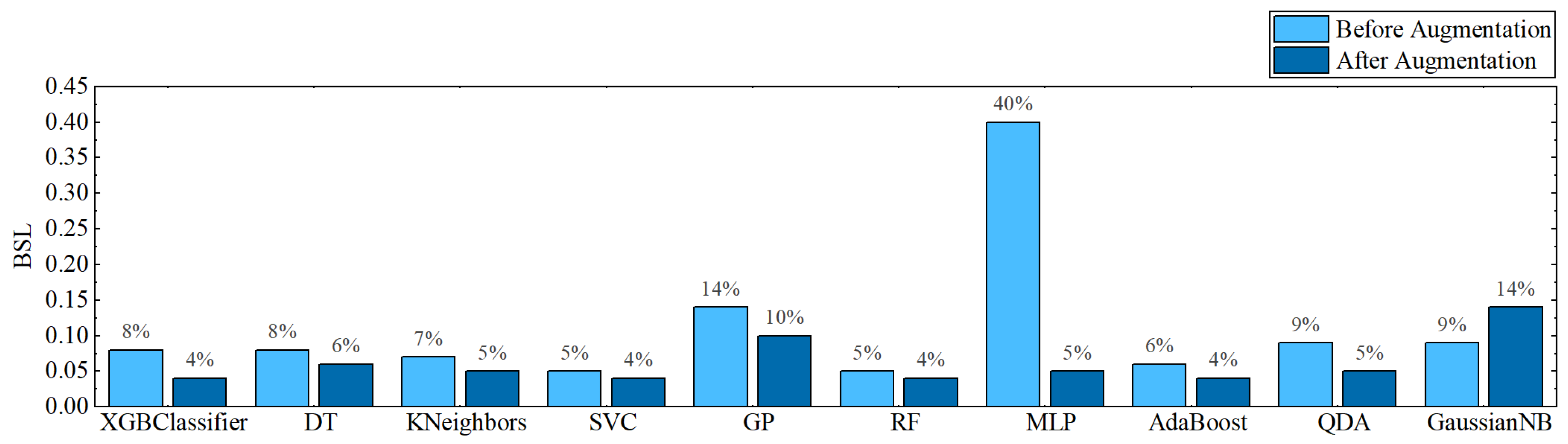
In the first experiment, all classifiers are assessed using a set of performance metrics on data before cleaning and augmentation. The Random Forest classifier in this experiment was able to reach a maximum accuracy of 95% with a balanced accuracy of 50%. SVC has the second-best accuracy of 94% (see Figure 6); however, its balanced accuracy is only 43% (see Figure 7). The lowest BSL recorded against SVC is merely 5% (see Figure 8).
Data cleaning and augmentation is taken into account in the second experiment to make the dataset more realistic. Firstly, the dataset was modified by deleting rows with empty or zero values, as was explained in Section 3.5. Secondly, the Training dataset has an imbalance in favor of the No FraudFound class, with only a small proportion of data points belonging to the FraudFound class (Figure 4). This can cause issues when training our models, as the model may be biased towards the majority class, and have difficulty accurately identifying the minority class. To address this, we use a simple random resampling technique to balance the dataset. This is conducted by generating new data points for the minority class for training sets. By over-sampling the minority class, we can ensure that the model is exposed to a more diverse set of data during training, and is less likely to overfit to the majority class.
Most of the classifiers’ accuracy increased during this exercise (see Figure 6). Additionally, the balancing accuracy was enhanced (see Figure 7), and BSL was greatly decreased (see Figure 8). In this trial, XGBClassifier achieved the greatest accuracy of 95% with a balanced accuracy of 70% and 4% BSL. SVC, with a balanced accuracy of 65% and a BSL of 4%, achieves the second-best accuracy of 94%.
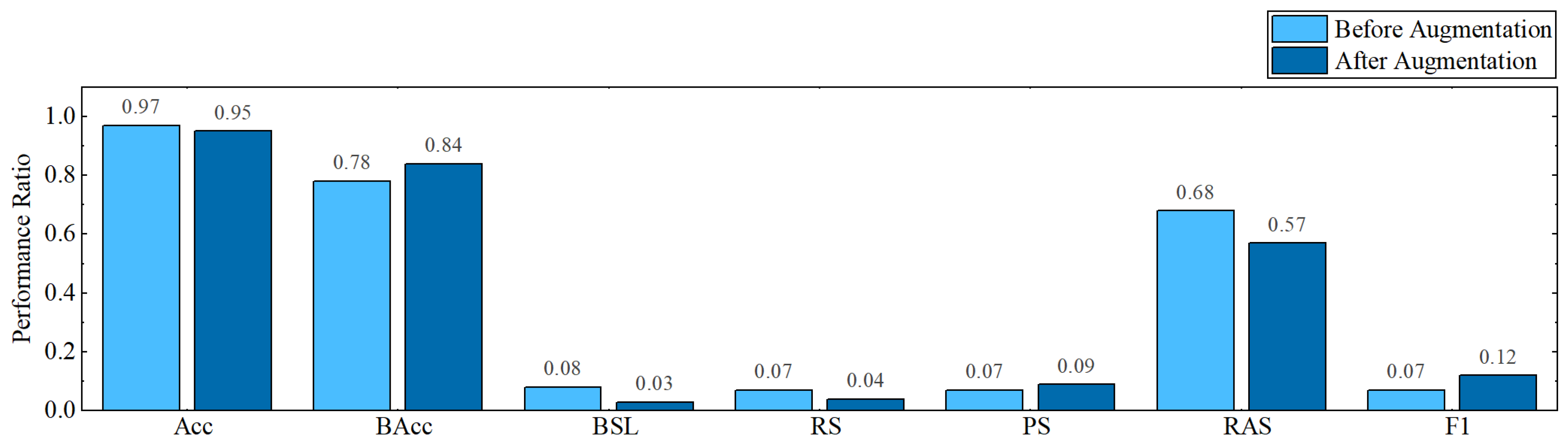
The last experiment makes use of the proposed 1D CNN model. Before and after the augmentation process, the 1D CNN model is tested; the fully_connected_1 layer’s feature has the highest accuracy. All of the classifiers that were considered for this experiment are evaluated, but only the SVC classifier’s findings are shown in Figure 9 because they were superior to those of the other classifiers. When the proposed CNN model is fed a dataset without any augmentation, it achieves 97% accuracy, 78% balanced accuracy, and 8% BSL. When comparing the results after the augmentation phase to the results before augmentation, the overall accuracy is dropped to 2%, but the balanced accuracy is obtained at 84%, and BSL is reduced to 3%.
4.2. Ablation Analysis
This section discusses different experiments, which were conducted before selecting the optimal arrangement/values for specific variables. To reduce the experimental section of this article, this section only presents the results on the proposed 1D CNN model after augmentation. The most important factor is the data split ratio. It is mentioned in Section 3.6, that 70–15–15 split ratio for training, validation and testing has achieved maximum results. In this study, we used a stratified, random approach to split the dataset in the three different sets. The data are shuffled randomly, then split into different sets while maintaining the ratio of fraud and non-fraud cases. The randomness of the splits is an important aspect in this study as it allows each of the used models to be trained on a different set. Although the performance of the model may vary slightly with each random split, the difference is minimal. Each random split is conducted five times and the mean values are rounded to the hundredths and presented in Table 2.
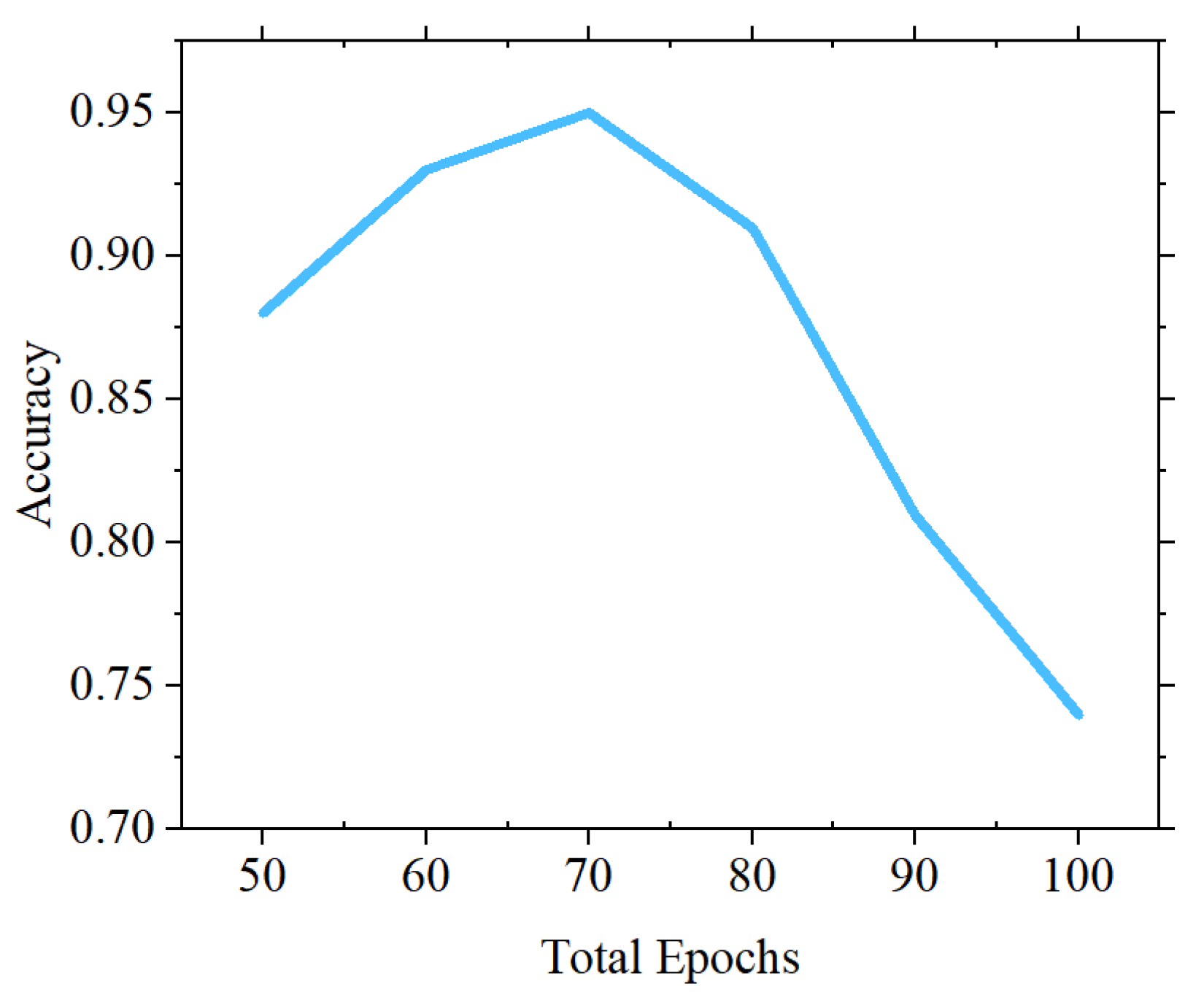
The initial learning rate and total epochs are second crucial aspects. The CNN model’s initial learning rate establishes its character, and total epochs effectively train the model. Due to the imbalanced nature of the dataset, incorrectly setting either of these two variables may result in under or overfitting. Considering the class distribution of the dataset, it is desirable to consider an early stopping strategy using all possible data for training.
The approach followed in this work is to consider an array of total epochs and grid search the model effectiveness of on the different values. Figure 10 shows the impact of the chosen values on the accuracy of the model, the experiment shows that the model is prone to over fitting, and the best performance is given on a 70 epochs training.
The furthermore improve the performance of the models several value of learning rates are tried. As indicated in Table 3, an initial learning rate of 0.002 gives the best accuracy.
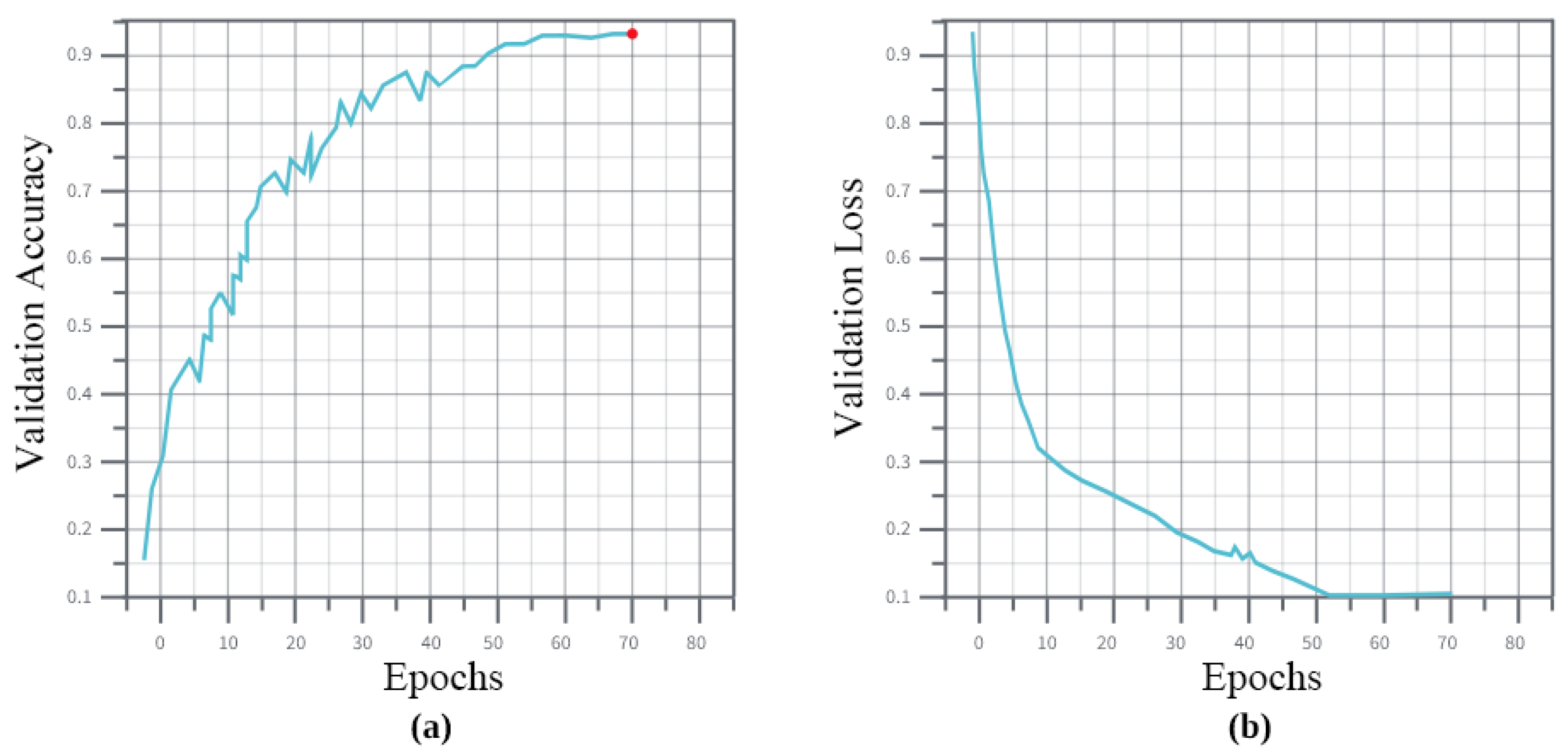
Figure 11 show the models performance for a fixed epoch of 70 and a 0.002 learning rate on the validation set. The loss stabilized after 50 epochs, but gained more accuracy after 20 more epochs.
The last and most important analysis is the impact of the proposed 1D CNN model as compared to existing pre-trained CNN models. During this analysis, two things are considered; first the minimization of pre-trained models; and second the conversion of pre-trained CNN models to work on 1D data. When the pre-trained models are selected, their architectures are thoroughly investigated. During the process, it was found that all selected CNN models contained redundant layers, which if removed, will not impact the outcome, specifically in the case of 1D data. During this process, when AlexNet was analyzed, it was noted that three blocks of convolutional layers and max pooling layers appeared three times, with different filter sizes for convolutional layers, every time. During the analysis of InceptionV3, a total of seven blocks were identified with similar layers, i.e., convolutional, average pooling and concatenation. In the Resnet-101 architecture, layers were connected to next layers as well as convolutional layers were also connected with other convolutional layers. There were seven repeated blocks identified in the Resnet-101 model.
The next step of this analysis is to convert these pre-trained CNN models in a way that 1D data can be processed. For this, all the layers having 4D input were transformed to work with the 3D inputs. This is conducted by adding a Reshape layer, which takes 4D data and manipulates it into 3D data. Table 4 compares the results of a pre-trained model on selected dataset, while using full and partial architectures. It is noteworthy that the columns 2, 5 and 7 of Table 4 present the total number of selected repeated blocks in each model. The rest of the models are kept the same, apart from converting 4D data into 3D data.
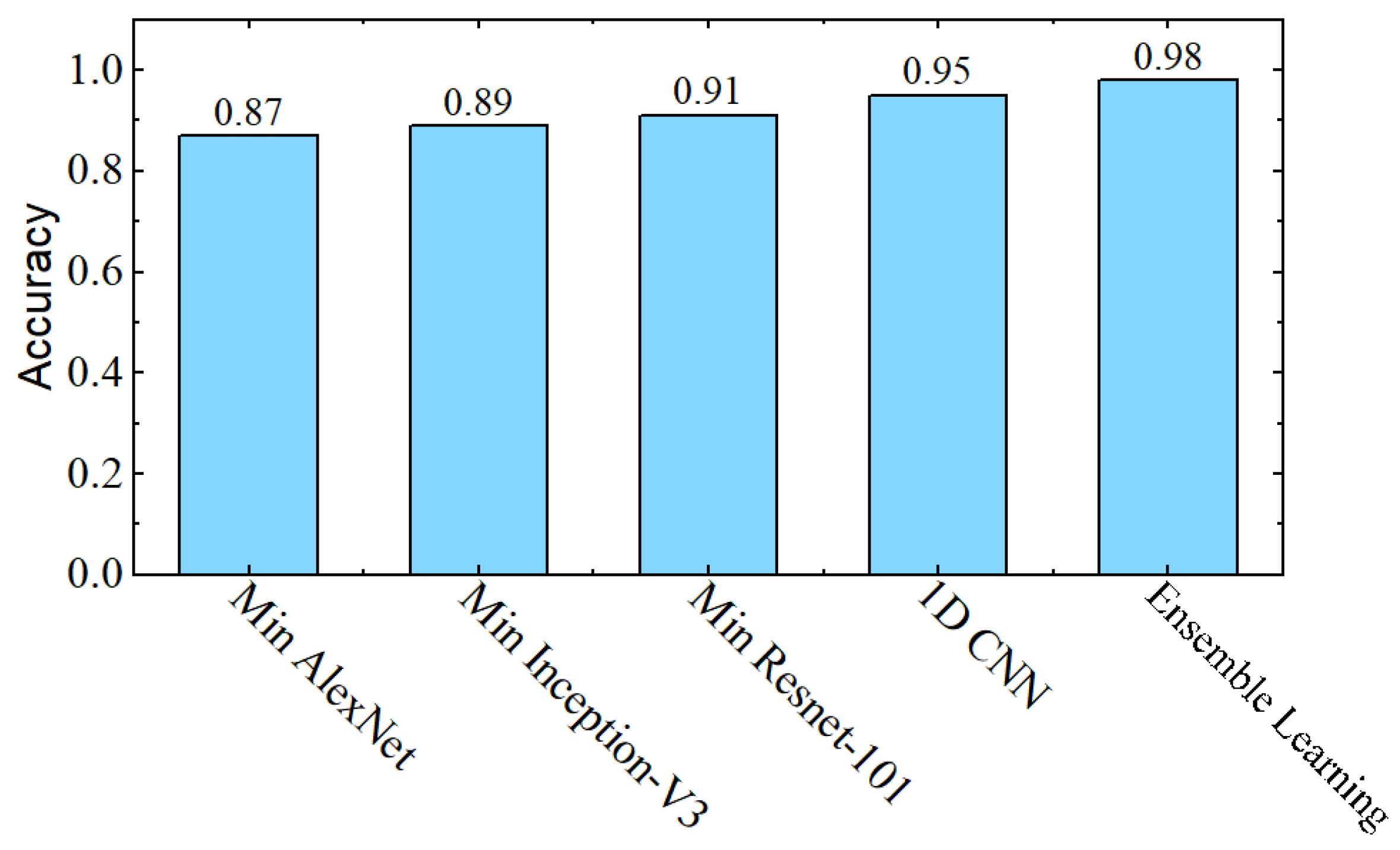
In the second analysis, minimized pre-trained CNN models are compared with the proposed CNN model. The initial learning rate, total number of epochs and environment is kept the same for all these models. Figure 12 compares the result of pre-trained CNN models and proposed 1D CNN model.
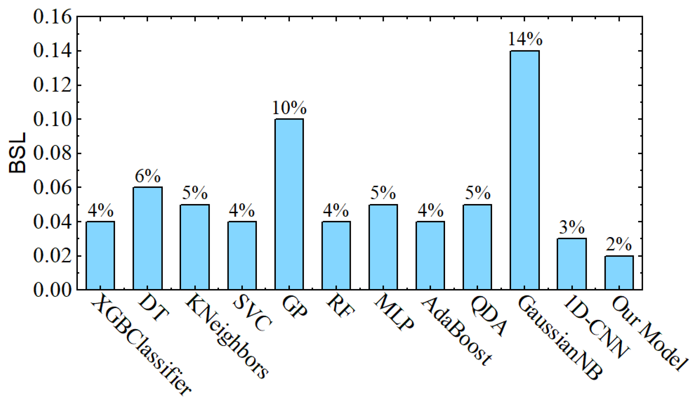
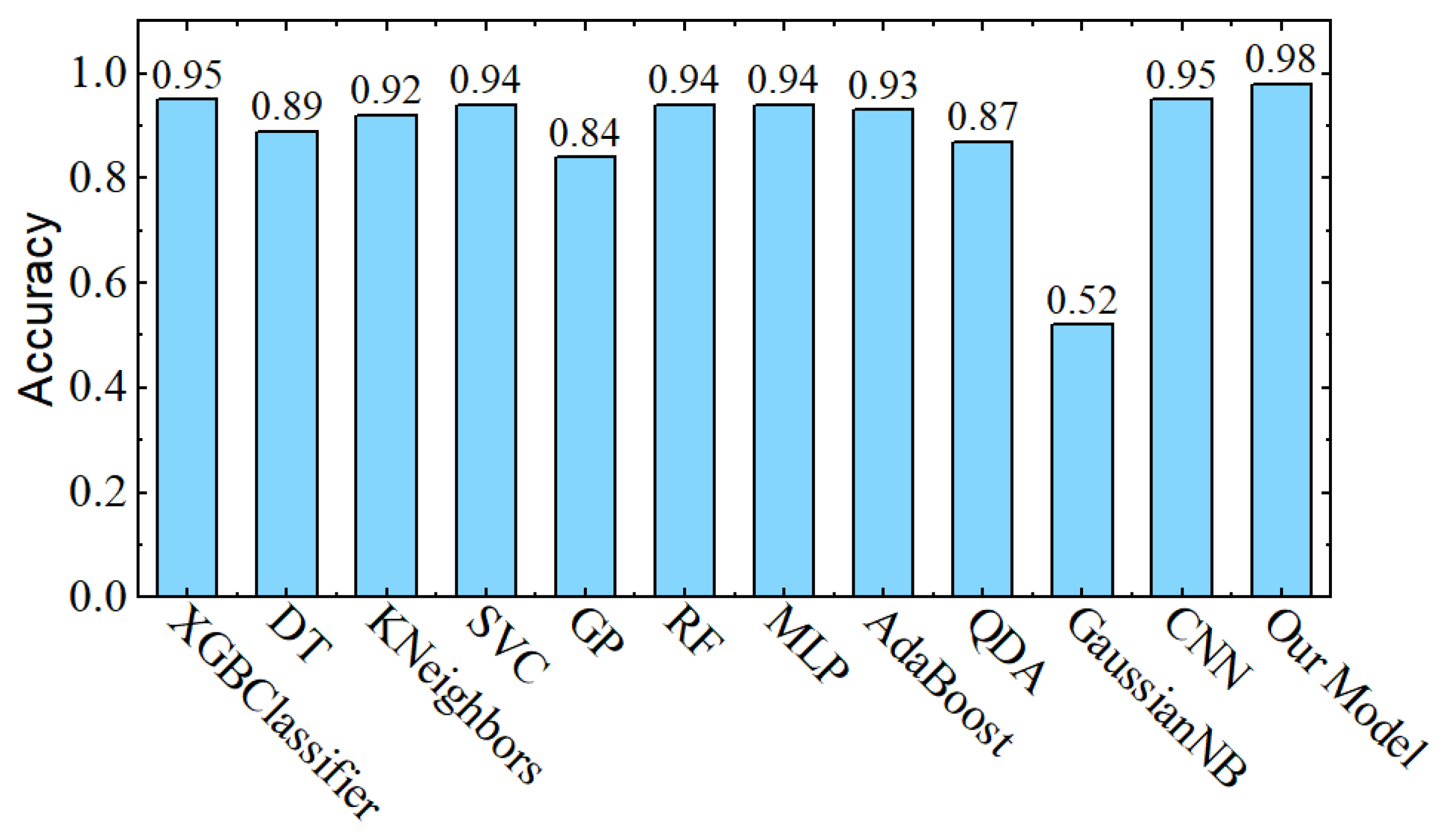
In the last analysis, the impact of bagged ensemble learning is noted. As shown in Figure 1, all selected pre-trained CNN models along with proposed 1D CNN models are arranged in a parallel way, so that properties of these models can be utilized at the same time. These models are used to classify the same data at the same time using the SVM classifier, and then a majority polling is performed to get the final output. As shown in Figure 12, the individual CNN models provide accuracy between 87% and 95%. However, after the bagged ensemble learning arrangement, our final model accuracy has gained a 3% boost. This boost in accuracy has also decreased the BSL to 1.3% (see Figure 13).
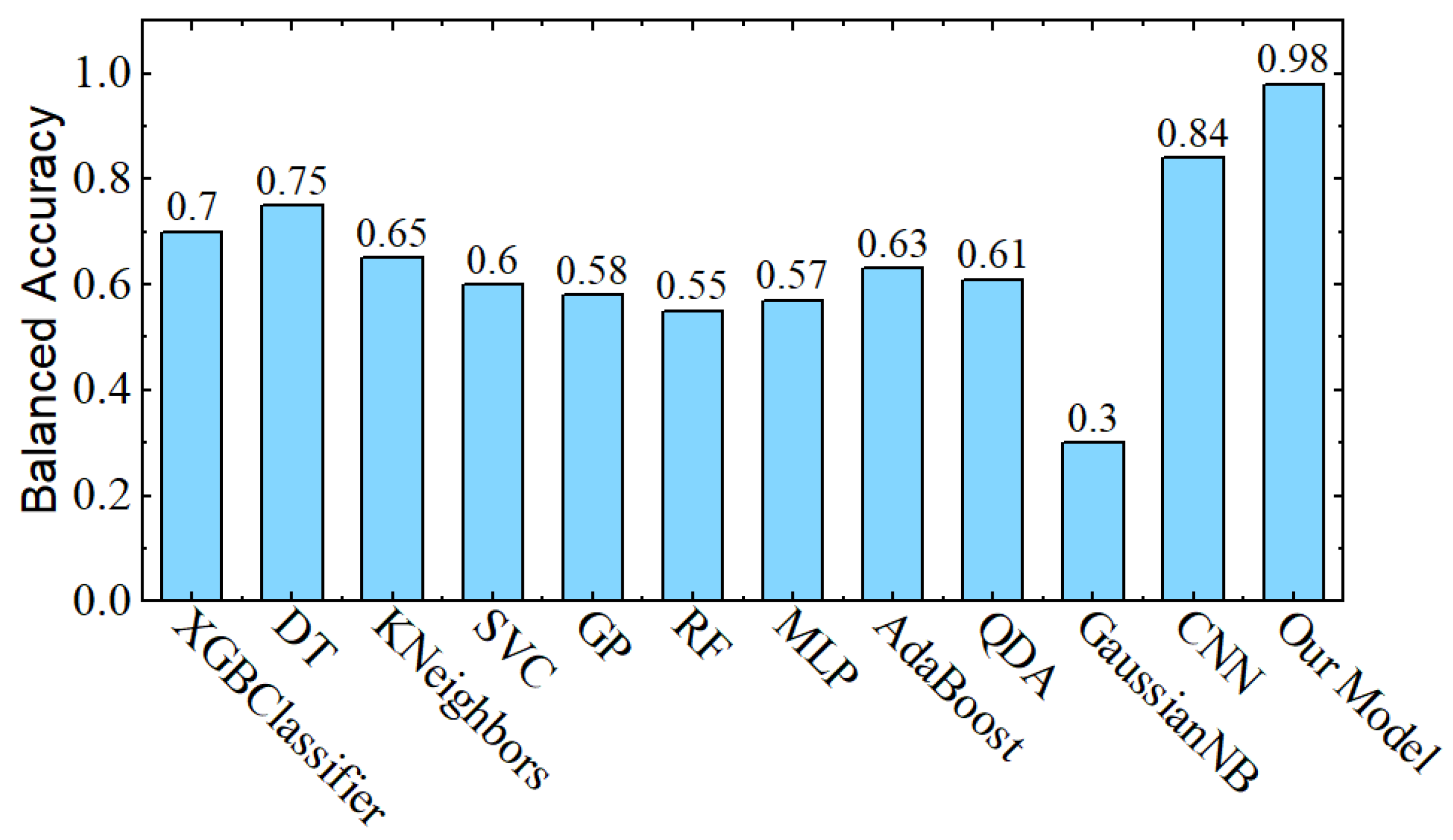
In comparison with the results of the previous sections, Figure 14 shows that the final proposed model out-performed the other paradigms in terms of accuracy and gained a considerable boost in balanced accuracy Figure 15.
To furthermore test the performance of our final model, different performance ratios are calculated. Figure 16 shows the confusion matrix of the bagged ensemble learning based model, we can see that the true positive rate is at 98.5% and the true negative rate at 98.7%.
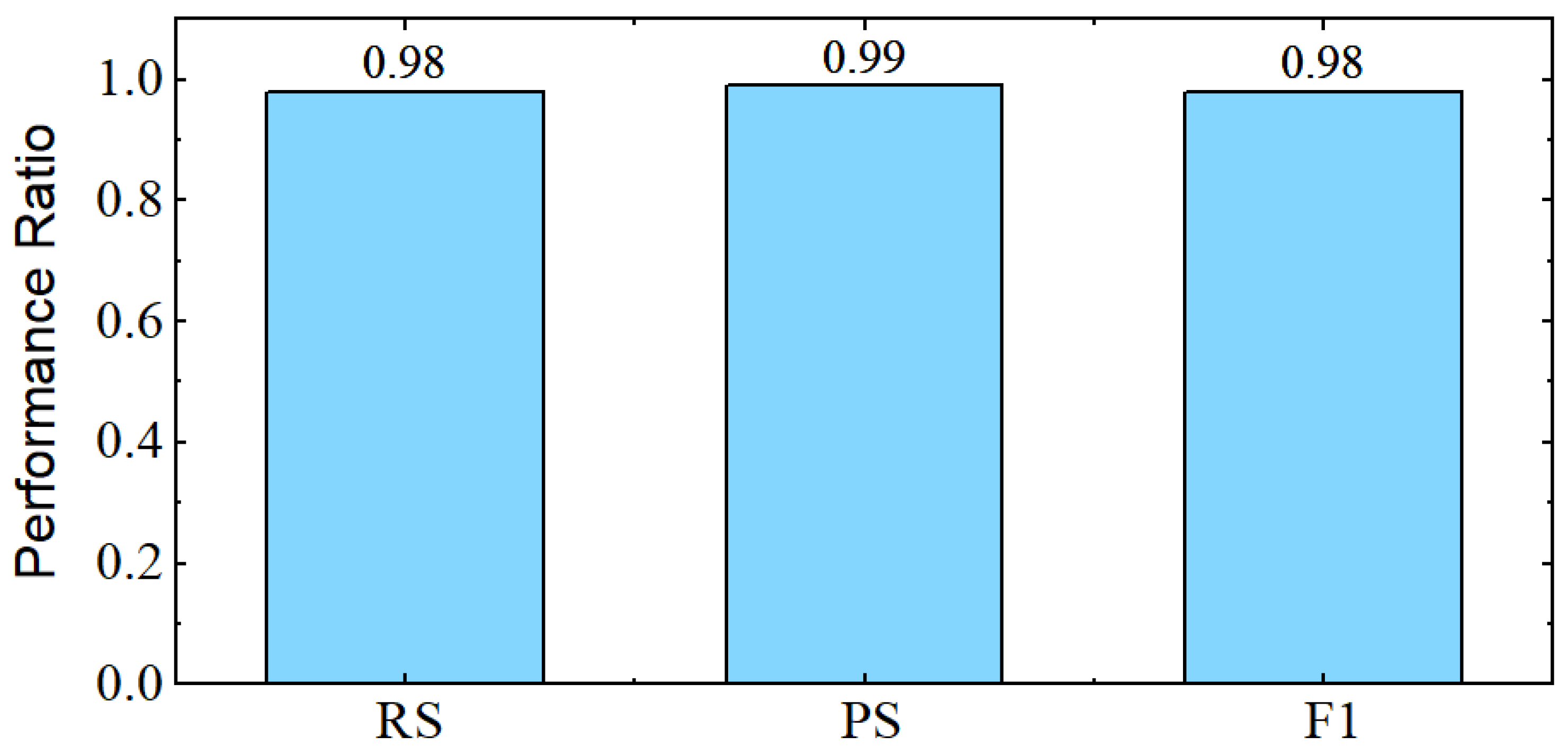
Recal, precision and F1 score are shown in Figure 17. These results show that lining up different models, trained at different samples can increase the performance and also reduces the overall loss of the model.
5. Conclusions
In this work, a bagged ensemble learning-based model is proposed to recognize frauds in auto insurance claims. Three pre-trained CNN models are selected at first, which are minimized by reducing the redundant blocks of layers, and then tweaked to work on 1D data. Along with these pre-trained models, a lightweight CNN model is proposed, consisting of only 19 layers to efficiently work on 1D data. The selected dataset is randomly split into training, validation, and testing portions, so that each CNN model is trained on different data. At the end all CNN models are stacked in parallel, so that the properties of each model can be utilized at the same time. Once a decision is made by each model through the SVM classifier, a majority pooling approach is used to obtain a combined output. The proposed method is tested on publicly available real-word dataset and achieved promising results. The experiments show that used approach boosted the accuracy of the proposed individual 1D CNN, achieving an accuracy of 98% and a low Brier Score Loss of 2%. Due to the imbalanced nature of the dataset, other metrics were also used, namely, balanced accuracy and F1 score. the proposed approach achieves a score of 98% on both metrics, showing the model’s ability to both detect fraudulent and legitimate claims and be accurate with the captured cases.
The outcomes of our investigation show how successful the suggested approach is at spotting false insurance claims. Our approach dealt with an unbalanced dataset and still managed to attain a high level of accuracy. Additionally, the model can learn sophisticated data representations and strengthen its robustness thanks to the usage of CNNs and a bagged ensemble learning method. This study demonstrates the value of applying ensemble learning techniques to the detection of fraudulent insurance claims and opens up possibilities for future study.
Finally, for our future research work, we will investigate how to employ the federated learning approach in order to increase efficiency. In addition, a novel data augmentation approach can also be employed to decrease the impact of imbalanced data. Other pre-trained CNN models can also be employed to increase the performance of the proposed model.
Author Contributions
Conceptualization, Y.A.; Methodology, Y.A.; Validation, M.L.; Writing—original draft, Y.A.; Writing—review and editing, M.L.; Supervision, M.L. and A.A.; Project administration, A.A. All authors have read and agreed to the published version of the manuscript.
Funding
This research received no external funding.
Institutional Review Board Statement
Not applicable.
Informed Consent Statement
Not applicable.
Data Availability Statement
The dataset is accessible under CC0: Public Domain license, and can be downloaded on Kaggle at: https://www.kaggle.com/datasets/shivamb/vehicle-claim-fraud-detection (accessed on 1 November 2022).
Conflicts of Interest
The authors declare no conflict of interest.
References
- Wang, J.H.; Liao, Y.L.; Tsai, T.M.; Hung, G. Technology-based financial frauds in Taiwan: Issues and approaches. In Proceedings of the 2006 IEEE International Conference on Systems, Man and Cybernetics, Taipei, Taiwan, 8–11 October 2006; pp. 1120–1124. [Google Scholar]
- Supraja, K.; Saritha, S. Robust fuzzy rule based technique to detect frauds in vehicle insurance. In Proceedings of the 2017 International Conference on Energy, Communication, Data Analytics and Soft Computing (ICECDS), Chennai, India, 1–2 August 2017; pp. 3734–3739. [Google Scholar]
- Subudhi, S.; Panigrahi, S. Use of optimized Fuzzy C-Means clustering and supervised classifiers for automobile insurance fraud detection. J. King Saud-Univ.-Comput. Inf. Sci. 2020, 32, 568–575. [Google Scholar] [CrossRef]
- Itri, B.; Mohamed, Y.; Mohammed, Q.; Omar, B. Performance comparative study of machine learning algorithms for automobile insurance fraud detection. In Proceedings of the 2019 Third International Conference on Intelligent Computing in Data Sciences (ICDS), Marrakech, Morocco, 28–30 October 2019; IEEE: Piscataway, NJ, USA, 2019; pp. 1–4. [Google Scholar]
- Ngai, E.W.; Hu, Y.; Wong, Y.H.; Chen, Y.; Sun, X. The application of data mining techniques in financial fraud detection: A classification framework and an academic review of literature. Decis. Support Syst. 2011, 50, 559–569. [Google Scholar] [CrossRef]
- Šubelj, L.; Furlan, Š.; Bajec, M. An expert system for detecting automobile insurance fraud using social network analysis. Expert Syst. Appl. 2011, 38, 1039–1052. [Google Scholar] [CrossRef] [Green Version]
- Ghezzi, S.G. A private network of social control: Insurance investigation units. Soc. Probl. 1983, 30, 521–531. [Google Scholar] [CrossRef] [Green Version]
- Clarke, M. The control of insurance fraud: A comparative view. Br. J. Criminol. 1990, 30, 1–23. [Google Scholar] [CrossRef]
- Caron, L.; Dionne, G. Insurance fraud estimation: More evidence from the Quebec automobile insurance industry. In Automobile Insurance: Road Safety, New Drivers, Risks, Insurance Fraud and Regulation; Springer: Boston, MA, USA, 1999; pp. 175–182. [Google Scholar]
- Viaene, S.; Derrig, R.A.; Baesens, B.; Dedene, G.A. comparison of state-of-the-art classification techniques for expert automobile insurance claim fraud detection. J. Risk Insur. 2002, 69, 373–421. [Google Scholar] [CrossRef]
- Phua, C.; Alahakoon, D.; Lee, V. Minority report in fraud detection: Classification of skewed data. ACM Sigkdd Explor. Newsl. 2004, 6, 50–59. [Google Scholar] [CrossRef]
- Šubelj, L.; Bajec, M. Robust network community detection using balanced propagation. Eur. Phys. J. B 2011, 81, 353–362. [Google Scholar] [CrossRef] [Green Version]
- Xu, W.; Wang, S.; Zhang, D.; Yang, B. Random rough subspace based neural network ensemble for insurance fraud detection. In Proceedings of the 4th International Joint Conference on Computational Sciences and Optimization, Kunming, China, 15–19 April 2011; pp. 1276–1280. [Google Scholar]
- Tao, H.; Liu, Z.; Song, X. Insurance fraud identification research based on fuzzy Support Vector Machine with dual membership. In Proceedings of the 2012 International Conference on Information Management, Innovation Management and Industrial Engineering, Sanya, China, 20–21 October 2012; pp. 457–460. [Google Scholar]
- Sundarkumar, G.G.; Ravi, V. A novel hybrid undersampling method for mining imbalanced datasets in banking and insurance. Eng. Appl. Artif. Intell. 2015, 37, 368–377. [Google Scholar] [CrossRef]
- Lee, Y.J.; Yeh, Y.R.; Wang, Y.C.F. Anomaly detection via online oversampling principal component analysis. IEEE Trans. Knowl. Data Eng. 2012, 25, 1460–1470. [Google Scholar] [CrossRef]
- Fu, K.; Cheng, D.; Tu, Y.; Zhang, L. Credit card fraud detection using convolutional neural networks. In Proceedings of the International Conference on Neural Information Processing, Kyoto, Japan, 16–21 October 2016; pp. 483–490. [Google Scholar]
- Zhang, Z.; Zhou, X.; Zhang, X.; Wang, L.; Wang, P. A model based on convolutional neural network for online transaction fraud detection. Secur. Commun. Netw. 2018. [Google Scholar] [CrossRef] [Green Version]
- Xia, H.; Zhou, Y.; Zhang, Z. Auto insurance fraud identification based on a CNN-LSTM fusion deep learning model. Int. J. Ad Hoc Ubiquitous Comput. 2022, 39, 37–45. [Google Scholar] [CrossRef]
- Rawat, W.; Wang, Z. Deep convolutional neural networks for image classification: A comprehensive review. Neural Comput. 2017, 29, 2352–2449. [Google Scholar] [CrossRef]
- Dhillon, A.; Verma, G.K. Convolutional neural network: A review of models, methodologies and applications to object detection. Prog. Artif. Intell. 2020, 9, 85–112. [Google Scholar] [CrossRef]
- Abdullah, S.M.S.; Abdulazeez, A.M. Facial expression recognition based on deep learning convolution neural network: A review. J. Soft Comput. Data Min. 2008, 2, 53–65. [Google Scholar]
- Anwar, S.M.; Majid, M.; Qayyum, A.; Awais, M.; Alnowami, M.; Khan, M.K. Medical image analysis using convolutional neural networks: A review. J. Med Syst. 2018, 42, 1–13. [Google Scholar] [CrossRef] [Green Version]
- Tian, X.; Han, H. Deep convolutional neural networks with transfer learning for automobile damage image classification. J. Database Manag. (JDM) 2022, 33, 1–16. [Google Scholar] [CrossRef]
- Szegedy, C.; Liu, W.; Jia, Y.; Sermanet, P.; Reed, S.; Anguelov, D.; Erhan, D.; Vanhoucke, V.; Rabinovich, A. Going deeper with convolutions. In Proceedings of the IEEE Conference on Computer Vision and Pattern Recognition, Boston, MA, USA, 7–12 June 2015; pp. 1–9. [Google Scholar]
- Dong, N.; Zhao, L.; Wu, C.H.; Chang, J.F. Inception v3 based cervical cell classification combined with artificially extracted features. Appl. Soft Comput. 2020, 93, 106311. [Google Scholar] [CrossRef]
- Wang, C.; Chen, D.; Hao, L.; Liu, X.; Zeng, Y.; Chen, J.; Zhang, G. Pulmonary image classification based on inception-v3 transfer learning model. IEEE Access 2019, 7, 146533–146541. [Google Scholar] [CrossRef]
- Xia, X.; Xu, C.; Nan, B. Inception-v3 for flower classification. In Proceedings of the 2017 2nd International Conference on Image, Vision and COMPUTING (ICIVC), Chengdu, China, 2–4 June 2017; pp. 783–787. [Google Scholar]
- Matoušek, J.; Tihelka, D. A comparison of convolutional neural networks for glottal closure instant detection from raw speech. In Proceedings of the ICASSP 2021—2021 IEEE International Conference on Acoustics, Speech and Signal Processing (ICASSP), Toronto, ON, Canada, 6–11 June 2021; pp. 6938–6942. [Google Scholar]
- He, K.; Zhang, X.; Ren, S.; Sun, J. Deep residual learning for image recognition. In Proceedings of the IEEE Conference on Computer Vision and Pattern Recognition, Las Vegas, NV, USA, 27–30 June 2016; pp. 770–778. [Google Scholar]
- Microsoft/Resnet-101 · Hugging Face. Available online: https://huggingface.co/microsoft/resnet-101 (accessed on 18 January 2023).
- Ghosal, P.; Nandanwar, L.; Kanchan, S.; Bhadra, A.; Chakraborty, J.; Nandi, D. Brain tumor classification using ResNet-101 based squeeze and excitation deep neural network. In Proceedings of the 2019 Second International Conference on Advanced Computational and Communication Paradigms (ICACCP), Majitar, India, 25–28 February 2019; pp. 1–6. [Google Scholar]
- Demir, A.; Yilmaz, F.; Kose, O. Early detection of skin cancer using deep learning architectures: Resnet-101 and inception-v3. In Proceedings of the 2019 Medical Technologies Congress (TIPTEKNO), Izmir, Turkey, 3–5 October 2019; pp. 1–4. [Google Scholar]
- LSVRC 2012 Results, image-net.org. Available online: https://image-net.org/challenges/LSVRC/2012/results.html (accessed on 18 January 2023).
- Krizhevsky, A.; Sutskever, I.; Hinton, G.E. Imagenet classification with deep convolutional neural networks. Commun. ACM 2017, 60, 84–90. [Google Scholar] [CrossRef] [Green Version]
- Hancock, J.; Khoshgoftaar, T.M. Performance of catboost and xgboost in medicare fraud detection. In Proceedings of the 2020 19th IEEE International Conference on Machine Learning and Applications (ICMLA), Miami, FL, USA, 14–17 December 2020; pp. 572–579. [Google Scholar]
- Zhang, Y.; Tong, J.; Wang, Z.; Gao, F. Customer transaction fraud detection using xgboost model. In Proceedings of the 2020 International Conference on Computer Engineering and Application (ICCEA), Guangzhou, China, 18–20 March 2020; pp. 554–558. [Google Scholar]
- Hassan, A.K.I.; Abraham, A. Modeling insurance fraud detection using imbalanced data classification. In Advances in Nature and Biologically Inspired Computing; Springer: Cham, Switzerland, 2016; pp. 117–127. [Google Scholar]
- Awoyemi, J.O.; Adetunmbi, A.O.; Oluwadare, S.A. Credit card fraud detection using machine learning techniques: A comparative analysis. In Proceedings of the International Conference on Computing Networking and Informatics (ICCNI), Ota, Nigeria, 29–31 October 2017; pp. 1–9. [Google Scholar]
- Al-Hashedi, K.G.; Magalingam, P. Financial fraud detection applying data mining techniques: A comprehensive review from 2009 to 2019. Comput. Sci. Rev. 2021, 40, 100402. [Google Scholar] [CrossRef]
- Fan, J.; Zhang, Q.; Zhu, J.; Zhang, M.; Yang, Z.; Cao, H. Robust deep auto-encoding Gaussian process regression for unsupervised anomaly detection. Neurocomputing 2020, 376, 180–190. [Google Scholar] [CrossRef]
- Li, Y.; Yan, C.; Liu, W.; Li, M. Research and application of Random Forest model in mining automobile insurance fraud. In Proceedings of the 2016 12th International Conference on Natural Computation, Fuzzy Systems and Knowledge Discovery (ICNC-FSKD), Changsha, China, 13–15 August 2016; pp. 1756–1761. [Google Scholar]
- Freund, Y.; Schapire, R.E. A decision-theoretic generalization of on-line learning and an application to boosting. J. Comput. Syst. Sci. 1997, 55, 119–139. [Google Scholar] [CrossRef] [Green Version]
- Randhawa, K.; Loo, C.K.; Seera, M.; Lim, C.P.; Nandi, A.K. Credit card fraud detection using adaboost and majority voting. IEEE Access 2018, 6, 14277–14284. [Google Scholar] [CrossRef]
- Fraud Stats, InsuranceFraud.org. 2022. Available online: https://insurancefraud.org/fraud-stats/ (accessed on 18 January 2023).
Figure 1.
Architecture of the proposed Bagged Ensemble Learning Model.

Figure 2.
Association between Age and Fraud Found. The y axis “FraudFound_P” represents the number of rows for FraudFound_P = 1.
Figure 2.
Association between Age and Fraud Found. The y axis “FraudFound_P” represents the number of rows for FraudFound_P = 1.

Figure 3.
Association between Age and No Fraud Found. The y axis “FraudFound_P” represents the number of rows for FraudFound_P = 0.
Figure 3.
Association between Age and No Fraud Found. The y axis “FraudFound_P” represents the number of rows for FraudFound_P = 0.

Figure 4.
Class distribution of fraud in the selected dataset. The x axis represents the two classes of No Fraud Found (FraudFound_P = 0) and Fraud Found (FraudFound_P = 1). The FraudFound class represents 6.36% of the total records.
Figure 4.
Class distribution of fraud in the selected dataset. The x axis represents the two classes of No Fraud Found (FraudFound_P = 0) and Fraud Found (FraudFound_P = 1). The FraudFound class represents 6.36% of the total records.

Figure 5.
Driver rating class distribution as per the total observations. N total represents the count of accidents claims for each class, fraudulent or not.
Figure 5.
Driver rating class distribution as per the total observations. N total represents the count of accidents claims for each class, fraudulent or not.

Figure 6.
Accuracy results before and after cleaning and augmentation.

Figure 7.
Balanced Accuracy results before and after cleaning and augmentation.

Figure 8.
BSL results before and after data augmentation.

Figure 9.
Performance ratios of the proposed CNN model, before and after cleaning and augmentation.

Figure 10.
Impact of different epochs on the efficiency of proposed model.

Figure 11.
Impact of the fine tuning on the model. (a,b) show the accuracy and loss evolution during training on the validation set for a fixed epochs of 70 and 0.002 learning rate.
Figure 11.
Impact of the fine tuning on the model. (a,b) show the accuracy and loss evolution during training on the validation set for a fixed epochs of 70 and 0.002 learning rate.

Figure 12.
Results of the individual minimized pre-trained CNNs and the proposed 1D CNN model without the bagged ensemble learning arrangement, in comparison with the final model with the proposed bagged ensemble learning architecture.
Figure 12.
Results of the individual minimized pre-trained CNNs and the proposed 1D CNN model without the bagged ensemble learning arrangement, in comparison with the final model with the proposed bagged ensemble learning architecture.

Figure 13.
Final Brier Score Loss results of the proposed model in comparison with other paradigms.

Figure 14.
Final accuracy results of the proposed model in comparison with other paradigms.

Figure 15.
Final balanced accuracy results of the proposed model in comparison with other paradigms.
Figure 15.
Final balanced accuracy results of the proposed model in comparison with other paradigms.

Figure 16.
Confusion matrix of the proposed Bagged ensemble learning based model.

Figure 17.
Recal, precision and F1 score of our final bagged ensemble learning based model.


Table 1.
Detailed information of proposed 1D CNN model.
| # | Layer | Parameters | Input | Output |
|---|---|---|---|---|
| 1 | Convolution1D_1 | Channels = 32 Kernels = 14 Pooling = 0.32 | 64 × 1 × 32 × 480 | 64 × 32 × 32 × 480 |
| 2 | Batch_Normalization_1 | Channels = 32 | 64 × 32 × 32 × 480 | 64 × 64 × 32 × 480 |
| 3 | Convolution1D_2 | Channels = 64 Kernels = (28,1) Pooling = 0.0 | 64 × 64 × 32 × 480 | 64 × 64 × 1 × 480 |
| 4 | Batch_Normalization_2 | Channels = 64 | 64 × 64 × 1 × 480 | 64 × 64 × 1 × 480 |
| 5 | ReLU_1 | - | 64 × 64 × 1 × 480 | 64 × 64 × 1 × 480 |
| 6 | Max-Pooling_1 | [1,2] | 64 × 64 × 1 × 480 | 64 × 64 × 1 × 228 |
| 7 | Dropout | 0.5 | 64 × 64 × 1 × 228 | 32 × 32 × 1 × 114 |
| 8 | Convolution1D_3 | Channels = 16 Kernels = 7 Pooling = 0.64 | 32 × 32 × 1 × 114 | 64 × 16 × 32 × 114 |
| 9 | Batch_Normalization_3 | Channels = 32 | 64 × 16 × 32 × 114 | 64 × 32 × 32 × 114 |
| 10 | Convolution1D_4 | Channels = 64 Kernels = (28,1) Pooling = 0.0 | 64 × 32 × 32 × 114 | 64 × 32 × 1 × 114 |
| 11 | Batch_Normalization_4 | Channels = 32 | 64 × 32 × 1 × 114 | 64 × 32 × 1 × 114 |
| 12 | ReLU_2 | - | 64 × 32 × 1 × 114 | 64 × 32 × 1 × 114 |
| 13 | Max-Pooling_2 | [1,1] | 64 × 32 × 1 × 114 | 64 × 32 × 1 × 57 |
| 14 | Dropout | 0.5 | 64 × 32 × 1 × 57 | 32 × 16 × 1 × 27 |
| 15 | Fully_Connected_1 | Input = 32 Output = 32 | 32 × 16 × 1 × 27 | 32 × 16 × 32 |
| 16 | ReLU_3 | - | 32 × 16 × 32 | 32 × 16 × 32 |
| 17 | Fully_Connected_2 | Input = 16 Output = 16 | 32 × 16 × 32 | 32 × 16 × 16 |
| 18 | ReLU_4 | - | 32 × 16 × 32 | 32 × 16 × 32 |
| 19 | Label Output | - | - | - |
Table 2.
Impact of different split ratio on the efficiency of proposed model.
| Split Ratio | Accuracy |
|---|---|
| 40–30–30 | 0.87 |
| 50–25–25 | 0.90 |
| 60–20–20 | 0.93 |
| 70–15–15 | 0.95 |
| 80–10–10 | 0.94 |
| 90–5–5 | 0.94 |
Table 3.
Impact of different Learning rates on the efficiency of proposed model.
| Initial Learning Rate | Accuracy |
|---|---|
| 0.01 | 0.78 |
| 0.02 | 0.87 |
| 0.001 | 0.92 |
| 0.002 | 0.95 |
| 0.0001 | 0.92 |
| 0.0002 | 0.86 |
Table 4.
Results of pre-trained model while using full and partial architectures.
| Model | AlexNet | Inception-V3 | Resnet-101 | |||
|---|---|---|---|---|---|---|
| Selected Blocks | Acc | Selected Blocks | Acc | Selected Blocks | Acc | |
| Original | -all- | 0.83 | -all- | 0.84 | -all- | 0.87 |
| Minimized | 1 | 0.81 | 1 | 0.8 | 1 | 0.74 |
| 2 | 0.87 | 2 | 0.83 | 2 | 0.81 | |
| - | - | 3 | 0.89 | 3 | 0.88 | |
| - | - | 4 | 0.85 | 4 | 0.91 | |
| - | - | 5 | 0.82 | 5 | 0.86 | |
| - | - | 6 | 0.83 | 6 | 0.85 | |
Disclaimer/Publisher’s Note: The statements, opinions and data contained in all publications are solely those of the individual author(s) and contributor(s) and not of MDPI and/or the editor(s). MDPI and/or the editor(s) disclaim responsibility for any injury to people or property resulting from any ideas, methods, instructions or products referred to in the content. |
© 2023 by the authors. Licensee MDPI, Basel, Switzerland. This article is an open access article distributed under the terms and conditions of the Creative Commons Attribution (CC BY) license (https://creativecommons.org/licenses/by/4.0/).
Share and Cite
MDPI and ACS Style
Abakarim, Y.; Lahby, M.; Attioui, A. A Bagged Ensemble Convolutional Neural Networks Approach to Recognize Insurance Claim Frauds. Appl. Syst. Innov. 2023, 6, 20. https://doi.org/10.3390/asi6010020
AMA Style
Abakarim Y, Lahby M, Attioui A. A Bagged Ensemble Convolutional Neural Networks Approach to Recognize Insurance Claim Frauds. Applied System Innovation. 2023; 6(1):20. https://doi.org/10.3390/asi6010020
Chicago/Turabian StyleAbakarim, Youness, Mohamed Lahby, and Abdelbaki Attioui. 2023. "A Bagged Ensemble Convolutional Neural Networks Approach to Recognize Insurance Claim Frauds" Applied System Innovation 6, no. 1: 20. https://doi.org/10.3390/asi6010020