
A Water Tank Level Control System with Time Lag Using CGSA and Nonlinear Switch Decoration


Navigation College, Dalian Maritime University, Dalian 116026, China
*
Authors to whom correspondence should be addressed.
Appl. Syst. Innov. 2023, 6(1), 12; https://doi.org/10.3390/asi6010012
Submission received: 10 December 2022
/
Revised: 31 December 2022
/
Accepted: 3 January 2023
/
Published: 16 January 2023
(This article belongs to the Section Control and Systems Engineering)
Abstract
:Tank level control has some unavoidable factors such as disturbance, non-linearity, and time lag. This paper proposes a simple and robust control scheme with nice energy-saving effects and smooth output to improve the quality of the controller and meet real-world application requirements. A linear controller is first designed using a third-order closed-loop gain-shaping algorithm. We then use an arcsine function to modify the system with non-linear switching to reduce the effect of the non-linear modification on the dynamic performance of the control system. Furthermore, we use the Nyquist stability criterion to demonstrate the stability of the closed-loop system in the presence of time lag. The results of the final simulation experiment show that the controller not only has high control quality but also has the characteristics of energy saving and smooth output under the condition of lag and pump performance constraints. These features are necessary for extending the life of the pump and enhancing the applicability of the tank level controller.
1. Introduction
Level control is commonly applied in large industrial automation production. In the shipping industry, the level control of various ship compartments plays a vital role in coordinating the safe navigation of ships, such as oil tanks, ballast tanks, and freshwater tanks. However, tank-level control systems are often subject to uncertainties such as time-varying state, non-linearity, and time lag. So many scholars have conducted a lot of research on this problem. Li et al. [1] and Zhang et al. [2] designed the water tank level controller based on the PID method, the simulation experiments showed that the PID controller has a better control performance. However, there is still the problem of complex parameter rectification to some extent. Thus, the idea of fuzzy logic and PID control worked together to solve the problem of parameter tuning [3,4]. Olivas et al. [5] used the ant colony algorithm (ACO) to further optimize the fuzzy controller for the water tank. However, this type of intelligent algorithm is more complex and computationally intensive. Young et al. [6] proposed a sliding mode control theory. It is widely used in applications due to its robustness and simplicity. The water tank level controller designed based on the sliding mode control theory [7,8,9,10] worked well. However, the discontinuous switching characteristics of the variable structure can cause jitter and vibration in the system. It reduces the service life of the pump and is not conducive to practical engineering applications. Therefore, it is necessary to design a simple tank level control system with the following characteristics. (1) Clear engineering implications and low calculation load. (2) Under the constraints of pump performance constraints, external environmental interference, and time lag, the controller should reduce energy loss and extend the service life of the pump while ensuring high control effects.
So, we use a closed-loop gain-shaping algorithm (CGSA) to design the controller. The algorithm is simplified as an engineering application of robust control and has the advantages of a simple design process and obvious physical significance. Zhang et al. [11] proposed a new control scheme for industrial multiple-input multiple-output (MIMO) systems with a time lag using the CGSA method. Guan et al. [12] used CGSA to design a robust PID fin control system to achieve ship rocking reduction control. Jiang et al. [13] designed a wireless network control system based on CGSA and verified its role in a ship course keeping control through a simulation platform. The non-linear modification technique adds a non-linear function component between the control input and the system model. It is often combined with CGSA algorithms to solve the issue of high energy consumption. The technique is widely used in various fields such as ship heading control [14,15,16,17], track keeping [18,19,20], pressure control in insulated spaces [21], parameter identification of ship response models [22], tank level control [23,24,25,26], etc. However, for tank level control, CGSA was modified by different functions, such as the arctan [23], sinusoidal function [24], and S function [25]. The control system was modified by the Gaussian function and applied to the control of liquid tanks of LNG vessels [26]. The above research results were searching for the effect of different nonlinear functions on the modification of the CGSA algorithm and applying them to different fields. In this paper, we propose a nonlinear switching theory to reduce its impact on the dynamic performance of the controller while ensuring the original decoration effect. Moreover, we introduce new evaluation metrics to analyze the effectiveness of the control system. The main contributions are listed by
(1) We design a concise linear controller using a third-order closed-loop gain-shaping algorithm and modify the linear control law by a nonlinear switching modification technique based on the arcsine function. Meanwhile, a pure time lag component of 0.8 s is introduced to fit the realistic situation, and finally, we use the Nyquist stability criterion to demonstrate the stability of the control system.
(2) When doing simulation experiments, we consider the performance constraints of the pump and little interference. Then, we introduce a new evaluation index system to analyze comparatively the controller. The experimental results show that this controller has significant advantages in terms of energy saving, safety, and smoothing.
The remainder of the paper is organized as follows: In Section 2, we simplify the non-linear tank level model. In Section 3, the control system is designed. In Section 4, we perform stability analysis in the presence of time lag. In Section 5, We provide simulation examples, and Section 6 concludes.
2. Tank Level Model
Assumption. An idealized single tank exists, where both input and output regulating valves are in action to achieve the set height. The key mathematical notations used in this model are listed in Table 1.
The difference between the inflow and outflow is
where is the tank liquid storage volume.
where is the valve flow coefficient.
where is the cross-sectional area of the output tube.
Equation (3) can be converted to linear at the equilibrium point , then the liquid resistance R can be expressed as
Substituting Equations (2) and (4) into Equation (1) and converting them into transfer function form, we receive
where, . The linear model (5) is used for the design of the controller, while the non-linear model (1) (3) is used for system simulation to verify the robustness of the designed controller. Assuming that the height of the tank used for this paper is 2 m, the cross-sectional area of the tank is , the cross-sectional area of the output pipe is , the initial level is 0.5 m, and the maximum inlet volume of the tank is , then , , , [22].
However, the simplified model responds nearly 40% faster than the actual situation [27]. To improve the simulation accuracy of the linear tank control system, a first-order inertial system was added to Equation (5), and it was verified that the regulation time was similar to the actual situation in [27]. Thus, this paper uses this model to improve the confidence of the system simulation, and the new model transfer function is
3. Control System Structure Design
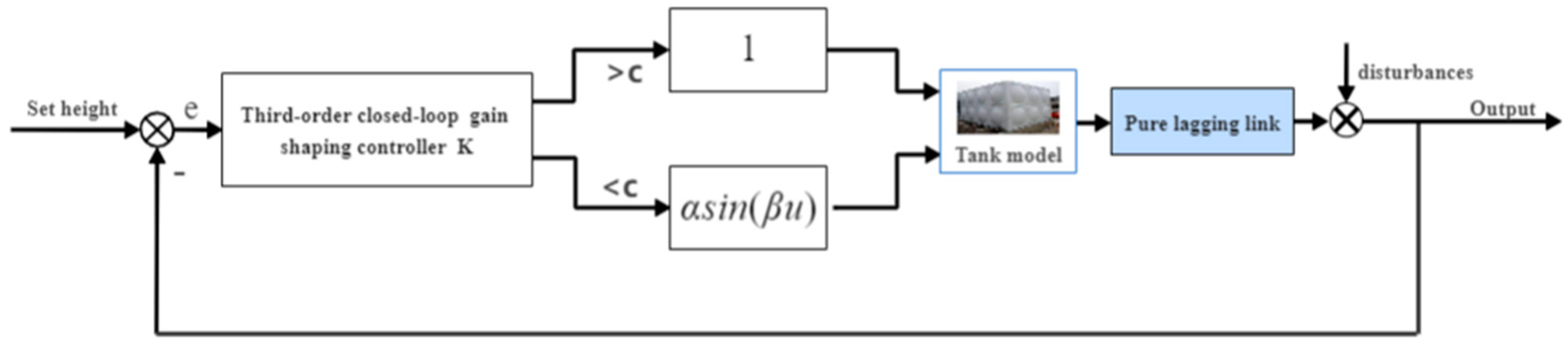
In this section, we first design the controller using the CGSA and then modify the above-level-control system using an arcsine function. We add a pure time lag component after the level model to fit the actual situation. The control system structure is shown in Figure 1.
3.1. Introduction of the Closed-Loop Gain Shaping Algorithm
The closed-loop gain-shaping algorithm is a proposed simple and robust control method for stable MIMO processes based on robust control theory. The core of the method is to determine the final expression of the closed-loop transfer function matrix of the system and to design the robust controller using the main parameters of the closed-loop system, i.e., the maximum singular value, bandwidth of frequency, high frequency asymptote slope, and spectrum peak of the closed-loop.
A control algorithm based on closed-loop gain-shaping is given by observing the mixed sensitivity singular value curve of control S/T (see Figure 2) and the correlation between the sensitivity function S(, G is the controlled object and is the controller) and the complementary sensitivity function T(). According to the four engineering parameters of the maximum singular value, the bandwidth of frequency, the high frequency asymptote slope, and the spectrum peak of the closed-loop, the result of the hybrid sensitivity control algorithm using control is used to construct the complementary sensitivity function T. The correlation between T and the sensitivity function T is applied to indirectly construct the sensitivity function T, and finally, the controller K is inverted.
3.2. Controller Design
We use the third-order CGSA to design the tank level controller and set the bandwidth frequency of the closed-loop system to . Then the complementary sensitivity function of the tank level control system at this time is also the closed-loop transfer function of the system.
By substituting Equation (6) into Equation (7), the final robust controller is obtained as
As can be seen from Equation (8), the controller designed using the third-order closed-loop gain-shaping algorithm is in the form of a typical PD controller with an oscillating component in series. It is simple and easy to implement, solving the problem of complex parameterization and the unclear physical meaning of conventional PD controllers.
3.3. Improved Non-Linear Switch Modification
The non-linear modifier switching technique is essentially a segmentation function. In this paper, the segmentation function is constructed using the arcsine function in the following form.
where and .
It indicates that the system output differs significantly from the set output when u is large. It is often the initial stage of the control process or a situation where a major disturbance occurs. At this time, the arcsine non-linear modification does not work, maintaining the dynamic performance of the control law (8). It means that the difference between the system output and the set output is little when u is small. It is often the stable phase of the control process or a situation where small disturbances occur. Now the arcsine non-linear modification takes effect, making the control input smaller with little impact on the dynamic performance of the control law (8) and thus reducing energy consumption. Since the dynamic performance of the control law (8) remains unchanged for . So, we list the following analysis for the case where .
When , we choose to retain the first-order Taylor expansion of the arcsine function.
(1) Effect on the steady state of the system
Assume that the input is a unit step signal and then analyze the output steady-state values using a modified model of the control object. According to the final value theorem of the Rasch transform, we obtain Equation (11).
Therefore, the non-linear switching modification of the arcsine function does not affect the final steady state of the system.
(2) Effect on the dynamic performance
Equation (12) is the transfer function of the closed-loop system. According to the closed-loop gain-shaping theory, the open-loop transfer function GK of the system meets the requirements of high gain at low frequencies and low gain at high frequencies when . Therefore, in the low-frequency range of Equation (12) compared with the standard feedback system , adding has little effect on the dynamic performance of the system.
(3) Effect on controller output
Equation (13) is the transfer function from the input to the controller output. The numerator of Equation (13) decreases more significantly than the denominator. So will reduce the control output. Non-linear switching technology is the introduction of to reduce energy consumption during the stabilization phase of the control, but at the same time to reduce the output.
4. Stability Analysis
In this section, we begin with an individual analysis of the control law (8) to explore its inherent stability performance. Afterward, the control system, which has the addition of non-linear switching modifications and time lag, is proved to be stable.
The stability analysis of a tank level feedback controller designed based on a closed-loop gain-shaping algorithm is commonly used in the Lyapunov stability theory [22,23,24]. In this paper, the controller follows this scheme and finds that it is necessary to construct and solve a positive definite real symmetric matrix, which is computationally more complex and abstract. Therefore, we refer to the proof of [19] to analyze the stability of the third-order closed-loop gain-forming controller using the Nyquist stability criterion in the frequency domain approach.
4.1. Improved Non-Linear Switch Modification
Theorem 1.
The closed-loop system of the controller designed using the third-order closed-loop gain-shaping algorithm is stable with amplitude margin and phase angle margin under the condition .
Proof:
The open-loop transfer function of the system is obtained from Equation (8):
Taking into the Equation (14).
Assume that the cut-off frequency is and the phase angle junction frequency is .
The solution is
Further solving for the phase angle margin , amplitude margin .
When , the real part of is
□
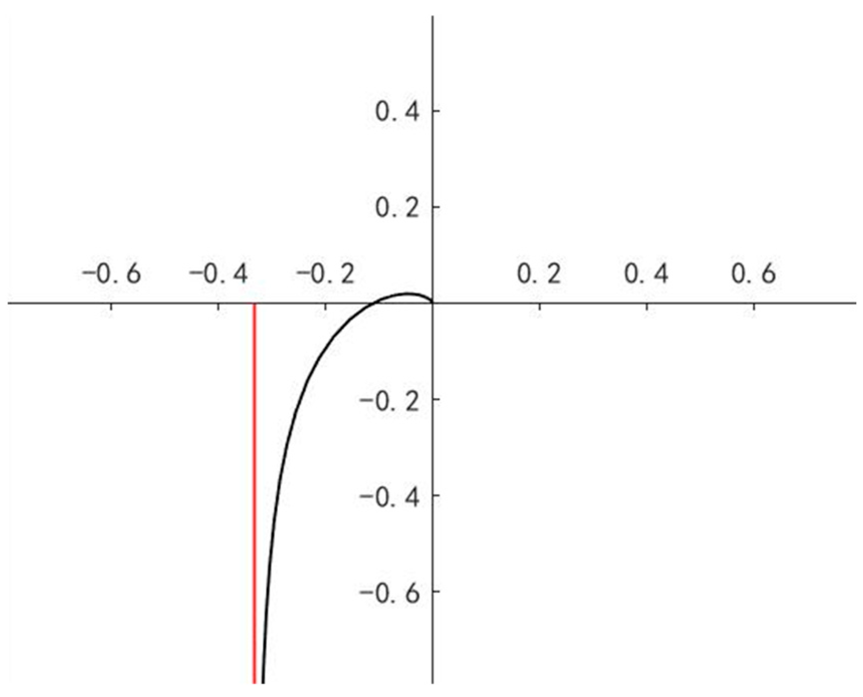
Apparently, . As changes from 0 to infinity, the amplitude and phase angle decreases. When tends to infinity, the phase angle of all three complex vectors is , and the amplitude is infinity. Substituting into Equation (7) we obtain . We make the magnitude-phase characteristic curve of the system as shown in Figure 3.
From the Nyquist stability criterion, we obtain
P is the number of poles in the right half-plane of the open-loop transfer function. N is the number of turns of the Nyquist curve enclosing and Z is the number of poles in the right half-plane of the closed-loop transfer function. In summary, this closed-loop system is stable. Its phase angle margin and amplitude margin .
4.2. Control System Stability Analysis
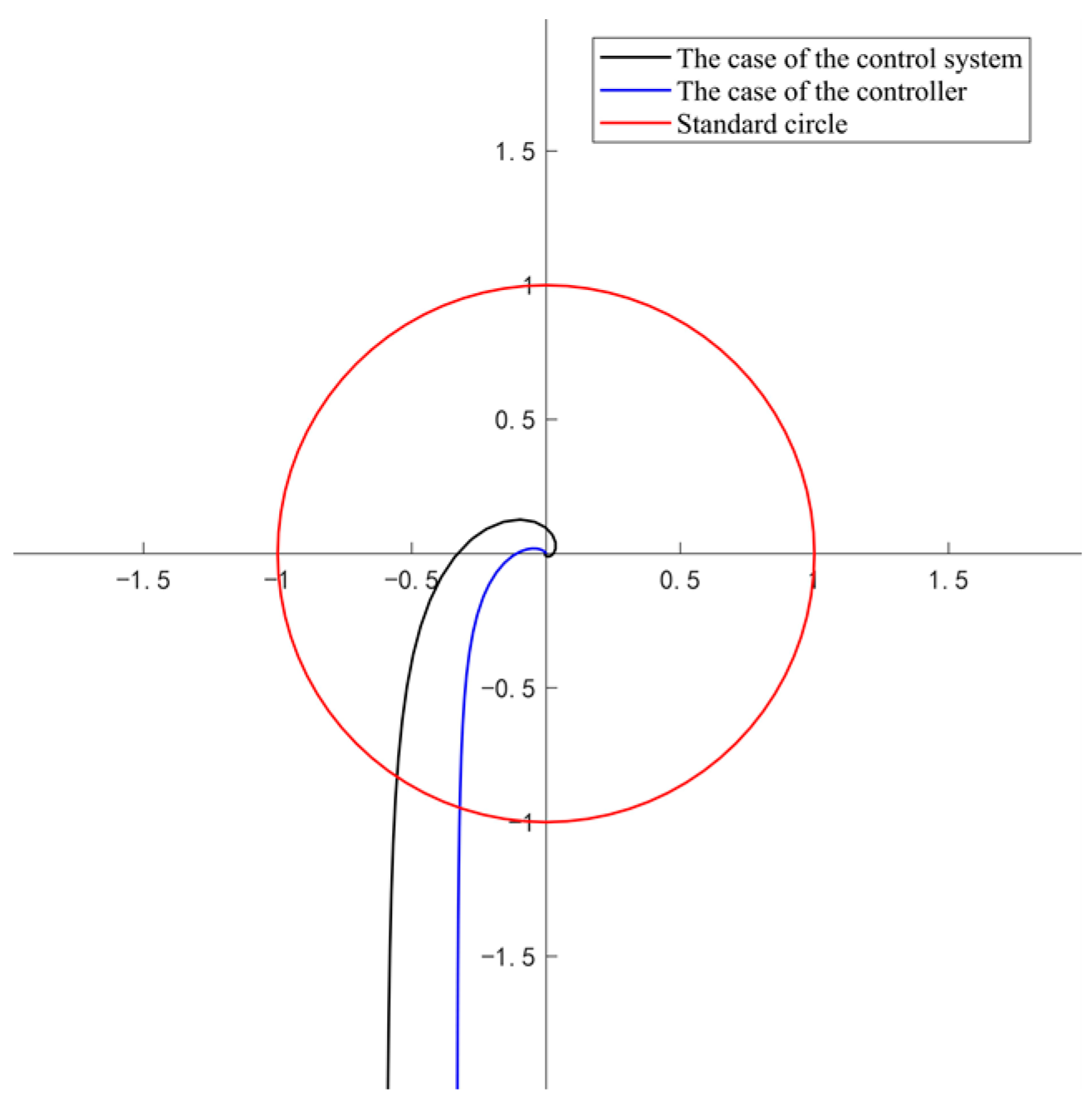
We add a pure time lag component of 0.8 s to the simulation system to fit the actual situation. However, this results in a degradation of the quality of the control and a reduction in the stability of the system. For this reason, we plot the amplitude-phase characteristic curve for the combined effect of the non-linear maximum modifier and the 0.8 s pure time lag component as shown in Figure 4 and use the Nyquist stability criterion to determine the stability of the system.
The blue line shows the magnitude-phase characteristic curve of the original system. The black line is the amplitude-phase characteristic curve of the above two links acting together.
As a result, the system remains stable. However, the non-linear switching modification selectively changes the open-loop transfer function gain, affecting the amplitude margin of the system. Additionally, the introduction of a pure time lag component reduces the phase angle junction frequency of the system, thus reducing the phase angle margin.
5. Simulation Experiments
In this section, simulations are used to verify the effectiveness of the proposed controller. The second-order CGSA controller modified by the Gaussian function has good energy efficiency and strong robustness in the literature [26]. We select it as a reference and compare it with the proposed controller.
5.1. Design of Evaluation Indexes
Traditional water tank control systems are evaluated through a comprehensive performance evaluation index [23,24,25,26]. It cannot analyze all aspects of the control system. Moreover, as research progresses, energy efficiency, safety, and economy become new goals to be pursued. For this reason, we introduce the following metrics [19] to evaluate the performance of the controller proposed in this paper in the presence of disturbances and time lag. The MTV is used to determine the degree of variation in pumping speed, which is necessary to study the life of the pump. The MAE is used to measure the response performance of the system output. Additionally, MIA is used to measure the energy consumption of the corresponding control algorithm, see Equations (21)–(23).
5.2. Comparative Experiments
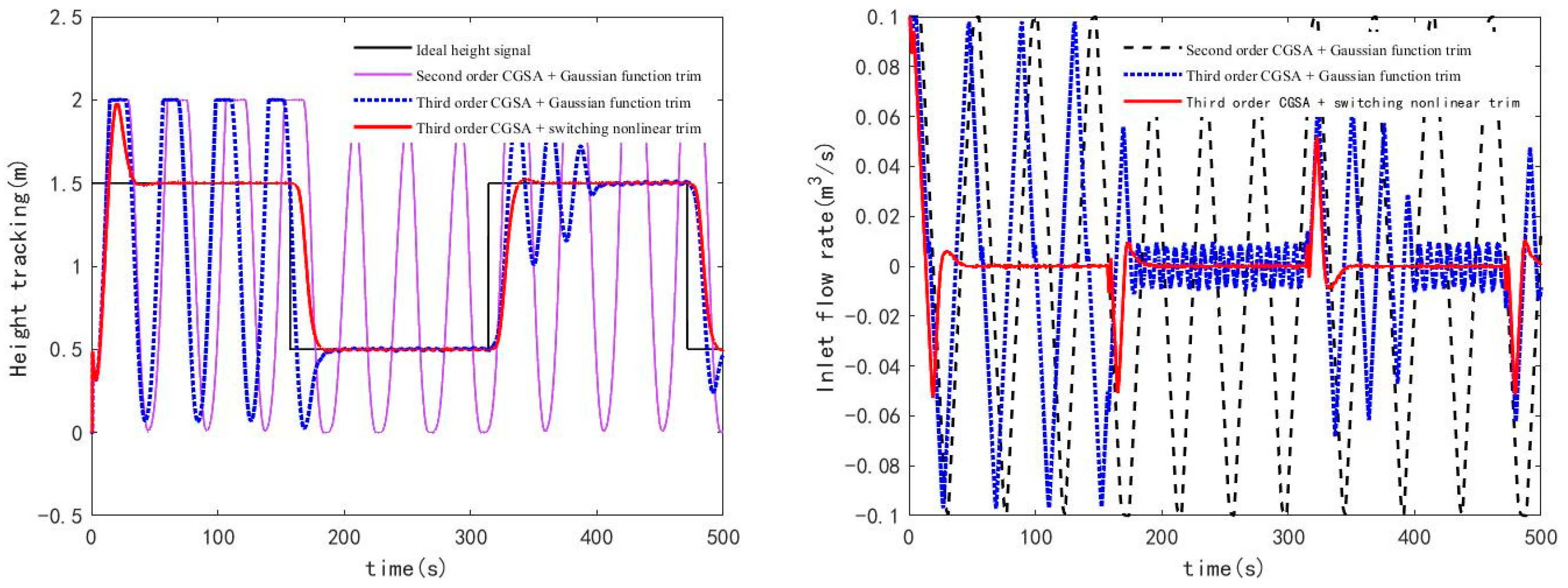
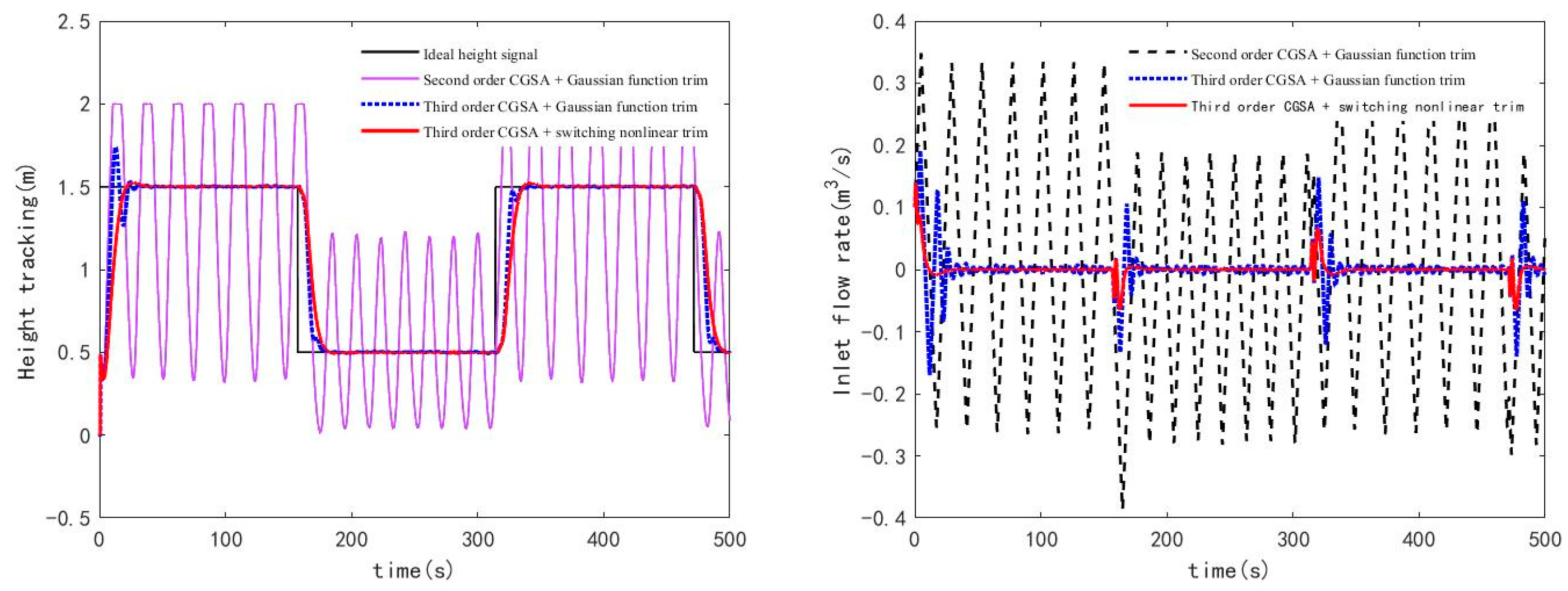
The set input signal for the level is a square wave that varies from 0.5 m to 1.5 m. We study the actual tank level control situation and find that there are limitations to both the tank inlet flow rate and the inlet acceleration. We introduce a servo system for the inlet water rate and acceleration to make the experiment fit the actual situation. We adopt the control variable method throughout the experiment. The conditions are as follows: (1) the objects are all hypothetical water tanks; (2) the simulation time is 500 s and the step size is set to 0.1 s; (3) the control parameter is ; (4) the non-linear switching modification parameters are , ; (5) the interference range simulated with white noise is ; (6) the maximum inlet flow rate is and the maximum inlet acceleration is . The control effects of small pump is shown in Figure 5.
From the above results(see Table 2), we can obtain that for the same non-linear modification function, the third-order CGSA has a reduction of more than 65% in each metric compared to the second-order CGSA. Therefore, the third-order CGSA has a more obvious advantage. Furthermore, the non-linear switch modification technique further reduces the three main indicators by 62%, 81%, and 67% compared to the Gaussian function. Then, to investigate the advantages of the improved model, we varied the maximum inlet flow rate and maximum inlet acceleration to simulate different types of pumps while maintaining the other experimental conditions. The maximum inlet flow rate is set to , and the maximum inlet acceleration is for next experiment. The control effects of large pump is shown in Figure 6.
From the above results(see Table 3), we can obtain that the MAE, MIA, and MTV of the third-order CGSA controller decreased by 84%, 91%, and 69%, compared to the controller with second-order CGSA in the case of the same non-linear modification function. In the case of the same order CGSA, the non-linear switching modification technique proposed in this paper results in a 70% and 74% decrease in the MIA and MTV, respectively, but a 20% increase in the MAE value compared to the Gaussian function. Notably, this is due to a decrease in response speed in comparison. However, the overshoot of the algorithm proposed in this paper decreases obviously, which is more significant for the actual control of the tank level. In summary, in the presence of time lag, a small amount of interference, pump speed limitations, etc., the third-order CGSA and non-linear switching modification techniques proposed in this paper have significant advantages in terms of control quality, energy savings, and algorithmic smoothness. The non-linear modified switching technique proposed in this paper performed well in both experiments. It shows that it works well for different types of water tanks. Therefore it has great application potential.
We listed two reasons for the energy-saving effect and smoothness of the controller proposed in this paper.
(1) The controller using second-order CGSA is equivalent to adding a first-order filtering component to PD control. The controller using third-order CGSA is equivalent to adding a second-order low-pass filter to the PD control. PD control will introduce high-frequency noise. High-frequency noise can be filtered by both first and second-order low-pass filters. However, the transition band of the second-order low-pass filter is narrower. Then unwanted interference signals will decay faster, and the noise is filtered out more cleanly. It can be verified by the better performance of the third-order CGSA controller for the same non-linear modifier function.
(2) Unlike non-linear modification techniques that sacrifice dynamic performance to reduce energy consumption, the non-linear switching modification technique proposed in this paper can selectively change the system gain. The dynamic performance of the system remains in the initial stage of the control process, and the control input decreases after reaching a steady state to reduce energy consumption.
6. Conclusions
This paper designs a concise and robust control scheme for water tank levels that can further improve the control quality. We first design a linear controller using a third-order closed-loop gain-shaping algorithm. The control law is then modified using a nonlinear switching modification technique based on an arcsine function. Additionally, the stability of the closed-loop system with time lag is demonstrated using the Nyquist stability criterion. We use a hypothetical tank model with a small disturbance, a pure lag of 0.8 s, and a pump servo system to verify the controller. Take one of the experiments as an example, compared to the second-order CGSA controller modified by the Gaussian function, the third-order CGSA controller modified by the nonlinear switch in this paper decreases by 81%, 97%, and 92% in MAE, MIA, and MIV. In the case of the same order CGSA, the MIA and MTV of the system with the non-linear switching modification technique reduce by 70% and 74%, respectively. Therefore, the controller reduces energy consumption and helps to extend the service life of the pump while maintaining a better control effect, which is of great significance to the actual large-size tank level control system. Finally, we give a theoretical analysis of the reasons for the excellent energy saving and smoothness of the controller in this paper. Compared with the second-order CGSA simple nonlinear technique, the control algorithm in this paper is more effective in filtering out high-frequency disturbances, which improves the energy-saving effect while further increasing the smoothness of the algorithm. In the future, we will automatically optimize the control parameters using energy saving and other indicators as constraints.
Author Contributions
Conceptualization, W.X. and H.W.; methodology, W.X.; software, W.X.; validation, X.Z. and W.X.; writing—original draft preparation, W.X.; writing—review and editing, W.X. and H.W.; supervision, X.Z. and W.X. All authors have read and agreed to the published version of the manuscript.
Funding
This research was funded by the National Science Foundation of China (Grant No. 51679024), Dalian Innovation Team Support Plan in the Key Research Field (Grant No. 2020RT08), and the Fundamental Research Funds for the Central University (Grant No. 3132021139).
Data Availability Statement
Not applicable.
Acknowledgments
Much appreciation to each reviewer for their valuable comments and suggestions to improve the quality of this note. The authors would like to thank anonymous reviewers for their valuable comments to improve the quality of this article.
Conflicts of Interest
The authors declare no conflict of interest.
References
- Li, L.; Li, J.; Gu, J.; Hua, L. Research on PID Control of Double Tank Based on QPSO Algorithm. Control. Eng. China 2021, 28, 1553–1558. [Google Scholar] [CrossRef]
- Zhang, X.; Jia, X. Robust PID Algorithm Based on Closed-Loop Gain Shaping and Its Application in Liquid level Control. Shipbuild. China 2000, 41, 37–41. [Google Scholar] [CrossRef]
- Zhao, K. Self-adaptive Fuzzy PID Control for Three-tank Water. In Proceedings of the 5th International Conference on Machine Vision (ICMV)-Algorithms, Pattern Recognition and Basic Technologies, Wuhan, China, 20–21 October 2012; p. 87841. [Google Scholar] [CrossRef]
- Cheng, Z.; Shi, Y.; Zhang, J.; Lv, C.; Qian, N.; Zhang, X.K. Research of liquid level control system based on fuzzy neural PID algorithm. Electron. Meas. Technol. 2019, 42, 29–34. [Google Scholar] [CrossRef]
- Olivas, E.L.; Castillo, O.; Soria, J.; Melin, P. A new methodology for membership function design using Ant Colony Optimization. In Proceedings of the IEEE Symposium on Swarm Intelligence (SIS), Singapore, 16–19 April 2013; pp. 40–47. [Google Scholar] [CrossRef]
- Young, K.D.; Utkin, V.I.; Ozguner, U. A control engineer’s guide to sliding mode control. IEEE Trans. Control. Syst. Technol. 1999, 7, 328–342. [Google Scholar] [CrossRef] [Green Version]
- Derdiyok, A.; Basci, A. The application of chattering-free sliding mode controller in coupled tank liquid-level control system. Korean J. Chem. Eng. 2013, 30, 540–545. [Google Scholar] [CrossRef]
- Mehri, E.; Tabatabaei, M. Control of quadruple tank process using an adaptive fractional-order sliding mode controller. J. Control. Autom. Electr. Syst. 2021, 32, 605–614. [Google Scholar] [CrossRef]
- Sekban, H.T.; Can, K.; Basci, A. Model-Based Dynamic Fractional-Order Sliding Mode Controller Design for Performance Analysis and Control of a Coupled Tank Liquid-Level System. Adv. Electr. Comput. Eng. 2020, 20, 93–100. [Google Scholar] [CrossRef]
- Moradi, H.; Saffar-Avval, M.; Bakhtiari-Nejad, F. Sliding mode control of drum water level in an industrial boiler unit with time varying parameters: A comparison with H-infinity-robust control approach. J. Process Control. 2012, 22, 1844–1855. [Google Scholar] [CrossRef]
- Zhang, Z.H.; Zhang, X.K. Controller Design for MIMO System with Time Delay Using Closed-loop Gain Shaping Algorithm. Int. J. Control. Autom. Syst. 2019, 17, 1454–1461. [Google Scholar] [CrossRef]
- Guan, W.; Zhang, X.K. Concise Robust Control for Ship Roll Motion Using Active Fins. Adv. Manuf. Syst. 2011, 201–203, 2366–2374. [Google Scholar] [CrossRef]
- Jiang, R.F.; Zhang, X.K. Application of Wireless Network Control to Course-Keeping for Ships. IEEE Access 2020, 8, 31674–31683. [Google Scholar] [CrossRef]
- Gao, S.H.; Zhang, X.K. Course keeping control strategy for large oil tankers based on nonlinear feedback of swish function. Ocean. Eng. 2022, 244, 110385. [Google Scholar] [CrossRef]
- Min, B.X.; Zhang, X.K.; Wang, Q. Energy Saving of Course Keeping for Ships Using CGSA and Nonlinear Decoration. IEEE Access 2020, 8, 141622–141631. [Google Scholar] [CrossRef]
- Zhang, Z.H.; Zhang, X.K.; Zhang, G.Q. ANFIS-based course-keeping control for ships using nonlinear feedback technique. J. Mar. Sci. Technol. 2019, 24, 1326–1333. [Google Scholar] [CrossRef]
- Zhang, X.K.; Yang, G.P.; Zhang, Q.; Zhang, G.Q.; Zhang, Y.Q. Improved Concise Backstepping Control of Course Keeping for Ships Using Nonlinear Feedback Technique. J. Navig. 2017, 70, 1401–1414. [Google Scholar] [CrossRef]
- Zhao, B.G.; Zhang, X.K.; Liang, C.L. A novel path-following control algorithm for surface vessels based on global course constraint and nonlinear feedback technology. Appl. Ocean. Res. 2021, 111, 102635. [Google Scholar] [CrossRef]
- Min, B.X.; Zhang, X.K. Concise robust fuzzy nonlinear feedback track keeping control for ships using multi-technique improved LOS guidance. Ocean. Eng. 2021, 224, 108734. [Google Scholar] [CrossRef]
- Su, Z.J.; Zhang, X.K. Nonlinear Feedback-Based Path Following Control for Underactuated Ships via an Improved Compound Line-of-Sight Guidance. IEEE Access 2021, 9, 81535–81545. [Google Scholar] [CrossRef]
- Cao, J.H.; Zhang, X.K.; Zou, X. Pressure Control of Insulation Space for Liquefied Natural Gas Carrier with Nonlinear Feedback Technique. J. Mar. Sci. Eng. 2018, 6, 133. [Google Scholar] [CrossRef] [Green Version]
- Song, C.Y.; Zhang, X.K.; Zhang, G.Q. Nonlinear innovation identification of ship response model via the hyperbolic tangent function. Proc. Inst. Mech. Eng. Part I J. Syst. Control. Eng. 2021, 235, 977–983. [Google Scholar] [CrossRef]
- Zhao, J.; Zhang, X.K. Inverse Tangent Functional Nonlinear Feedback Control and Its Application to Water Tank Level Control. Processes 2020, 8, 347. [Google Scholar] [CrossRef] [Green Version]
- Zhao, J.; Zhang, X.K.; Chen, Y.L.; Wang, P.R. Using Sine Function-Based Nonlinear Feedback to Control Water Tank Level. Energies 2021, 14, 7602. [Google Scholar] [CrossRef]
- Zhang, X.K.; Song, C.Y. Robust Controller Decorated by Nonlinear S Function and Its Application to Water Tank. Appl. Syst. Innov. 2021, 4, 64. [Google Scholar] [CrossRef]
- Zhao, Z.J.; Zhang, X.K.; Li, Z. Tank-Level Control of Liquefied Natural Gas Carrier Based on Gaussian Function Nonlinear Decoration. J. Mar. Sci. Eng. 2020, 8, 695. [Google Scholar] [CrossRef]
- Zhang, X.K.; Zhang, G.Q. Nonlinear Feedback Theory and Its Application to Ship Motion Control; Dalian Maritime University Press: Dalian, China, 2000; pp. 135–136. [Google Scholar]
Figure 1.
Configuration diagram of level keeping control based on nonlinear switch decoration.

Figure 2.
Typical S&T singular value curve.

Figure 3.
Amplitude phase characteristic curve of controller.

Figure 4.
Amplitude phase characteristic curve of system.

Figure 5.
The control effects of small pump.

Figure 6.
The control effects of large pump.


Table 1.
Notations and descriptions.
| Notations | Descriptions |
|---|---|
| Steady-state value of input water flow | |
| Increment of input water flow | |
| Steady-state value of output water flow | |
| Increment of output water flow | |
| Liquid level height | |
| Steady-state value of the liquid level | |
| Increment of liquid level | |
| Regulating the opening of valves | |
| Cross-sectional area of the water tank | |
| Resistance of load valves at the outflow end | |
| Change in opening of control valve |
Table 2.
Controller performance of small map.
| Control Method | MAE | MIA | MTV |
|---|---|---|---|
| Second order CGSA + Gaussian function trim | 0.7347 | 0.0566 | 0.0009 |
| Third order CGSA + Gaussian function trim | 0.3107 | 0.0260 | 0.0009 |
| Third order CGSA + Switching nonlinear trim | 0.1167 | 0.0049 | 0.0003 |
Table 3.
Controller performance of large pump.
| Control Method | MAE | MIA | MTV |
|---|---|---|---|
| Second order CGSA + Gaussian function trim | 0.5121 | 0.1452 | 0.0049 |
| Third order CGSA + Gaussian function trim | 0.0795 | 0.0129 | 0.0015 |
| Third order CGSA + Switching nonlinear trim | 0.0956 | 0.0039 | 0.0004 |
Disclaimer/Publisher’s Note: The statements, opinions and data contained in all publications are solely those of the individual author(s) and contributor(s) and not of MDPI and/or the editor(s). MDPI and/or the editor(s) disclaim responsibility for any injury to people or property resulting from any ideas, methods, instructions or products referred to in the content. |
© 2023 by the authors. Licensee MDPI, Basel, Switzerland. This article is an open access article distributed under the terms and conditions of the Creative Commons Attribution (CC BY) license (https://creativecommons.org/licenses/by/4.0/).
Share and Cite
MDPI and ACS Style
Xu, W.; Zhang, X.; Wang, H. A Water Tank Level Control System with Time Lag Using CGSA and Nonlinear Switch Decoration. Appl. Syst. Innov. 2023, 6, 12. https://doi.org/10.3390/asi6010012
AMA Style
Xu W, Zhang X, Wang H. A Water Tank Level Control System with Time Lag Using CGSA and Nonlinear Switch Decoration. Applied System Innovation. 2023; 6(1):12. https://doi.org/10.3390/asi6010012
Chicago/Turabian StyleXu, Weifeng, Xianku Zhang, and Haoze Wang. 2023. "A Water Tank Level Control System with Time Lag Using CGSA and Nonlinear Switch Decoration" Applied System Innovation 6, no. 1: 12. https://doi.org/10.3390/asi6010012