Tree-Structured Model with Unbiased Variable Selection and Interaction Detection for Ranking Data

Abstract

In this article, we propose a tree-structured method for either complete or partial rank data that incorporates covariate information into the analysis. We use conditional independence tests based on hierarchical log-linear models for three-way contingency tables to select split variables and cut points, and apply a simple Bonferroni rule to declare whether a node worths splitting or not. Through simulations, we also demonstrate that the proposed method is unbiased and effective in selecting informative split variables. Our proposed method can be applied across various fields to provide a flexible and robust framework for analyzing rank data and understanding how various factors affect individual judgments on ranking. This can help improve the quality of products or services and assist with informed decision making.

1. Introduction

Tree-structured methods, such as classification and regression trees, are important techniques in machine learning and data mining [1,2,3]. They are widely used in various applications, including image and speech recognition, natural language processing, and medical diagnosis. One of the main reasons for their popularity is their ability to handle complex data and extract meaningful insights from it. Classification trees are used to predict the class of a new observation based on its features or attributes. They work by recursively partitioning the data into smaller and more homogeneous groups based on the values of the features. The resulting tree can be interpreted to understand which features are most important in determining the class of the observation. This is useful in many applications, such as credit risk assessment, where the goal is to predict whether a borrower will default on a loan. Regression trees, on the other hand, are used to predict a continuous variable, such as the price of a house or the stock price of a company, based on a set of predictor variables. They work by recursively partitioning the data into smaller groups based on the values of the predictors. The resulting tree can be interpreted to understand how the predictor variables affect the outcome variable. This is useful in many applications, such as financial forecasting, where the goal is to predict future prices based on historical data. Tree-based methods are also important because they are non-parametric, meaning they do not make assumptions about the underlying distribution of the data. This makes them robust to outliers and noise in the data. Additionally, they can handle both categorical and continuous variables, as well as missing values.

Rank data are frequently collected in various fields, such as education [4], psychology [5], health care [6], quality of life [7], sociology [8], and marketing [9], with the main motivation being to understand how people perceive and evaluate a set of items or alternatives. This information can be used to make informed decisions and improve the quality of products or services. However, in some cases, the complete rank of the items may not be available, and only the top-k ranking outcomes are observed. This poses a challenge for data analysis, as traditional statistical methods are not suitable for dealing with rank data. In addition, some related covariates are also collected to understand how these variables affect the judgment of each individual on ranking [10,11]. The goal of the research presented in the article is to develop statistical methods for analyzing top-k rank data and related covariates. The focus is on understanding how various factors affect the judgment of each individual on ranking. For instance, in marketing, understanding how demographic variables such as age, gender, and income affect consumer preferences can help companies tailor their products to specific target markets, while in healthcare, understanding how patient characteristics such as age, gender, and health status affect their perception of the quality of care can help improve healthcare services. The research also aims to address some of the challenges associated with analyzing rank data, such as how to handle ties and missing data, and how to incorporate covariate information into the analysis. The ultimate goal is to provide a flexible and robust framework for analyzing rank data that can be applied across various fields.

Lee and Yu [12], Yu et al. [13], and Plaia [14] proposed decision tree models for rank data. In their tree models, the exhaustive search principle of CART [1] based on either some distance-based models [12] or impurity measures [15] is applied to select splits. The pruning method is later applied to select the right-sized tree. Only the method based on impurity measures can handle either complete or partial rank data ([12]). Cheng et al. [16] also proposed a tree induction method using the same exhaustive search principle for either type of rank data, but only numerical covariates are allowed. A direct stopping rule is then applied to select the final tree. Kung et al. [17] show that the distance-based tree models tend to select variables with more split points. They propose a relatively unbiased selection method which utilizes the conditional independence tests based on log-linear models for contingency tables. However, complete ranks are required in their paper.

In this paper, we propose a tree-structured method for either complete or partial rank data. The method relies on the observation that if the response variable is not related to its covariates, then the item numbers become independent of the covariates given the corresponding ranks. We leverage this fact by using conditional independence tests based on hierarchical log-linear models for three-way contingency tables [18] to choose the split variables and cut points. We use Pearson’s chi-squared tests of independence to guide split variables and points selection. A Bonferroni type stopping rule is applied to declare a node terminal. Through simulation, our method is shown to be relatively unbiased and more effective in selecting the informative split variables.

2. Materials and Methods

2.1. Dataset

The European Values Study (EVS) is a large-scale survey conducted every nine years to examine the attitudes, beliefs, and values of people in various countries across Europe. The time span for each survey may vary, and the collected data may cover different themes and questions. The countries included in the EVS survey also vary depending on the edition of the study, but generally, they cover a wide range of European countries. We would apply our tree method to analyzing a sample of the 1999 EVS data containing an assessment of materialism/postmaterialism in 3584 respondents from 32 countries. We follow the suggestion from Vermunt [19] and divide the countries into four groups for the 1999 EVS data. The main reason for dividing the countries into four regions is to account for potential cultural and contextual differences between them. By controlling for the potential impact of regional differences, survey data can be analyzed more accurately. The respondents were asked to pick the most important and the second most important goals for their Government from the following four alternatives: (A) Maintain order in nation; (B) Give people more say in government decisions; (C) Fight rising prices; and (D) Protect freedom of speech. Eight covariates are associated with each response and they are country group (CG), gender (G), year of birth (Y), age of education completion (ED), marital status (M), employment status (EM), occupation (O), and household income (I). Individuals can be classified into three groups based on their choices. Regardless of the ordering, individuals who prefer (A) and (C) are classified as “materialist”, whereas those who prefer (B) and (D) are classified as “postmaterialist”. The rest of the individuals are classified as those holding “mixed” value orientations [19]. The dataset is obtained from R package psychotree [20]. There are missing values in the data. After removing missing values, there are a total of 1911 respondents from 26 countries with complete data information, and the country group is given in

Table 1. The country groups in the EVS data without missing values. The value in parentheses is the number of respondents.

Group	Country
1	Italy (113), the Netherlands (48), Denmark (95)
2	France (106), Spain (35), Belgium (115), Croatia (24), Greece (53)
3	West Germany (52), East Germany (48), Iceland (62), Czechia (144),
	Romania (60), Bulgaria (64), Malta (29), Luxembourg (32), Slovenia (49)
4	Estonia (70), Latvia (66), Lithuania (50), Poland (109), Slovakia (103),
	Hungary (77), Russia (170), Ukraine (66), Belarus (71)

.

2.2. Variable Selection

We first introduce the Gini impurity measure, which is used in Yu et al. [13] to select split variables and points. The Gini impurity measure is a way of quantifying the impurity of a set of examples, which is used to determine the best way to split the data at each level of the decision tree. The goal is to minimize the Gini impurity at each split, resulting in more homogeneous subsets of data that are easier to classify. We often refer to methods using such techniques as exhaustive searches. Exhaustive search of choices refers to the process of considering all possible ways of splitting the data at each level of the tree in order to identify the best split that minimizes the Gini impurity.

The Gini impurity measure for rank data is defined as follows. Given m items, let $C^{m,d}$, $d\le m$ be the set of ranking with members from all possible d-permutations of m elements in $\{1,2,\dots ,m\}$. Suppose only top $-k$ rank outcomes, $k\le m$, are observed. For node t, let $p(y_1,\dots ,y_k|t)$ be the proportion of cases where item $y_1$ ranks first, item $y_2$ ranks second, and so on. The top-k Gini index is defined as:

$$i^{\left(k\right)}\left(t\right)=1-\sum _{\pi \in C^{m,k}}p{\left(\pi \right|t)}^2.$$

when $k=m$, it becomes the usual Gini index [1], where each of the $m!$ rank outcomes is treated as a class.

For each covariate X, a split of the form $X<c$, if X is an ordered variable; or $X\in S$, if X is a categorical variable, is considered. Such split creates subnode $t_l$ and $t_r$. All possible constants c or subsets S are considered and the split which minimizes the following:

$$i_X^{\left(k\right)}\left(t\right)=N_{t_l}{i}^{\left(k\right)}\left(t_l\right)+N_{t_r}{i}^{\left(k\right)}\left(t_r\right)$$

which is chosen to be the best split associated with X, where $N_j$ is the sample size at node j, $j=t_l$ or $t_r$. The variable associated with the minimal value of $i_X^{\left(k\right)}\left(t\right)$ is the split variable at node t. We denote this method as the Gini method.

However, it is well known that the exhaustive search principle used in split variable selection has some disadvantages. Loh [3] provided some evidence for this in the context of classification and regression trees. Namely, the method has selection bias toward variables with more split points and it is costly to build such trees. Moreover, in their simulation study, Lee and Yu [12] and Kung et al. [17] found the evidence of such selection bias for trees used to model complete rank data.

To eliminate possible selection bias, a useful strategy is to separate variable selection from point selection. Loh and Shih [21] and Loh [22] have shown its effectiveness in classification and regression trees. A similar approach is taken by Kung et al. [17] for complete rank data. We follow the same principle and propose the following method to select split variables. For top-k ranking outcomes, we know there are at most $\kappa =m\times (m-1)\dots \times (m-k+1)$ different rank outcomes. We treat each of them as a class and use Pearson’s chi-squared independence test to guide the variable selection process. If a covariate is associated with the rank response, the test itself should reveal the degree of association. We denote our method as the ST (Statistical Test) method. The algorithms, called Algorithms 1 and 2, are given in what follows. Denote $p_s$ and $p_s^{\ast }$ as two probability values.

Algorithm 1 Main effect detection.

For each ordered covariate, divide the data into four levels at the sample quartiles; construct a two-way $4\times \kappa$ contingency table with the levels as rows, the different ranking responses as columns; omit entries with zero column totals and count the number in each cell. Compute the Pearson chi-squared statistic of testing independence between the row and the column variable and obtain its corresponding p-value, denoted by $p_s$. Do the same for each categorical covariate, using the categories of the covariate to form the rows of the contingency table and omitting entries with zero row or column totals. The covariate which has the corresponding smallest $p_s$ value is chosen to be the split variable.

Algorithm 1 is designed to capture a single covariate effect, but it may lose its power when an interaction effect between two covariates appears [17]. To detect such interaction effects, we provide the following Algorithm 2.

Algorithm 2 Interaction effect detection.

Repeat Algorithm 1 and obtain the corresponding $p_s$ value. For a pair of ordered covariates $(X_i,X_j)$, divide the $(X_i,X_j)$-space into four quadrants by split the range of each variable into two halves at the sample median; construct a two-way $4\times \kappa$ contingency table with the quadrants as rows, and the different ranking responses as columns; omit entries with zero column totals and count the number in each cell. Do the same for each pair of categorical covariates, using their categorical pairs to form the rows of the contingency table and omit entries with zero row or column totals. For each pair of covariates $(X_i,X_j)$ where $X_i$ is ordered and $X_j$ is categorical, divide the $X_i$-space into two categories at the sample median; use their categorical pairs to form the rows of the contingency table and omit entries with zero row or column totals. Obtain its corresponding p-value. For each pair of covariates, denote the smallest p-value be $p_s^{\ast }$. If $p_s^{\ast }<p_s$, the (interaction) covariate with the smaller $p_s$ value is chosen to be the split variable. Otherwise, the covariate which has the corresponding smallest $p_s$ value is chosen.

2.3. Point Selection and Stopping Rule

After the split variable is selected, the split point is determined by applying Algorithm 1 as follows. For each possible split point, samples are divided into two subnodes. By treating two subnodes as two rows in the contingency table analysis used in Algorithm 1, we obtain a p-value for each point. The point associated with the smallest p-value is then selected as the split point.

We employ a simple Bonferroni rule to determine whether a node worths splitting or not. A node stops splitting if its p-value associated with the split point is not less than $\alpha /N_c$, where $\alpha$ is a pre-specified probability value and $N_c$ is the number of available cut point at the node. We set $\alpha =0.01$ in our data analysis. Besides, a node with the sample size of its child node smaller than a fixed number is not split. This fixed value is set to be 20 in our data analysis.

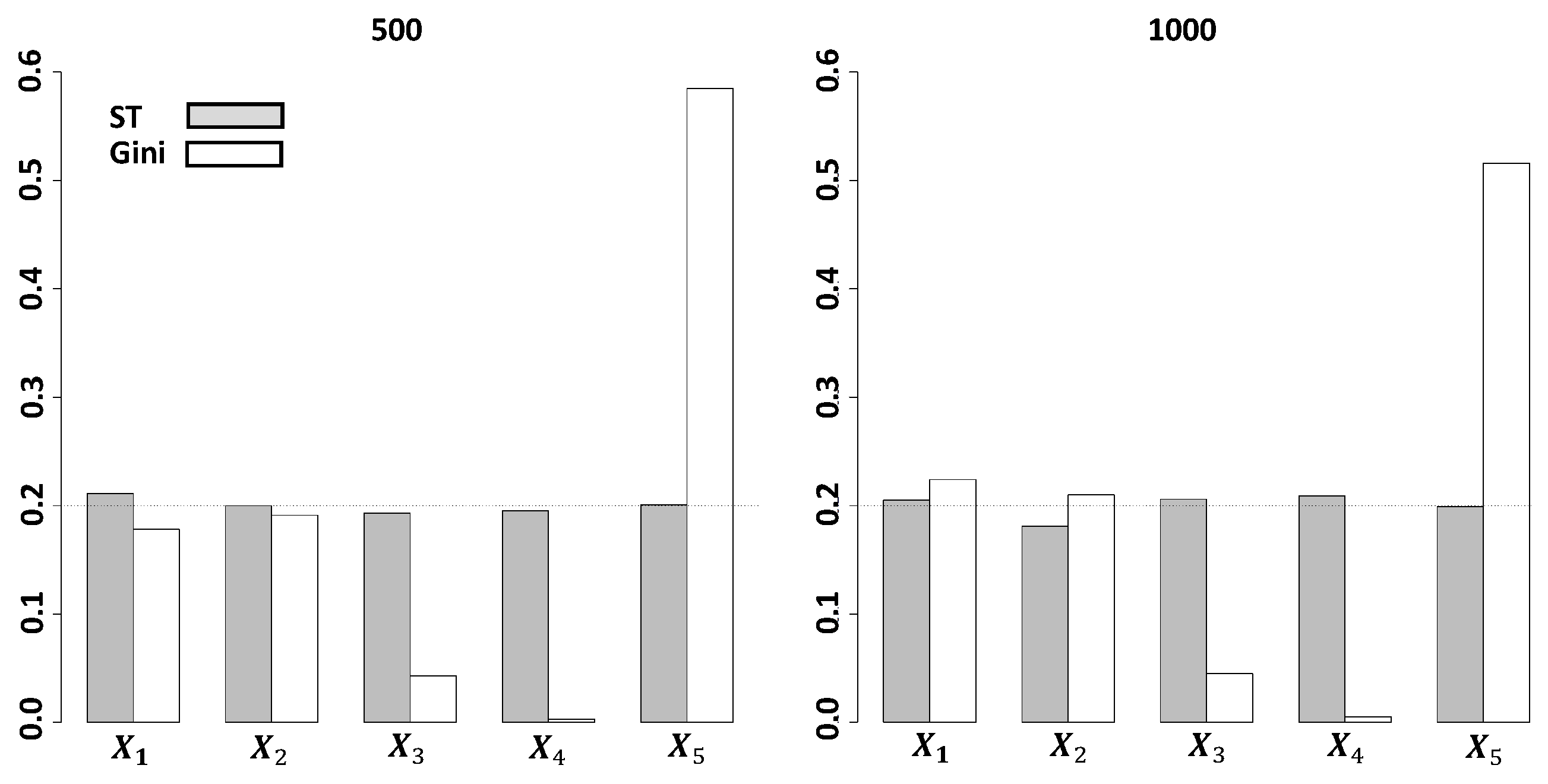
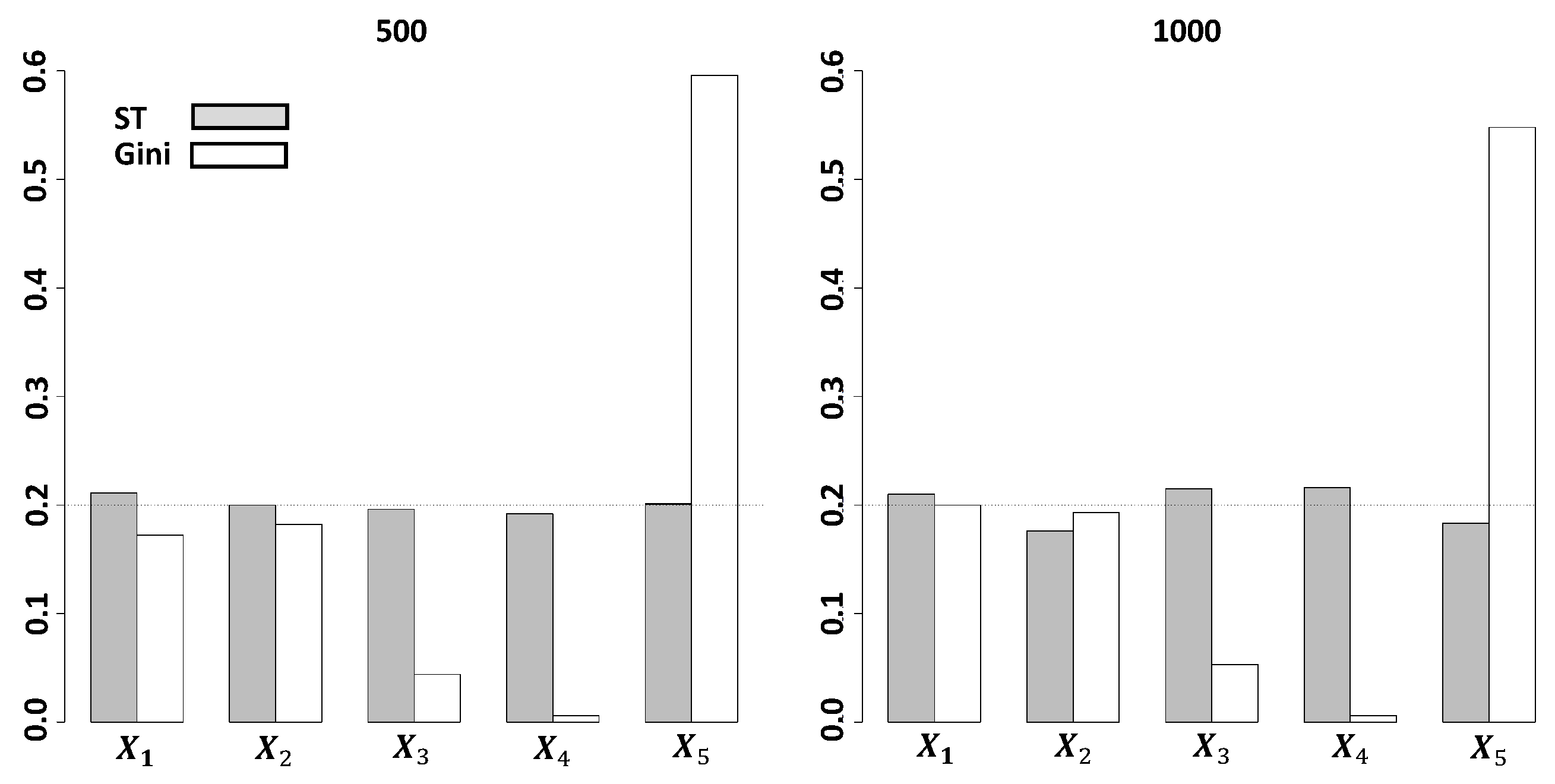
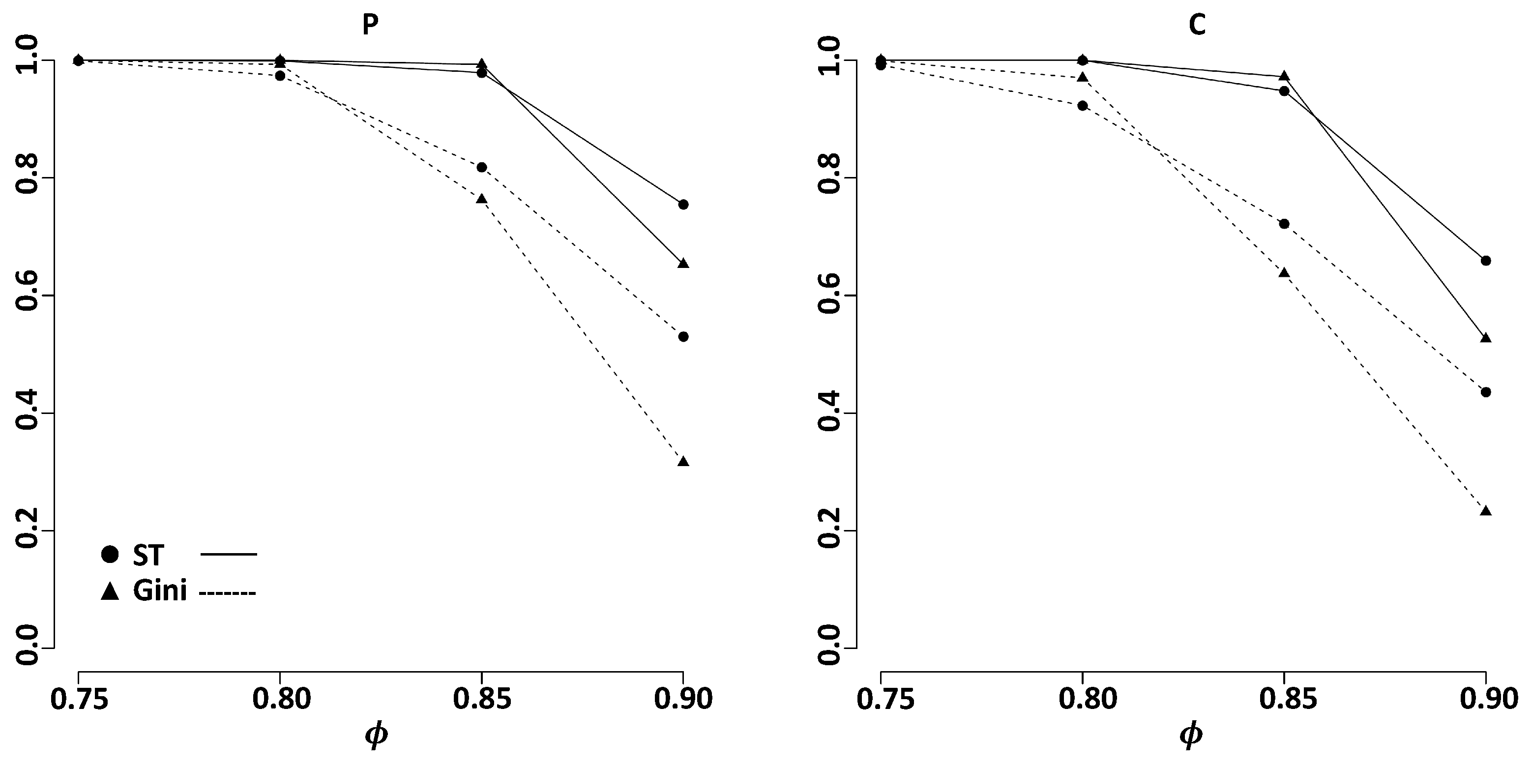
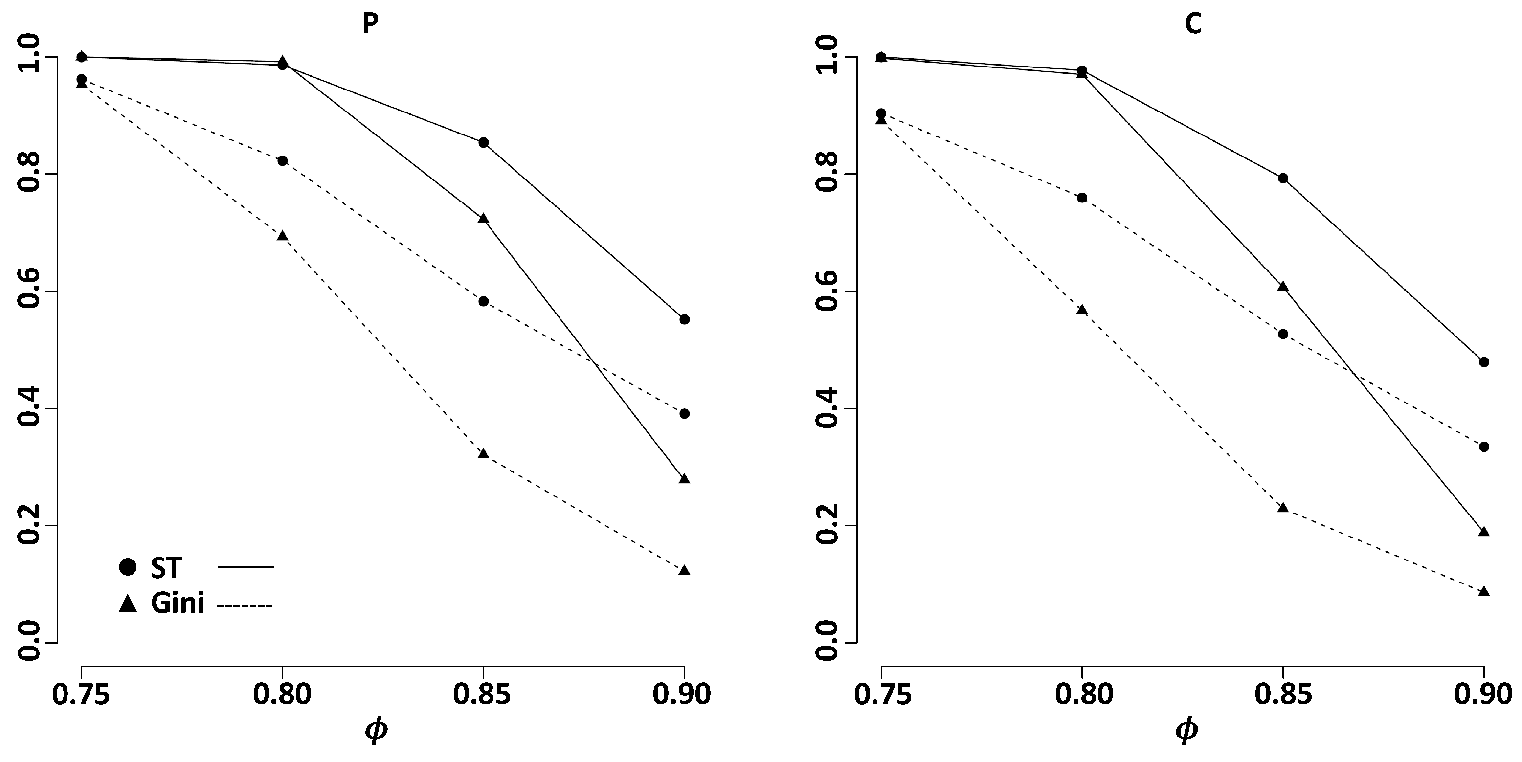
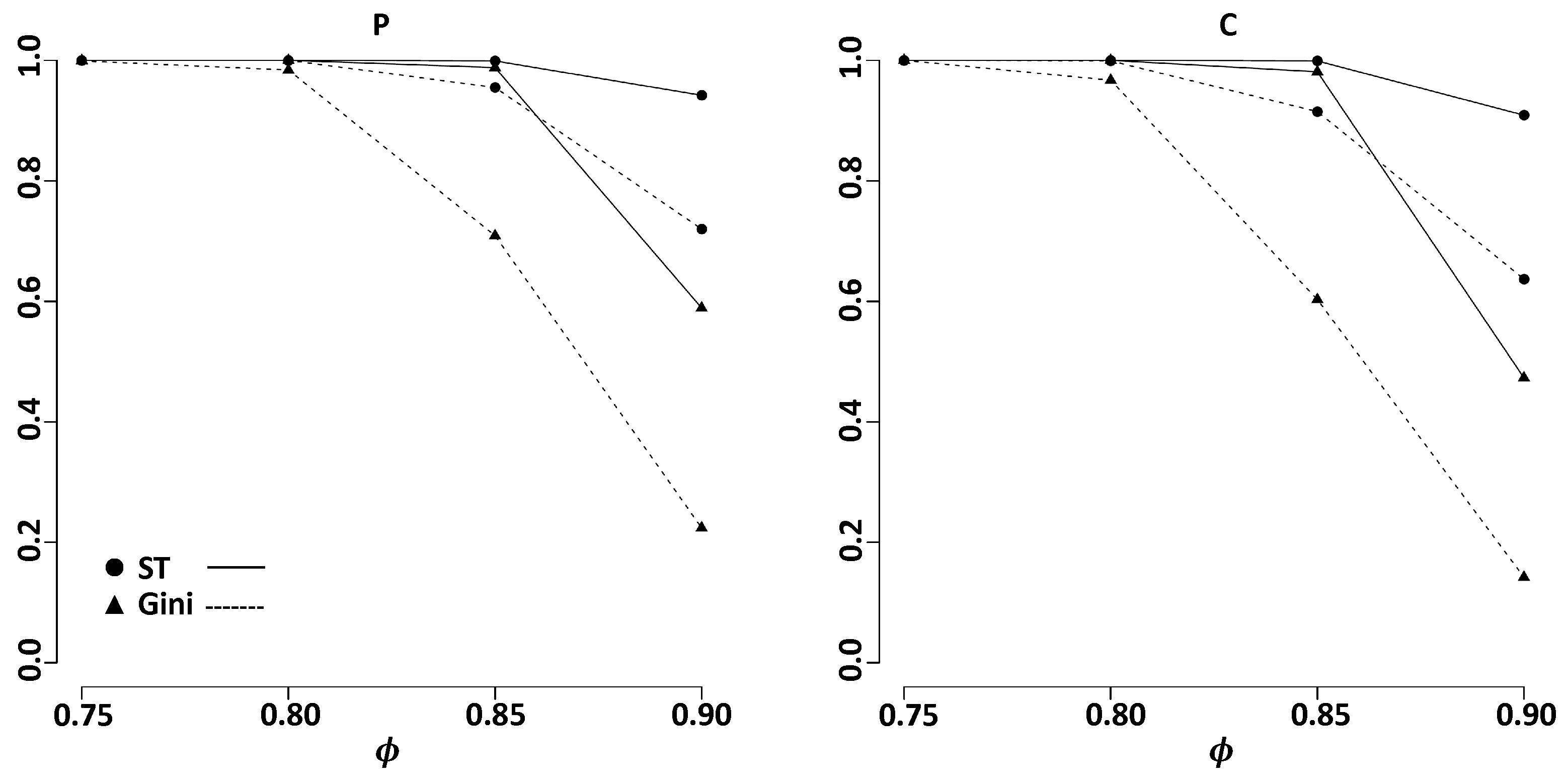
3. Simulation Studies on Variable Selection

We compare the Gini and the ST methods on variable selection in this section. Rank samples are generated by using the following Kendall’s tau distance-based model. For k items with label $1,\dots ,k$, let $\pi$ be a rank function from $\{1,\dots ,k\}$ onto $\{1,\dots ,k\}$, where $\pi \left(i\right)$ is the rank of item i. The class of distance-based models(DBM) for rank data proposed by Diaconis [23] is as follows:

$$\mathrm{Pr}\left(\pi \right|\lambda ,{\pi }_0)=e^{-\lambda d(\pi ,{\pi }_0)}\times C{\left(\lambda \right)}^{-1}$$

(1)

where $\lambda \ge 0$ is the dispersion parameter, $d(\pi ,{\pi }_0)$ is a distance function between ranking function $\pi$ and ${\pi }_0$, and $C\left(\lambda \right)$ is a proportionality constant. Let $\varphi =e^{-\lambda }$. The closer to the modal ranking ${\pi }_0$ is, the higher probability of occurrence ranking has. The distribution of ranking will be more concentrated around ${\pi }_0$ for smaller $\lambda$ (larger $\varphi$). Kendall’s tau distance is considered and it is defined as:

$$d({\pi }_1,{\pi }_2)=\sum _{i<j}I\{[{\pi }_1\left(i\right)-{\pi }_1\left(j\right)][{\pi }_2\left(i\right)-{\pi }_2\left(j\right)]<0\},$$

where $I(·)$ is an indicator function and ${\pi }_1$ and ${\pi }_2$ are rank functions for $i,j\in \{1,\dots ,k\}$.

Suppose $\mathbf{Y}$ is the response variable with ranking outcome 1, 2, 3, or 4. Two types of the response samples are considered. One is complete rank and the other is partial rank. For the partial rank responses, the last two rank values are deleted after the associated complete rank responses are simulated. Five independent covariates are also used and their distributions are given in

Table 2. Distributions of X variables used in the simulation studies. Z, E, $U_{10}$, $C_2$, and $C_{10}$ are mutually independent; Z is a standard normal variable; E is an exponential variable with mean one; $U_{10}$ is a uniformly distributed variable on the set $\{1,2,\dots ,10\}$; $C_m$ denotes an m-category variable taking values $\{1,2,\dots ,m\}$ with equal probabilities.

$X_1\sim Z$

$X_2\sim E$

$X_3\sim U_{10}$

$X_4\sim C_2$

$X_5\sim C_{10}$

. Among them, the first three are ordered and the others are categorical covariates. For each study, 500 or 1000 random samples of $\mathbf{Y}$ and its related covariates are generated, respectively. The number of times of each covariate selected by the Gini and ST methods are recorded in 1000 repetitions.

3.1. Independent Case

In this study, the response variable is designed to be independent of the five covariates. The response is generated by Kendall’s tau distance-based model with $\varphi =0.8$. The estimated probability for each covariate being selected is given in Figure 1 and Figure 2 for partial (top-2) rank and complete rank responses, respectively.

From both figures, we find that the Gini method select $X_1$ or $X_2$ more frequently than $X_3$ for ordered covariates. For categorical covariates, it selects $X_5$ more often than $X_4$. For either sample sizes (500 or 1000), it is designed that $X_1$ or $X_2$ has more split points than $X_3$, as does $X_4$ compared with $X_5$. Hence, we find that the Gini method tends to select variables with more split points. However, in this study, the response variable is assumed to be independent of the five covariates. The probability of each variable being selected must be approximately 1/5. Therefore, we believe that the Gine method has obvious variable selection bias. Conversely, the ST method selects each covariate all within three standard errors of 1/5 for each design setting. We conclude that our method is relatively unbiased.

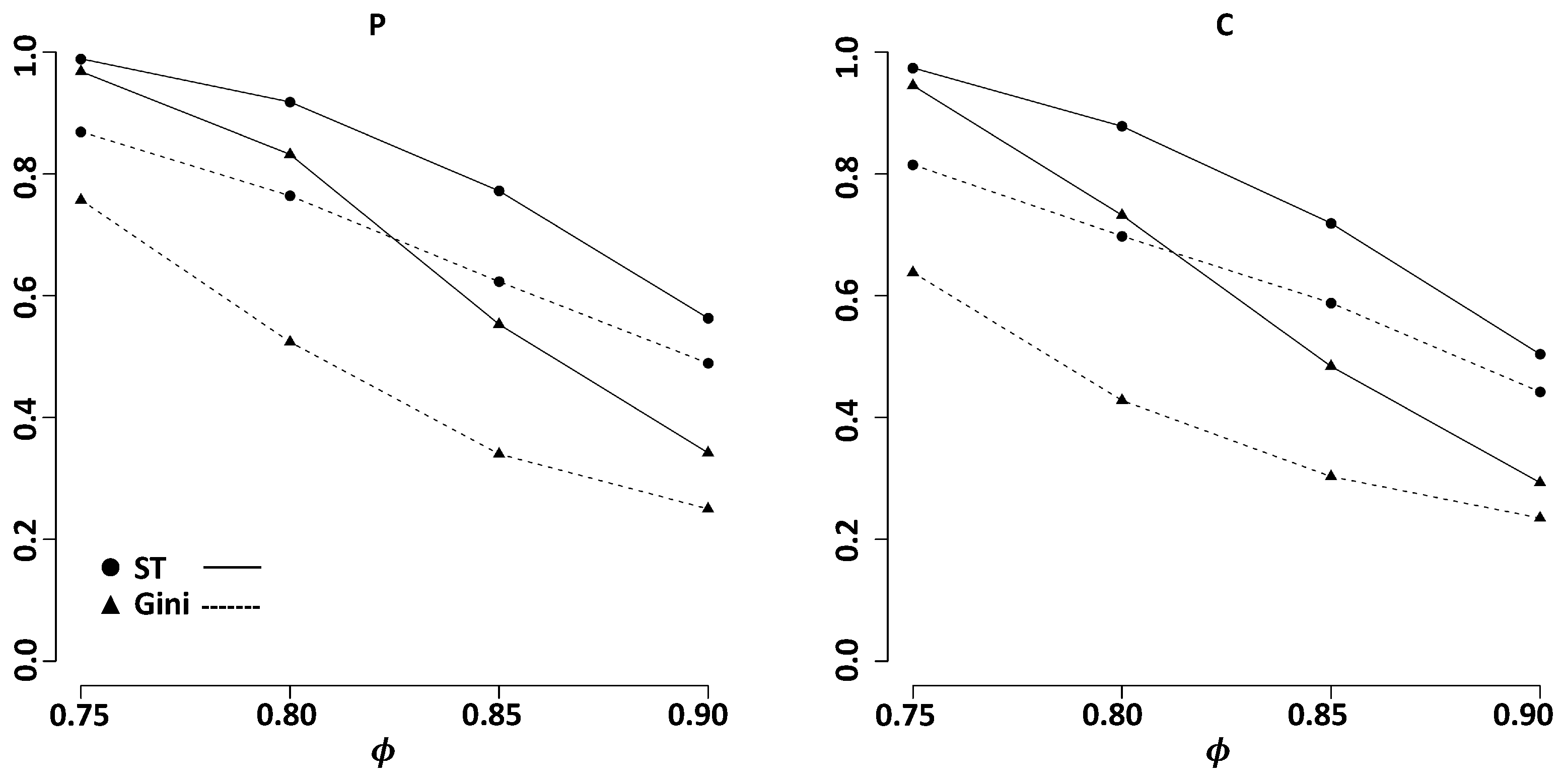
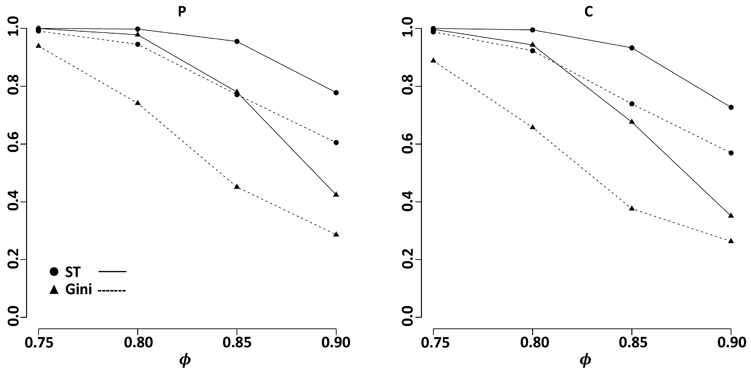
3.2. Dependent Models

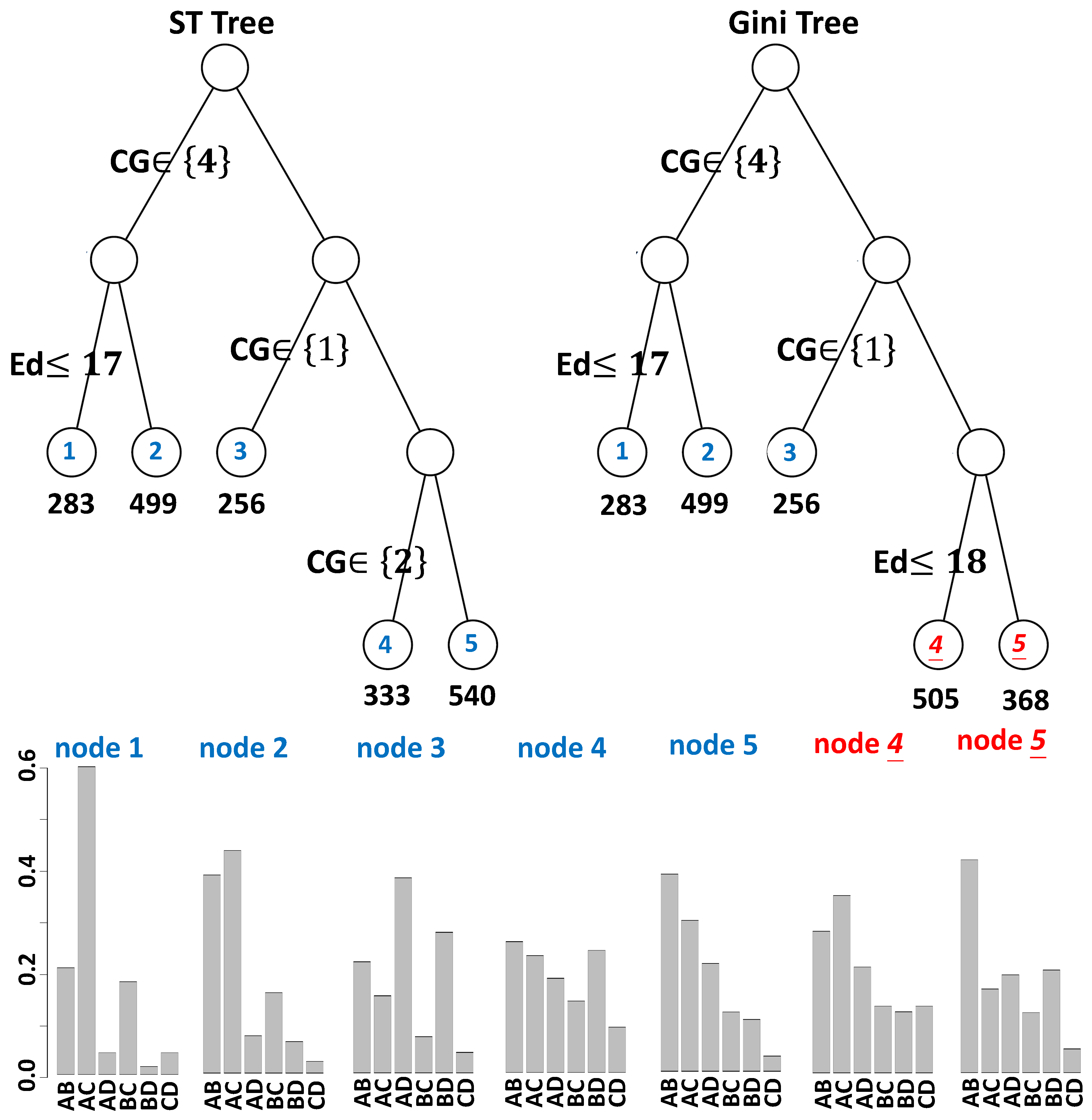
We study the selection power of the two methods in this section. The response variables, which depend on some covariates, are generated. Five dependent models are considered and they are given in

Table 3. Models for power studies of the variable selection methods. The response variable is generated by fitting Kendall’s tau distance-based model with ${\pi }_0=(1,2,3,4)$ when the condition is satisfied; otherwise, ${\pi }_0=(4,3,2,1)$. The distributions of X values are given in Table 2, $S=\left\{(X_2,X_4)\right|X_2\le 1\mathrm{or}{X}_4\in \left\{1\right\}\}$, and $T=\left\{(X_2,X_4)\right|X_2\le 1\mathrm{and}{X}_4\in \left\{1\right\}\}$.

Model	Condition
I	$X_3\le 5$
II	$|X_3-5|\le 2$
II	$X_4\in \left\{1\right\}$
IV	$(X_2,X_4)\in S$
V	$(X_2,X_4)\in T$

. For example, in Model I, when $X_3\le 5$, rank outcomes are generated by fitting Kendall’s tau distance model with ${\pi }_0=(1,2,3,4)$. Otherwise, they are generated with ${\pi }_0=(4,3,2,1)$. Each of the first four models only contains a main effect, while the last model involves a pure interaction effect. The estimated probability for informative covariate(s) being selected is recorded and the results are given in Figure 3, Figure 4, Figure 5, Figure 6 and Figure 7, respectively.

For Model I, a mean shift in $X_3$ changes the response. Therefore, $X_3$ is an important factor in Model I and should be defined as a selection variable. From Figure 3, we observe that the Gini method performs slightly better than the ST method for $\varphi \le 0.8$. This trend continues for $\varphi =0.85$ when the sample size is 1000. However, for $\varphi =0.85$ and the sample size is 500 or $\varphi =0.9$, the ST method is better.

For Model II, a range change in $X_3$ affects the response. To ensure the accuracy, it is crucial to choose $X_3$ as a selection variable. Figure 4 indicates that the Gini method is compatible with the ST method when $\varphi =0.75$. Otherwise, the ST method performs better than the Gini method. Moreover, for some values of $\varphi$, the selection probabilities of the Gini method are smaller than 1/5, which is undesirable. The selection bias of the Gini method contributes to this.

The response depends on $X_4$ under Model III. Therefore, $X_4$ holds great significance in Model III and we should define $X_4$ as a selection variable. From Figure 5, we find that the Gini method is competitive with the ST method when $\varphi =0.75$. For larger $\pi$ values, the selection probability of the Gini method drops rather fast and its performance is inferior to the ST method.

Under Model IV, either $X_2$ or $X_4$ is informative. Using $X_2$ or $X_4$ as a selection variable is imperative for the model to produce reliable outcomes. Figure 6 shows that the ST method is always better than the Gini method in selecting the informative variables for the settings with either partial or complete rank outcomes.

For Model V, it involves an interaction effect between $X_2$ and $X_4$. According to the literature proposed by Kung et al., when there is an interaction effect between variables, utilizing a strategy of interaction detection such as Algorithm 2 will result in more powerful outcomes. Therefore, we test Algorithm 2 against the Gini method in this study. To keep the effectiveness of Model V, either $X_2$ or $X_4$ should be assigned as a selection variable. Figure 7 shows that the ST method using Algorithm 2 is able to select the correct variables more effectively than the Gini method.

Through these studies, we conclude that the ST method is more reliable in selecting the informative variables than the Gini method, except perhaps some cases in Model I.

4. Data Analysis

We apply our method to the EVS data and its resulting tree is shown in Figure 8. The bar plots of each terminal shows the proportions of combined partial rank responses in each terminal node. For the convenience of representation, we regard A&B and B&A as the same category. In other words, the label assigns a rank to outcomes regardless of their order, for instance, AB indicates that the ranking is either A&B or B&A. We find that country group and age of education completion are two decisive predictors, which agrees with the finding of Lee and Yu (2010). However, the selection of split variables differs between the fourth and fifth nodes. In the ST method, there is only one cut point selection for the CG variable, whereas in the Gini method, there are more cut point selections for the Ed variable (in fact, 32 cut points). This confirms the discussion of the dependent models in Section 3.2, which shows that the Gini method favors the split variable with more cut points. Therefore, in our analysis of the EVS data, we have more confidence in the ST tree method. Group 4 countries are in node 1 and 2, which are divided by education level. Node 3, 4, and 5 consist of Group 1, 2, and 3 countries, respectively. From the bar plots, we further notice that, regardless of the ordering, the majority of individuals in Group 4 prefer (A) and (C), and individuals with higher education level (Ed > 17) valued (A) and (B) almost as important as (A) and (C). For Group 1 countries, people prefer (A) and (D), while people in Group 3 give priority to (A) and (B). For Group 2 countries, although people prefer (A) and (B), almost equal preference is given to (B) and (D) or (A) and (C).

5. Conclusions

Decision trees are excellent data exploratory tools. In this article, we propose a framework of constructing decision trees for rank data which may contain missing ranks. It uses Pearson’s chi-squared tests of independence to select the split variable as well as its split point at each node. It retains its nature of easy interpretation without worrying about the split selection bias. Through simulation experiments, we find that, compared with the Gini criterion method of Yu et al. [13], our selection method is relatively unbiased. Furthermore, it is more effective in selecting the informative covariates when these covariates are related to the ranking response. A Bonferroni type stopping rule is applied to declare a node terminal. In the end, our tree method is used to analyze an EVS dataset and some distinct ranking patterns are found.

Two issues are not treated in this paper. One is the assignment rule of terminal nodes. It surely depends on the criterion, which can be (1) mean rank, (2) top-choice frequency, (3) the most frequently observed rank, or (4) the paired comparison probabilities [13]. The other issue is the assessment of tree performance, which may rely on (a) deviance [12], (b) AUC [13], or (c) Kendall’s tau statistics [16]. This will be the subject of our future research.

References

1. Breiman, L.; Friedman, J.H.; Olshen, R.A.; Stone, C.J. Classification and Regression Trees, 1st ed.; Chapman & Hall: New York, NY, USA, 1984. [Google Scholar]
2. Buri, M.; Tanadini, L.G.; Hothorn, T.; Curt, A. Unbiased Recursive Partitioning Enables Robust and Reliable Outcome Prediction in Acute Spinal Cord Injury. J. Neurotrauma 2022, 39, 266–276. [Google Scholar] [CrossRef] [PubMed]
3. Loh, W.Y. Classification and regression trees. Wiley Interdiscip. Rev. Data Min. Knowl. Discov. 2011, 1, 14–23. [Google Scholar] [CrossRef]
4. Acuña-Soto, C.; Liern, V.; Pérez-Gladish, B. Normalization in TOPSIS-based approaches with data of different nature: Application to the ranking of mathematical videos. Ann. Oper. Res. 2021, 296, 541–569. [Google Scholar] [CrossRef]
5. Handayani, D.O.D.; Lubis, M.; Lubis, A.R. Prediction analysis of the happiness ranking of countries based on macro level factors. Int. J. Artif. Intell. 2022, 11, 666–678. [Google Scholar] [CrossRef]
6. Hackert, M.Q.N.; Brouwer, W.B.F.; Hoefman, R.J.; van Exel, J. Views of older people in the Netherlands on wellbeing: A Q-methodology study. Soc. Sci. Med. 2019, 240, 1–9. [Google Scholar] [CrossRef] [PubMed]
7. Patil, G.R.; Sharma, G. Urban Quality of Life: An assessment and ranking for Indian cities. Transp. Policy 2022, 124, 183–191. [Google Scholar] [CrossRef]
8. Harakawa, R. Ranking of importance measures of tweet communities: Application to keyword extraction from COVID-19 tweets in Japan. IEEE Trans. Comput. Soc. Syst. 2021, 8, 1029–1040. [Google Scholar] [CrossRef] [PubMed]
9. Adlakha, K.; Sharma, S. Brand positioning using Multidimensional Scaling technique: An application to herbal healthcare brands in Indian market. J. Bus. Perspect. 2020, 24, 345–355. [Google Scholar] [CrossRef]
10. Finch, H. An introduction to the analysis of ranked response data. Pract. Assess. Res. Eval. 2022, 27, 7. [Google Scholar]
11. Marden, J.I. Analyzing and Modeling Rank Data, 1st ed.; Chapman & Hall: New York, NY, USA, 1996. [Google Scholar]
12. Lee, P.H.; Philip, L.H. Distance-based tree models for ranking data. Comput. Stat. Data Anal. 2010, 54, 1672–1682. [Google Scholar] [CrossRef]
13. Yu, P.L.H.; Gu, J.; Xu, H. Analysis of ranking data. Wiley Interdiscip. Rev. Comput. Stat. 2019, 11, e1483. [Google Scholar] [CrossRef]
14. Plaia, A.; Sciandra, M. Weighted distance-based trees for ranking data. Adv. Data Anal. Classif. 2019, 13, 427–444. [Google Scholar] [CrossRef]
15. Yu, P.L.H.; Wan, W.M.; Lee, P.H. Decision Tree Modeling for Ranking Data; Fürnkranz, J., Hüllermeier, E., Eds.; Preference Learning; Springer: Berlin/Heidelberg, Germany, 2010; pp. 83–106. [Google Scholar]
16. Cheng, W.; Hühn, J.; Hüllermeier, E. Decision tree and instance-based learning for label ranking. In Proceedings of the 26th Annual International Conference on Machine Learning, Montreal, QC, Canada, 14–18 June 2009; pp. 161–168. [Google Scholar]
17. Kung, Y.H.; Lin, C.T.; Shih, Y.S. Split variable selection for tree modeling on rank data. Comput. Stat. Data Anal. 2012, 56, 2830–2836. [Google Scholar] [CrossRef]
18. Simonoff, J.S. Analyzing Categorical Data; Springer: New York, NY, USA, 2003. [Google Scholar]
19. Vermunt, J. Multilevel latent class models. Sociol. Methodol. 2003, 33, 213–239. [Google Scholar] [CrossRef]
20. Strobl, C.; Wickelmaier, F.; Zeileis, A. Accounting for individual differences in Bradley-Terry models by means of recursive partitioning. J. Educ. Behav. Stat. 2011, 36, 135–153. [Google Scholar] [CrossRef]
21. Loh, W.Y.; Shih, Y.S. Split selection methods for classification trees. Stat. Sin. 1997, 7, 815–840. [Google Scholar]
22. Loh, W.Y. Regression trees with unbiased variable selection and interaction detection. Stat. Sin. 2002, 12, 361–386. [Google Scholar]
23. Diaconis, P. Group Representations in Probability and Statistics. Lect. Notes-Monogr. Ser. 1988, 11, i-192. [Google Scholar]
Figure 1. Estimated probabilities of variable selection for the ST and the Gini method where Y is independent of the X values. The sample size is 500 and 1000, respectively. The distribution of Y follows the DBM model with Kendall’s tau distance function, where ϕ = 0.8 and π 0 = ( 1 , 2 , 3 , 4 ) . The top-2 rank data are used in this setting. The distributions of X values are given in Table 2. The simulation standard errors are about 0.018.
Make 05 00027 g001
Figure 2. Estimated probabilities of variable selection for the ST and the Gini method, where Y is independent of the X values. The sample size is 500 and 1000, respectively. The distribution of Y follows the DBM model with Kendall’s tau distance function, where ϕ = 0.8 and π 0 = ( 1 , 2 , 3 , 4 ) . The complete rank data are used in this setting. The distributions of X values are given in Table 2. The simulation standard errors are about 0.018.
Make 05 00027 g002
Figure 3. Estimated probability of X 3 is selected for the ST and the Gini method under Model I. Data are observed for partial rank (P, top-2) or complete rank (C) and the sample size is 500 or 1000.
Make 05 00027 g003
Figure 4. Estimated probability of X 3 is selected for the ST and the Gini method under Model II. Data are observed for partial rank (P, top-2) or complete rank (C) and the sample size is 500 or 1000.
Make 05 00027 g004
Figure 5. Estimated probability of X 4 is selected for the ST and the Gini method under Model III. Data are observed for partial rank (P, top-2) or complete rank (C) and the sample size is 500 or 1000.
Make 05 00027 g005
Figure 6. Estimated probability of X 2 or X 4 is selected for the ST and the Gini method under Model IV. Data are observed for partial rank (P, top-2) or complete rank (C) and the sample size is 500 or 1000.
Make 05 00027 g006
Figure 7. Estimated probability of X 2 or X 4 is selected for the ST and the Gini method under Model V. Data are observed for partial rank (P, top-2) or complete rank (C) and the sample size is 500 or 1000.
Make 05 00027 g007
Figure 8. ST tree and Gini tree for EVS data. At each intermediate node, an observation goes to the left child node if and only if the stated condition is satisfied. The number beneath each terminal node gives the node sample size.
Make 05 00027 g008