Article

A Reinforcement Learning Approach for Scheduling Problems with Improved Generalization through Order Swapping

1
ScaliRo GmbH, Eduard-Rüber-Straße 7, 83022 Rosenheim, Germany
2
Faculty of Management and Engineering, Rosenheim Technical University of Applied Sciences, Hochschulstraße 1, 83024 Rosenheim, Germany
*
Author to whom correspondence should be addressed.
Mach. Learn. Knowl. Extr. 2023, 5(2), 418-430; https://doi.org/10.3390/make5020025
Submission received: 3 April 2023 / Revised: 25 April 2023 / Accepted: 27 April 2023 / Published: 29 April 2023

Abstract

:
The scheduling of production resources (such as associating jobs to machines) plays a vital role for the manufacturing industry not only for saving energy, but also for increasing the overall efficiency. Among the different job scheduling problems, the Job Shop Scheduling Problem (JSSP) is addressed in this work. JSSP falls into the category of NP-hard Combinatorial Optimization Problem (COP), in which solving the problem through exhaustive search becomes unfeasible. Simple heuristics such as First-In, First-Out, Largest Processing Time First and metaheuristics such as taboo search are often adopted to solve the problem by truncating the search space. The viability of the methods becomes inefficient for large problem sizes as it is either far from the optimum or time consuming. In recent years, the research towards using Deep Reinforcement Learning (DRL) to solve COPs has gained interest and has shown promising results in terms of solution quality and computational efficiency. In this work, we provide an novel approach to solve the JSSP examining the objectives generalization and solution effectiveness using DRL. In particular, we employ the Proximal Policy Optimization (PPO) algorithm that adopts the policy-gradient paradigm that is found to perform well in the constrained dispatching of jobs. We incorporated a new method called Order Swapping Mechanism (OSM) in the environment to achieve better generalized learning of the problem. The performance of the presented approach is analyzed in depth by using a set of available benchmark instances and comparing our results with the work of other groups.

1. Introduction

Scheduling problems in the field of manufacturing are usually distinguished in one of the three categories: (1) JSSP, (2) flow shop, and (3) open shop. This work addresses JSSPs, which are highly challenging, of significant industrial relevance, and often used as a benchmark for testing/comparing new methodologies. In JSSPs, every job has a fixed machine sequence that has to be followed during the production of the particular product [1]. Moreover, the job shop has n jobs  J 0 , J 1 , J 2 , , J n  that must be processed on m machines with every job-machine pair having a specific processing time that is given by the problem formulation. As the number of jobs and machines increases, combinatorial possibilities quickly explode and computation time of exhaustive searches become unfeasible even for medium-sized problems. It is worth noting that many COPs are considered to fall into the class of NP-hard problems, although this is not true for all instances. Moreover, conventional COPs and JSSPs exhibit distinct characteristics in terms of their problem formulation, solution space and constraints. This creates challenges when it comes to desgining effective representations that can capture these differences efficiently [2].
DRL is a subfield of machine learning where an agent is trained based on experience that is gathered from the interaction with an uncertain environment. The agent improves its performance by maximizing a reward signal that characterizes the overall goal such as reaching the shortest makespan in a production [3]. Lately, some remarkable milestones in the field of AI have been reached by employing DRL, such as outperforming the human in popular challenges such as the board game Go (AlphaGO [4]) or StarCraft II (AlphaStar [5]). The implementation of DRL in the field of Operational Research has become quite significant. Several studies incorporating DRL to solve COP have shown promising results [6,7,8,9]. Moreover, DRL provides a significantly faster approximation for COPs compared to exhaustive search, metaheuristics, or other conventional heuristics. In this paper, we propose a DRL based approach to efficiently solve the JSSP. We developed an efficient, problem-generic environment for arbitrary JSSP problems in OpenAI’s Gym framework. Along with the optimal reward modelling and compact state representation of the JSSP environment, the policy parameters of the policy network were trained to approach a deterministic policy. Based on the proposed approach, the PPO algorithm was tested by solving classical benchmark problems such as Taillard [10], and Demirkol et al. [11]. The performance of our trained network is compared with state-of-the-art algorithms regarding their achieved makespan (time to complete all operations).

2. Background

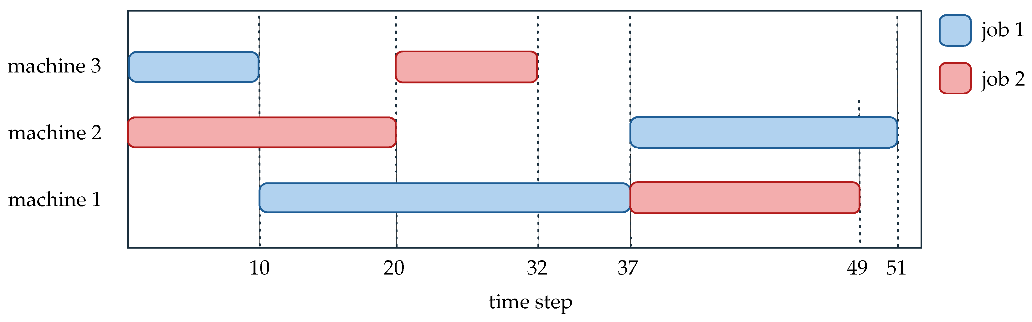
2.1. Job Shop Constraints

JSSPs consist of n jobs that need be processed on m machines. Each job has a particular processing scheme specifying the particular machining steps in a strict order. Moreover, every job-to-machine combination has a particular processing time on each machine. The total number of operations equals  O n × m . Each operation is indicated by  O i j  and their respective processing time is  d i j  where  i ( 1 , m )  and  j ( 1 , n ) . Conventionally, each job has a predetermined processing order that has to be followed to complete all operations. The order of a particular job can be represented as:
J j = { O j 1 d j 1 , O j 2 d j 2 , , O j m d j m } , for j ( 1 , n ) , m ( 1 , m ) .
based on the problem definition, the machining sequence is developed and the quality of the solution is evaluated by the makespan value. The machine up-time can be calculated using
T i = j = 1 n d i j .
The free time—or idling time—f for a machine correlates with the makespan as follows:
C max = max i ( j = 1 n ( d i j ) + f i ) .
The difficulty in finding the global optimum solution (lower bound) increases exponentially with the problem size  n × m .

2.2. Proximal Policy Optimization (PPO)

PPO is a policy gradient method that uses sampled data obtained from environment interaction in order to optimize the surrogate objective function using stochastic gradient ascent [12]. In comparison to Q-learning or Trust Region Policy Optimization, PPO is more data efficient, robust and less complex to implement. The surrogate objective function  L CLIP  of PPO is given by
L CLIP ( θ ) = E ^ t min ( r t ( θ ) A ^ t , clip ( r t ( θ ) , 1 ϵ , 1 + ϵ ) A ^ t ) .
The PPO objective is a clipped surrogate function that balances the tradeoff between policy improvement and stability. Note that the term clipping denotes that large gradients—and thus updates—are cut off to prevent catastrophic forgetting during the training process, and hence effectively limits the stability and convergence of the training process. The objective function is an expectation implying that we consider batches of trajectories to assess the agent’s performance. The term  r t ( θ ) A ^ t  is the unclipped update (the default term that is used in policy gradient methods) that steers the actions towards high advantages over the baseline. The second term term  clip ( r t ( θ ) , 1 ϵ , 1 + ϵ ) A ^ t  is a clipped version of the normal policy gradient objective and is employed to control the magnitude of policy updates by constraining the new policy to be close to the old policy.  ϵ  is a hyperparameter that controls the range of the update and is usually in the magnitude order of  0.2 . The minimum of both terms is used to prevent that updates based on the improvement of the objective function become too large. Finally, the objective function is optimized using ordinary gradient-based optimization methods such as stochastic gradient descent.

3. Related Works

Although research adressing JSSPs is rather sparse, several different algorithms have been employed to attain their specific optimization goals. Algorithms such as taboo search [13], simulated annealing [14], genetic algorithms and particle swarm optimization [15] have been frequently used by other groups to solve JSSPs. However, these methodologies usually have a great tradeoff between computation time and problem size and moreover, usually feature low generalization capabilities. Advancements in DRL approaches in recent years have enabled considerable progress for the domain of COP applications [16,17]. Some of the major COPs have been successfully solved using DRL such as the Travelling Salesman Problem [18,19,20], the Knapsack Problem [7,16] and the Steiner Tree Problem [6]. Zhang and Dietterich [21] were able to show the potential of Reinforcement Learning for JSSPs as far back as 1995, by improving the results of the scheduling algorithm by Deale et al. [22] which used a temporal difference algorithm in combination with simulated annealing. Manerba et al. [8] give a comprehensive overview of traditional reinforcement learning algorithms for scheduling problems. Further, the study from Gabel and Riedmiller [23] on using a gradient descent policy search method for scheduling problems demonstrated the feasibility of DRL in JSSPs. Despite the reduced computation time, the solution found was not better than that of traditional solvers. This limitation was partially overcome by Liu et al. [24], who designed an environment based on a Multi-Agent Markov Decision Process and used a Deep Deterministic Policy Gradient for their approach. The agent performed well on the smaller instances, producing a good scheduling score of around 90% but eventually, the performance declined with the increase in size of the instances. To deal with the increased complexity of the problem, an Adaptive Job Shop Scheduling based on a Dueling Double Deep Q-Network with a prioritized reply was proposed by Han and Yang [25]. The authors used a disjunctive graph-based model to design the environment and transform it into a sequential decision-making problem. The algorithm was tested for generalization ability by training the network with random events in the existing environment to quickly adapt to new problems. However, the agent was not tested with a completely new dataset, an issue which was overcome by Zhang et al. [2]. The authors developed a graph neural network which enabled them to solve size-agnostic problems. Similar to the previous approach the authors used a disjunctive  g r a p h = ( , C , D )  with being the chosen operation of the JSSP  = { O i j | i , j } { S , T } , C the set of directed arcs and D the set of undirected arcs, to represent the state space of the JSSP. The performance of the agent was promising, although the generalized results were far off from the optimum. To handle this, Tassel et al. [26] proposed a new DRL algorithm to solve the JSSPs with compact state space representation and a simple dense reward function. The action space was designed for n jobs along with an additional job called No-Op (No Operation). The agent was tested with different benchmark instances where the agent performed around 18% better than Zhang et al. [2] and 10% better than Han and Yang [25]. Even though they provide a near-optimum solution, the approach falls short of the generalization objective. The motive of our approach is to develop an efficient environment that can perform better in both the objectives i.e., generalization and near-optimum solutions.

4. Methodologies

The job shop environment is built with OpenAI Gym which provides modules to develop a reinforcement learning environment. An agent learns to solve the environment and optimize the parameters of the policy by interacting with it through actions.

4.1. Environment Outline

Along with the mathematical constraints explained before, the environment is designed with further constraints [1,27]:
  • No pre-emption is allowed i.e., operations cannot be interrupted
  • Each machine can handle only one job at a time
  • No precedence constraints among operations of different jobs
  • Fixed machine sequences of each job
For example, when considering a JSSP with three machines and two jobs with a job order  J 1 = { 3 , 1 , 2 } , J 2 = { 2 , 3 , 1 }  the environment treats each operation as an atomic operation (cannot be interrupted). So once the job  J 0  is assigned on machine  M 3  at time step 0 it cannot be interrupted till time step 10, as shown in Figure 1.
Based on the described problem definition, we consider the JSSP as a single agent problem. Additionally, it has been shown by Tassel et al. [26] that the performance of the single agent DRL outperforms existing state-of-the-art DRL methods. Unlike Tassel et al.’s approach, our implementation of the environment has a different environmental design with no additional action (No-Op) and no non-final prioritization technique.

4.2. Time Step Transition

For the efficient learning of the agent, the time step and machines to be assigned are chosen based on the eligibility of operation. This enables the environment to provide the agent with only the potential requests at which machines can be assigned. At each chosen time step, the environment fetches all eligible operations O based on the provided job order of the problem. The definition of an eligible operation relies on the job order and the current state of the jobs and machines. For example, consider the previously discussed job shop problem with three machines and two jobs, with total operations  m × n = 6 . The set of operations can be expressed as
O = { O 11 J 1 M 3 , O 12 J 1 M 1 , O 13 J 1 M 2 , O 21 J 2 M 2 , O 22 J 2 M 3 , O 23 J 2 M 1 }
along with the set of processing times
d = { d 11 10 , d 12 27 , d 13 14 , d 21 20 , d 22 12 , d 23 12 } .
Based on the predetermined job order, the eligible operations are  O 11  and  O 21  at time step 0 and similarly, at time step 10, the eligible operation is limited to  O 12 . Likewise, the time step where the agent will be queried next in the environment is chosen based on the minimum length of the operation which is currently active. This enables the program to skip unnecessary checks for run time length in order to determine the next operation. At time step 0, the active operations are  O 11 O 21  with corresponding times  d 11 d 21  of length 10 and 20. The environment then directly jumps to time step 10 which is minimum operation length of the currently running operations  O 11 O 21 . The transition is further regulated by the availability of the machines and jobs at the future time step. For instance, at time step 20, operations  O 12 O 22  are active until time step 32 and 37. Even though the operation  O 22  has the minimum processing time, jumping to time step 32 will not be useful, since the next operation  O 23  which involves processing job  J 2  on machine  M 1  is not eligible at time step 32 as the machine  M 1  is processing job  J 1  till 37. So the environment directly jumps to the time step 37. With this mode of time step transition and querying mechanism, the agent was able to solve the JSSP environment by taking steps approximately equal to the total number of operations. To put this into perspective, the jobs of the Taillard [10] ta01 instance with 15 machines and 15 jobs was completed with 225 requests that is equivalent to the total number of operations. Exploiting this mechanism, a significant improvement can be reached. During the initial phase of training, the agent’s numerous action requests to solve the problem are often ineffective, resulting in increased training time. To mitigate this issue, a roll-out buffer is implemented, which incorporates episodic termination after a certain number of time steps. The roll-out buffer is a manually chosen hyperparameter and correlates with the complexity of the problem.

4.3. Action Space

The environment is controlled by a single discrete action space. With this action space, the agent determines the suitable job to process for a particular machine at each step. The agent is constrained to the set of jobs available
A t = { J 1 , J 2 , J 3 , , J n } .

4.4. States

At each time step, the state space is updated with the current status information of all jobs and machines. We developed a dictionary state space which incorporates the following information: (1) status of the machines—a boolean vector of size m indicating which machines are busy and idling, (2) operation progression—a vector of size m holding information on whether or not an operation is still running, (3) current remaining jobs—a vector of size n that shows the remaining operations per job, (4) overall operation overview—a two dimensional boolean array of size  n × m  that provides the status of the operations, (5) availability of jobs—a vector of size n that indicates the next eligible operation, (6) current machine processing information—a vector of size m that holds information regarding the currently processed jobs on the machine.

4.5. Reward

The reward function must closely correspond to the scheduling goal, e.g., guiding the suitable assignment of jobs to the appropriate machines and reducing the makespan of the schedule. It has been clearly shown in several studies that the performance of an agent with dense rewards is better than the performance of an agent with sparse rewards [28]. In this work, we have designed a simple dense reward function R to provide a feedback regarding the operation assignment and a final reward  R f  to express the viability of the achieved goal. Therefore the cumulative reward equals
R cumulative = a R + R f
R ( a t , s t ) = 1 , if O is a valid assignments 0 , else
The final reward  R f  is only given when the agent is successful in assigning all operations before the roll-out buffer is full. We employed the following equation:
R f = ( roll - out   buffer + α C m a x * ) · C 0 .
The equation can be easily interpreted by considering that the hyperparameter  α  is zero and  C 0  is unity; in this case, the equation simply states that the final reward starts at zero when the makespan is exactly the roll-out buffer. However, this is not a good scenario as the agent is not rewarded for solving the problem when the roll-out buffer and the makespan are in the same order of magnitude. We hence decided to introduce  α  that increases the final reward by a base value that is always given when the agent achieves to complete all jobs before the upper limit (given by the roll-out buffer) is reached. Hence,  α  can be seen as constant reward for completing the environment. Beyond this base reward, the agent gets higher rewards a lower the achieved makespan gets. Moreover,  C 0  serves as a factor to scale the final reward to increase/decrease it’s importance in comparison to the cumulative dense reward.

4.6. Markov Decision Process Formulation
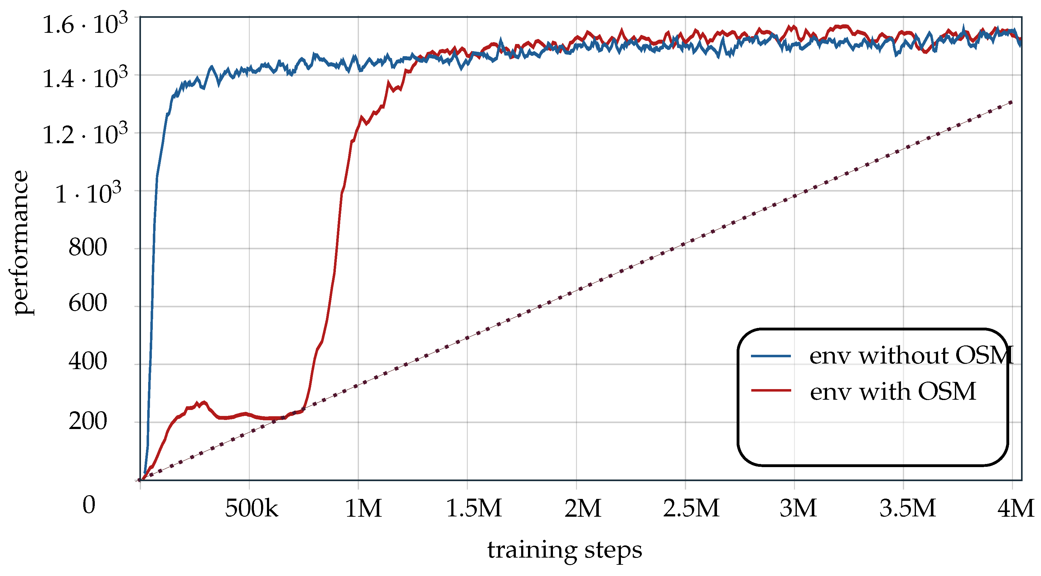
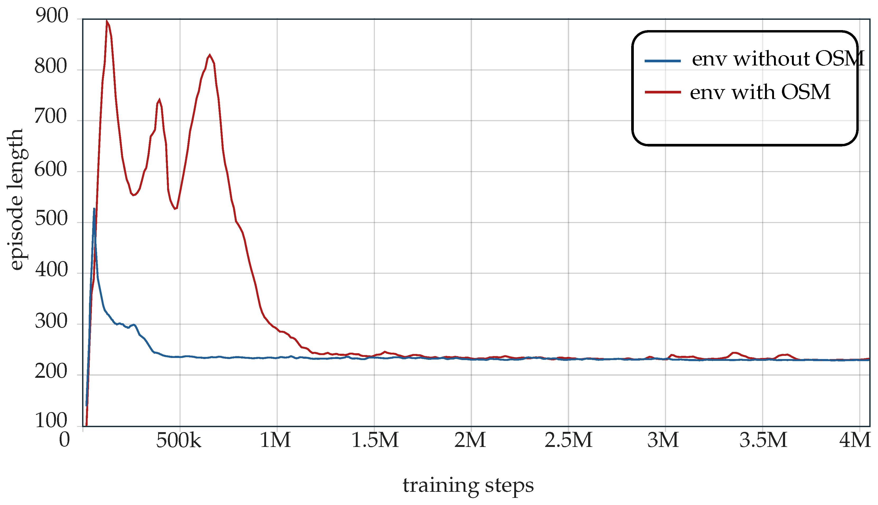
The JSSP can be modelled as a Markov Decision Process (MDP) since the assignment of the job sequentially changes the environment in terms of states and rewards, therefore the Markov property is fulfilled. JSSPs have been formulated as MDPs in several previous studies [2,25,26,29,30] with different approaches based on the type of algorithm used to solve the problem. The agent assigns a job through an action  a t  at time step t and retrieves the next state  s t + 1 . Unlike single assignment at a time step t, there can also be multiple assignments based on the number of eligible operations k at time step t. The actions at time step t are given by  a t 0 , a t 1 , , a t k  extending the state space at t by  s t 0 , s t 1 , , s t k . The probability of the next state is modified based on the sub actions taken at the time step. This can be expressed by
p ( s , r | s , a ) = P r { S t = s , R t = r | S t 1 = s , A t 1 = a } .

4.7. Generalization

In order to increase the agents generalization capability, we introduce an OSM to our environment. The agent is trained on particular instance along with the OSM and then evaluated with another instance of the same size.

Order Swapping Mechanism (OSM)

The objective of this methodology is to progressively increase the number of swaps—or anomalies—in the processing order as the training progresses, with the aim of improving the generalization capability of the agent.
#   of   swaps = T p · m × n 100 · τ .
The training phase, denoted as  T p , reflects the current progress of the training process and is determined by keeping track of the number of episodic terminations that have occurred so far.  T p  represents the number of episodes that the agent has gone through. The parameter  τ  is an empirically determined value that controls the frequency of swaps during the training phase, constraining their occurrence. To provide some context, when  τ  is set to  0.01  for a problem size of  15 × 15 , the number of swaps increments by  1.575  at  T p = 70 , resulting in a total of 2 swaps throughout the entire problem. The next increment in the number of swaps occurs at around  T p = 115 . On the other hand, if  τ  is set to  0.005 , the number of swaps increments for each  T p = 85 . The magnitude of swaps is also restricted based on the total number of operations  m × n , where m is the total number of machines and n is the total number of jobs. It is worth noting that every two swaps, which corresponds to approximately 1% of the problem size, results in four changes in the processing order, accounting for approximately 2% of the problem size.
This implementation implicitly includes a shallow phase at the beginning of the training process, during which the agent learns the scheduling objective, as the number of swaps until  T p = 50  is zero. During this phase, the behavior of the environment with OSM and without OSM is similar. However, this behavior changes abruptly as the  T p  increases, as clearly observed during the training step around 100 K. After 100 K training steps, the environment consistently swaps the processing order for each episode of the training process. The agent converges with OSM after 1 million steps, while the agent on the environment without OSM was able to converge within 500 k training steps. This phenomena can clearly be observed in Figure 2 and Figure 3 in which the performance/episode length decays with increasing training steps.
The performance of generalization in training an agent is influenced by the amount of randomness, such as the level of OSM, provided during the training process. When a very high OSM level (e.g., 20%, 25%) is used during training, it can cause the agent to fail in learning the general scheduling objective. On the other hand, when a very low OSM level (e.g., 2.5%, 5%) is employed, it may result in better performance in the specific problem that the agent was trained on. However, using a very low OSM level may lead to limitations in the agent’s generalization capabilities, meaning it may struggle to perform well in tasks or environments that differ from the specific problem it was trained on.
We experimented  τ  with  0.01 , 0.00667 , 0.005  which implicitly provides approximately 15%, 10%, 5% OSM in the 15 × 15 problem running over 6 million steps respectively.
The performance of the agent during the training with the environment of  τ = 0.00667  is lower than the  τ = 0.005  (5% change to the true instance). This performance discrepancy can be observed in Figure 4 and Figure 5. On the other hand, when  τ  is set to a value of 0.01, it results in more swaps compared to previous values, which can lead to late convergence of the agent. The  τ  parameter is highly sensitive, such that increasing the randomness by more than 15% can result in non-converging training. It is worth noting that as the complexity of the problem increases, the amount of swaps may need to be configured accordingly. This phenomenon occurs because the agent may require more training phases in the beginning to learn the base schedule objectives effectively.

5. Experiments

Our proposed strategy was implemented using OpenAI Gym toolkit [31] and Stable-Baselines3 [32] which provide reinforcement learning environment APIs and reliable reinforcement learning algorithms.

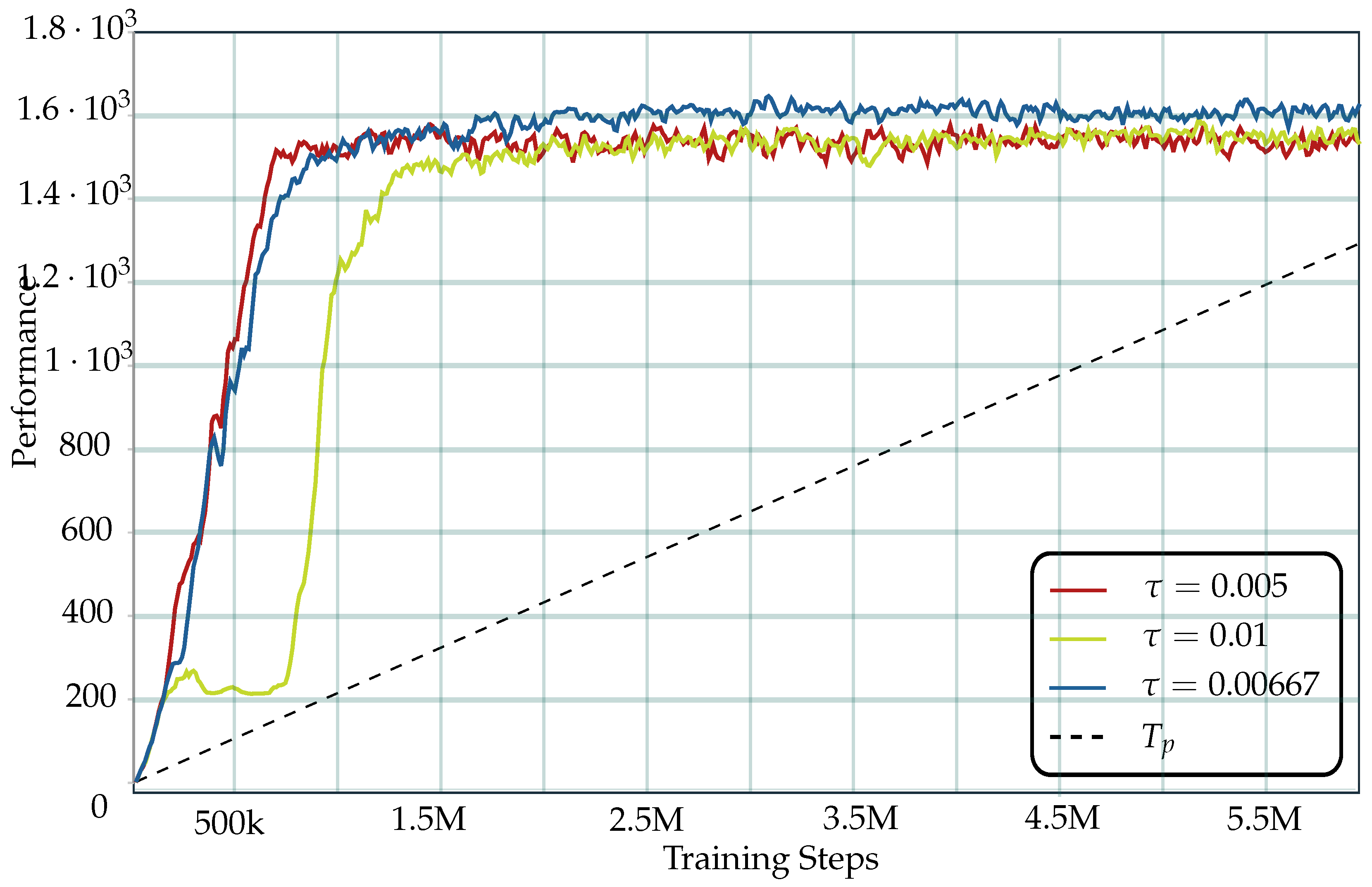
5.1. Model Configuration

The policy network is designed as an actor network with two hidden layers and a value network that also has two hidden layers, both of size 256. The hyperparameter optimization was carried out using the optuna optimizer [33]. We set the clipping parameter to  0.2  and the discount factor  γ  to  966 × 10 3 . In order to avoid major updates in the network at the end, we introduced a linear scheduler for the learning rate which decays from  1 × 10 4  to  1 × 10 8 . The policy update step is set based on the size of the problem. This parameter is sensitive towards the number of steps taken to solve the environment which is dependent on the size of the problem. For example, in the  15 × 15  instance, it was set to 448. Finally, we developed a roll out parameter for the environment which is also dependent on the problem size which helps to reduce the training time. The roll out parameter indicates when to terminate the current training phase.

5.2. Training

Training without considering OSM was carried out for each specified instance. Training with OSM was only done for a single instance of a each problem size to then determine the agent’s performance on instances of the same size. The efficiency of the solution is analyzed by using the previously obtained upper bounds for these instances. Additionally, to analyze the performance of the agent, the environment provides an occupancy cumulative average value for the job assignments. Through this, we were also able to speed up the training process by setting an occupancy threshold value which needs to be satisfied by the agent to achieve its goal, if it doesn’t, the environment terminates. By implementing this technique, the network was able to converge quicker and required less training time to reach an efficient solution. Training was stopped when the agent’s cumulative discounted reward ceased to improve. The most successful model from the training phase was employed to determine the final make span.

5.3. Benchmark Instances

To evaluate the performance, we have used the commonly used benchmark instances in this field of study. Table 1 and Table 2 present an overview of the instances that were used for training and evaluation. We mainly compared our performance using Taillard [10] and Demirkol et al. [11] instances with Han and Yang [25], Zhang et al. [2] and Tassel et al. [26], as they used same benchmark instances. For our generalized approach, we compare our results with Zhang et al. [2], even though we are not size agnostic, we achieved partial generalization in terms of problem size.

5.4. Results

We compare our results with the existing state-of-the-art algorithms and with common heuristics. Table 2 provides an overview of the corresponding performances. The agent was able to perform better for small size instances and achieved comparable performance for large scale instances. Even though the agent was not able to perform better than the state-of-the-art DRL approach by Tassel et al. [26], the goal of this study was to develop a generalized agent which could achieve a good performance without having trained on an instance of the same size.

5.5. Generalized Result

Based on the generalization research, Zhang et al. [2]’s approach using graph neural networks has produced promising results. The training time for larger instances is drastically reduced using their size-agnostic network. Although we are not size agnostic, we developed our generalization approach with respect to the problem size. Through this approach, we were able to produce better results with reduced execution time since the training is necessary only once with a particular problem size. We have compared our results based on different problem sizes with Taillard [10] and Demirkol et al. [11]. We tried three different execution rates  τ = 0.01 τ = 0.00667 τ = 0.005  which impose 15%, 10%, 5% swaps in the original  15 × 15  dataset, while 10%, 7.5%, 5% for the  30 × 20  dataset.
For the problem size  15 × 15 , the agent was trained with Taillard’s 01 and tested with other  15 × 15  instances of Taillard’s. It can be clearly observed from Table 3, Table 4 and Table 5 that, with constrained randomness, the agent was able to generalize better and produce near optimum solutions.
The agent’s performance in the environment without OSM is better than its performance in a OSM-environment. However the training time required to train 10 instances of the same size is reduced by a factor of 10 when using the OSM-environment. This is due to the fact that the training results of the first instance can be transferred to the remaining nine instances.

6. Conclusions

In this paper, we have developed a reinforcement learning environment that solves JSSPs. Moreover we showed the increased generalization capability when employing our OSM implementation. The main motive of our work was to develop a generalized model that can provide near optimum solutions. Even though, our approach is not fully generalized like Zhang et al. [2] we provide a size dependent generalization which is of high relevance for the industry. Based on the generalized result, it is clear that our approach outperforms the Priority Dispatching Rule based DRL approach by Zhang et al. [2]. Based on single instance training, our results show that our agent performed similarly to the state of the art DRL algorithms. For our future work, we plan to modify this approach to be size-agnostic which can be used by the industry to obtain more reliable scheduling results.

Author Contributions

Conceptualization, P.K., D.V. and N.K.; methodology, D.V., S.W. and N.K.; software, P.K., D.V. and S.W.; validation, P.K., D.V. and S.W.; formal analysis, D.V.; writing, all authors; supervision, N.K.; project administration, N.K.; All authors have read and agreed to the published version of the manuscript.

Funding

This project is supported by the Federal Ministry for Economic Affairs and Climate Action (BMWK) on the basis of a decision by the German Bundestag (KK5213903LB1).

Data Availability Statement

Not applicable.

Conflicts of Interest

The authors declare no conflict of interest.

Abbreviations

The following abbreviations are used in this manuscript:
COPCombinatorial Optimization Problem
DRLDeep Reinforcement Learning
JSSPJob Shop Scheduling Problem
LBLower Bound
MDPMarkov Decision Process
OSMOrder Swapping Mechanism
PPOProximal Policy Optimization

References

  1. Pinedo, M.L. Scheduling; Springer: New York, NY, USA, 2012; pp. 183–215. [Google Scholar]
  2. Zhang, C.; Song, W.; Cao, Z.; Zhang, J.; Tan, P.S.; Chi, X. Learning to dispatch for job shop scheduling via deep reinforcement learning. Adv. Neural Inf. Process. Syst. 2020, 33, 1621–1632. [Google Scholar]
  3. Sutton, R.S.; Barto, A.G. Reinforcement Learning: An Introduction; MIT Press: Cambridge, MA, USA, 2018. [Google Scholar]
  4. Silver, D.; Hubert, T.; Schrittwieser, J.; Antonoglou, I.; Lai, M.; Guez, A.; Lanctot, M.; Sifre, L.; Kumaran, D.; Graepel, T.; et al. Mastering chess and shogi by self-play with a general reinforcement learning algorithm. arXiv 2017, arXiv:1712.01815. [Google Scholar]
  5. Vinyals, O.; Babuschkin, I.; Czarnecki, W.M.; Mathieu, M.; Dudzik, A.; Chung, J.; Choi, D.H.; Powell, R.; Ewalds, T.; Georgiev, P.; et al. Grandmaster level in StarCraft II using multi-agent reinforcement learning. Nature 2019, 575, 350–354. [Google Scholar] [CrossRef] [PubMed]
  6. Du, H.; Yan, Z.; Xiang, Q.; Zhan, Q. Vulcan: Solving the Steiner Tree Problem with Graph Neural Networks and Deep Reinforcement Learning. arXiv 2021, arXiv:2111.10810. [Google Scholar]
  7. Afshar, R.R.; Zhang, Y.; Firat, M.; Kaymak, U. A state aggregation approach for solving knapsack problem with deep reinforcement learning. In Proceedings of the Asian Conference on Machine Learning, PMLR, Bangkok, Thailand, 18–20 November 2020; pp. 81–96. [Google Scholar]
  8. Manerba, D.; Li, Y.; Fadda, E.; Terzo, O.; Tadei, R. Reinforcement Learning Algorithms for Online Single-Machine Scheduling. In Proceedings of the 2020 15th Conference on Computer Science and Information Systems (FedCSIS), Sofia, Bulgaria, 6–9 September 2020. [Google Scholar] [CrossRef]
  9. Li, Y.; Carabelli, S.; Fadda, E.; Manerba, D.; Tadei, R.; Terzo, O. Machine learning and optimization for production rescheduling in Industry 4.0. Int. J. Adv. Manuf. Technol. 2020, 110, 2445–2463. [Google Scholar] [CrossRef]
  10. Taillard, E. Benchmarks for basic scheduling problems. Eur. J. Oper. Res. 1993, 64, 278–285. [Google Scholar] [CrossRef]
  11. Demirkol, E.; Mehta, S.; Uzsoy, R. Benchmarks for shop scheduling problems. Eur. J. Oper. Res. 1998, 109, 137–141. [Google Scholar] [CrossRef]
  12. Schulman, J.; Wolski, F.; Dhariwal, P.; Radford, A.; Klimov, O. Proximal policy optimization algorithms. arXiv 2017, arXiv:1707.06347. [Google Scholar]
  13. Taillard, E.D. Parallel taboo search techniques for the job shop scheduling problem. ORSA J. Comput. 1994, 6, 108–117. [Google Scholar] [CrossRef]
  14. Van Laarhoven, P.J.; Aarts, E.H.; Lenstra, J.K. Job shop scheduling by simulated annealing. Oper. Res. 1992, 40, 113–125. [Google Scholar] [CrossRef]
  15. Pezzella, F.; Morganti, G.; Ciaschetti, G. A genetic algorithm for the flexible job-shop scheduling problem. Comput. Oper. Res. 2008, 35, 3202–3212. [Google Scholar] [CrossRef]
  16. Cappart, Q.; Moisan, T.; Rousseau, L.M.; Prémont-Schwarz, I.; Cire, A.A. Combining reinforcement learning and constraint programming for combinatorial optimization. In Proceedings of the AAAI Conference on Artificial Intelligence, virtually, 2–9 February 2021; Volume 35, pp. 3677–3687. [Google Scholar]
  17. Oren, J.; Ross, C.; Lefarov, M.; Richter, F.; Taitler, A.; Feldman, Z.; Di Castro, D.; Daniel, C. SOLO: Search online, learn offline for combinatorial optimization problems. In Proceedings of the International Symposium on Combinatorial Search, Guangzhou, China, 26–30 July 2021; Volume 12, pp. 97–105. [Google Scholar]
  18. Zhang, Z.; Liu, H.; Zhou, M.; Wang, J. Solving dynamic traveling salesman problems with deep reinforcement learning. IEEE Trans. Neural Netw. Learn. Syst. 2021, 34, 2119–2132. [Google Scholar] [CrossRef]
  19. d O Costa, P.R.; Rhuggenaath, J.; Zhang, Y.; Akcay, A. Learning 2-opt heuristics for the traveling salesman problem via deep reinforcement learning. In Proceedings of the Asian Conference on Machine Learning, Bangkok, Thailand, 18–20 November 2020; pp. 465–480. [Google Scholar]
  20. Zhang, R.; Prokhorchuk, A.; Dauwels, J. Deep reinforcement learning for traveling salesman problem with time windows and rejections. In Proceedings of the 2020 International Joint Conference on Neural Networks (IJCNN), Glasgow, UK, 19–24 July 2020; pp. 1–8. [Google Scholar]
  21. Zhang, W.; Dietterich, T.G. A reinforcement learning approach to job-shop scheduling. IJCAI 1995, 95, 1114–1120. [Google Scholar]
  22. Deale, M.; Yvanovich, M.; Schnitzuius, D.; Kautz, D.; Carpenter, M.; Zweben, M.; Davis, G.; Daun, B. The space shuttle ground processing scheduling system. Intell. Sched. 1994, 423–449. [Google Scholar]
  23. Gabel, T.; Riedmiller, M. Distributed policy search reinforcement learning for job-shop scheduling tasks. Int. J. Prod. Res. 2012, 50, 41–61. [Google Scholar] [CrossRef]
  24. Liu, C.L.; Chang, C.C.; Tseng, C.J. Actor-critic deep reinforcement learning for solving job shop scheduling problems. IEEE Access 2020, 8, 71752–71762. [Google Scholar] [CrossRef]
  25. Han, B.A.; Yang, J.J. Research on adaptive job shop scheduling problems based on dueling double DQN. IEEE Access 2020, 8, 186474–186495. [Google Scholar] [CrossRef]
  26. Tassel, P.; Gebser, M.; Schekotihin, K. A reinforcement learning environment for job-shop scheduling. arXiv 2021, arXiv:2104.03760. [Google Scholar]
  27. Błażewicz, J.; Ecker, K.H.; Pesch, E.; Schmidt, G.; Weglarz, J. Scheduling Computer and Manufacturing Processes; Springer Science & Business Media: Cham, Switzerland, 2001; pp. 273–315. [Google Scholar]
  28. Mohtasib, A.; Neumann, G.; Cuayáhuitl, H. A study on dense and sparse (visual) rewards in robot policy learning. In Proceedings of the Annual Conference towards Autonomous Robotic Systems; Springer: Cham, Switzerland, 2021; pp. 3–13. [Google Scholar]
  29. Singh, S.; Cohn, D. How to dynamically merge Markov decision processes. In Proceedings of the 1997 Conference on Advances in Neural Information Processing Systems; MIT Press: Cambridge, MA, USA, 1997; p. 10. [Google Scholar]
  30. Zhang, T.; Xie, S.; Rose, O. Real-time job shop scheduling based on simulation and Markov decision processes. In Proceedings of the 2017 Winter Simulation Conference (WSC), Las Vegas, NV, USA, 3–6 December 2017; pp. 3899–3907. [Google Scholar]
  31. Brockman, G.; Cheung, V.; Pettersson, L.; Schneider, J.; Schulman, J.; Tang, J.; Zaremba, W. Openai gym. arXiv 2016, arXiv:1606.01540. [Google Scholar]
  32. Raffin, A.; Hill, A.; Gleave, A.; Kanervisto, A.; Ernestus, M.; Dormann, N. Stable-baselines3: Reliable reinforcement learning implementations. J. Mach. Learn. Res. 2021, 22, 12348–12355. [Google Scholar]
  33. Akiba, T.; Sano, S.; Yanase, T.; Ohta, T.; Koyama, M. Optuna: A Next-generation Hyperparameter Optimization Framework. arXiv 2019, arXiv:1907.10902. [Google Scholar]
  34. Adams, J.; Balas, E.; Zawack, D. The shifting bottleneck procedure for job shop scheduling. Manag. Sci. 1988, 34, 391–401. [Google Scholar] [CrossRef]
  35. Fisher, H. Probabilistic learning combinations of local job-shop scheduling rules. Ind. Sched. 1963, 225–251. [Google Scholar]
  36. Lawrence, S. Resouce Constrained Project Scheduling: An Experimental Investigation of Heuristic Scheduling Techniques (Supplement); Graduate School of Industrial Administration, Carnegie-Mellon University: Pittsburgh, PA, USA, 1984. [Google Scholar]
  37. Applegate, D.; Cook, W. A computational study of the job-shop scheduling problem. ORSA J. Comput. 1991, 3, 149–156. [Google Scholar] [CrossRef]
  38. Yamada, T.; Nakano, R. A genetic algorithm applicable to large-scale job-shop problems. In Proceedings of the Second Conference on Parallel Problem Solving from Nature, Brussels, Belguim, 28–30 September 1992; pp. 281–290. [Google Scholar]
  39. Storer, R.; Wu, S.; Vaccari, R. New search spaces for sequencing instances with application to job shop. Manag. Sci. 1992, 38, 1495–1509. [Google Scholar] [CrossRef]
Figure 1. Job sequence on machines for a job shop problem with 3 machines and 2 jobs.
Make 05 00025 g001
Figure 2. Comparison between the environment with the OSM implementation (red) and environment without the OSM (blue)—performance of the agent vs. training steps.
Make 05 00025 g002
Figure 3. Comparison between the environment with the OSM implementation (red) and environment without the OSM (blue)—episode length vs. training steps.
Make 05 00025 g003
Figure 4. Performance with different execution rates—agent performance vs. time steps  ( green : τ = 0.01 ,   blue : τ = 0.00667 ,   red : τ = 0.005 ,   black T p ) .
Make 05 00025 g004
Figure 5. Performance with different execution rates—episode length vs. training steps  ( green : τ = 0.01 ,   blue : τ = 0.00667 ,   red : τ = 0.005 .
Make 05 00025 g005
Table 1. Benchmark instances.
AuthorsInstance Size Used (Jobs × Machines)
Adams, Balas, and Zawack [34]10 × 10, 20 × 15
Demirkol, Mehta, and Uzsoy [11]20 × 15 to 50 × 20
Fisher [35]6 × 6, 10 × 10, 20 × 5
Lawrence [36]10 × 10 to 15 × 5
Applegate and Cook [37]10 × 10
Taillard [10]15 × 15 to 20 × 100
Yamada and Nakano [38]20 × 20
Storer, Wu, and Vaccari [39]20 × 10 to 50 × 10
Table 2. Performance comparison of the conventional env model, * indicates the solution is optimal.
InstanceSize (n × m)MWKRSPTTassel et al. [26]Han and Yang [25]Zhang et al. [2]OursLB
Ft066 × 6-----55 *55
La0510 × 5787827-593 *-593 *593
La1015 × 511361345-958 *-958 *958
La1610 × 1012381588-980-974945
Ta0115 × 1517861872-1315144313521231
Ta0215 × 1519441709-1336154413541244
dmu16 [11]30 × 205837624141884414495346323751
dmu17 [11]30 × 20661064874274-557951043814
Ta4130 × 202632306722082450266725832005
Ta4230 × 202401364021682351266424571937
Ta4330 × 20316228432086-243124221846
Table 3. Generalized Taillard’s  15 × 15  instance results with various OSM execution rate.
InstanceTa01-OSM with 5%Ta01-OSM with 10%Ta01-OSM with 15%MWKRSPTOursZhang et al. [2]LB
Ta0214911486154619441709135415441244
Ta0314431437152519472009138814401218
Ta0415681502161416941825151316371175
Ta0515991481148318922044144316191224
Ta0617761507155219761771136016011238
Ta0715261500160519612016135415681227
Ta0816311540152418031654137714681217
Ta0916621664159722151962140116271274
Ta1015731524165920572164137015271241
Table 4. Generalized Taillard’s  30 × 20  instance results with various OSM.
InstanceTa41-OSM with 5%Ta41-OSM with 7.5%Ta41-OSM with 10%MWKRSPTOursZhang et al. [2]LB
Ta4229032831257233943640245726641937
Ta4328002651261431622843242224311846
Ta4429912751274533883281259827141979
Ta4528512812269233903238258726372000
Ta4629862842267432683352260627762006
Ta4728542807267729863197253824761889
Ta4827582753263830503445246124901937
Ta4928002646256631723201250125561961
Ta5028872654261629783083255026281923
Table 5. Generalized Demikrol  30 × 20  instance results with various OSM (MWKR refers to Most Work Remaining, SPT refers to Shortest Processing Time).
InstanceTa41-OSM with 5%Ta41-OSM with 7.5%Ta41-OSM with 10%MWKRSPTOursZhang et al. [2]LB
Dmu1654135560490758376241463249533751
Dmu1759265911564666106487510453793814
Dmu1853805773528763636978499851003844
Dmu1952365136499363855767475948893768
Dmu2052635318513164726910469748593710
Disclaimer/Publisher’s Note: The statements, opinions and data contained in all publications are solely those of the individual author(s) and contributor(s) and not of MDPI and/or the editor(s). MDPI and/or the editor(s) disclaim responsibility for any injury to people or property resulting from any ideas, methods, instructions or products referred to in the content.

