Article

Lottery Ticket Search on Untrained Models with Applied Lottery Sample Selection

Computer Science, University of Windsor, 401 Sunset Ave, Windsor, ON N9B 3P4, Canada
*
Author to whom correspondence should be addressed.
These authors contributed equally to this work.
Mach. Learn. Knowl. Extr. 2023, 5(2), 400-417; https://doi.org/10.3390/make5020024
Submission received: 6 March 2023 / Revised: 11 April 2023 / Accepted: 16 April 2023 / Published: 18 April 2023
(This article belongs to the Section Data)

Abstract

:
In this paper, we present a new approach to improve tabular datasets by applying the lottery ticket hypothesis to tabular neural networks. Prior approaches were required to train the original large-sized model to find these lottery tickets. In this paper we eliminate the need to train the original model and discover lottery tickets using networks a fraction of the model’s size. Moreover, we show that we can remove up to 95% of the training dataset to discover lottery tickets, while still maintaining similar accuracy. The approach uses a genetic algorithm (GA) to train candidate pruned models by encoding the nodes of the original model for selection measured by performance and weight metrics. We found that the search process does not require a large portion of the training data, but when the final pruned model is selected it can be retrained on the full dataset, even if it is often not required. We propose a lottery sample hypothesis similar to the lottery ticket hypotheses where a subsample of lottery samples of the training set can train a model with equivalent performance to the original dataset. We show that the combination of finding lottery samples alongside lottery tickets can allow for faster searches and greater accuracy.

1. Introduction

The lottery ticket hypothesis has shifted the field of pruning networks and allows us to create a standard for discovering smaller networks within larger neural network. It states that given a dense neural network that is randomly initialized, there exists a subnetwork that can match the performance of the original using at most the same number of training iterations. The weights that allow us to find such a subnetwork are ideally lottery ticket weights, which are the key weights to fit the dataset properly. The hypothesis tells us a smaller subnetwork should be possible, but often it requires us to train the original network in order to select potential lottery weights. To validate subnetworks, the subnetwork must be reinitialized to the original weights (prior to training) and retrained, thus making a redundant use of training. Moreover, the dataset itself is not optimized in any way during this process. Should a subnetwork require the entire dataset?
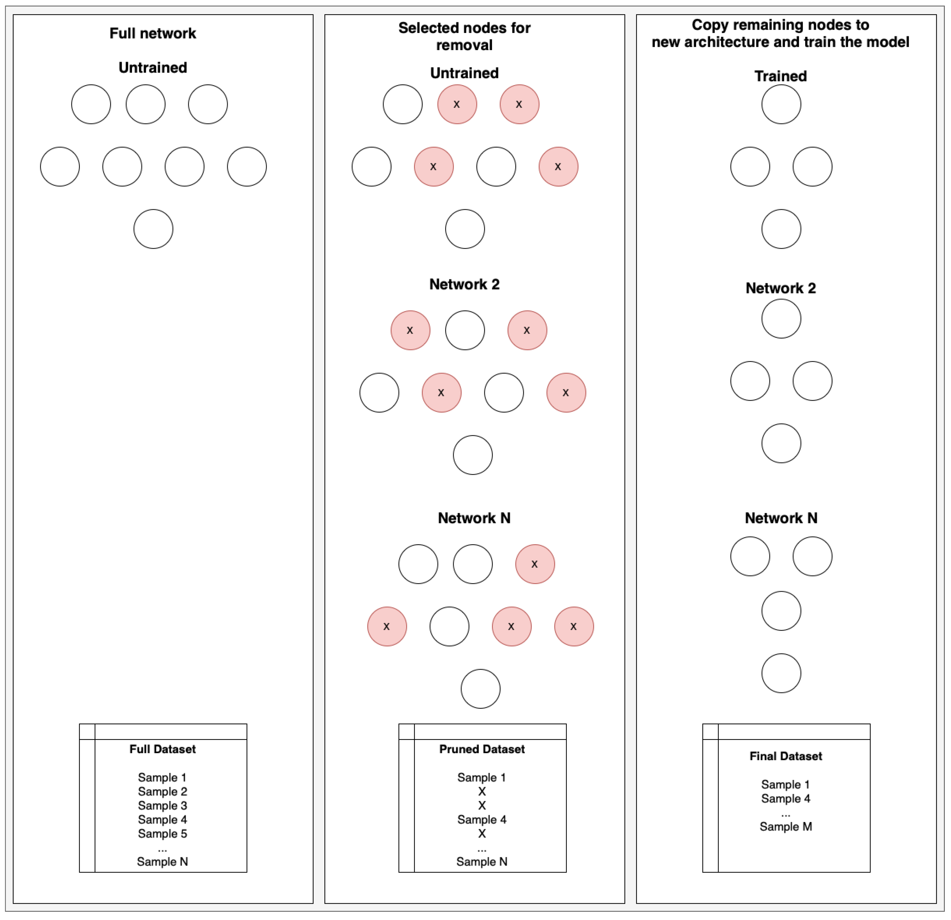
In this paper we aim to reverse how we discovery lottery tickets. We first propose an approach to search for lottery tickets without training the original model. This removes the redundancy of first training the original network, then retraining the subnetwork. Second, we propose an expansion to the lottery ticket hypothesis by applying it to the training set of the model. Given a training dataset for a network, we claim there exists a subset of samples to train the same network (or subnetwork) with equivalent performance to that achieved from the original dataset. This would allow researchers to explore the idea of applying approaches learned from lottery ticket algorithms to dataset reduction for higher quality datasets.
We apply some of these ideas to tabular neural networks on a large variety of datasets. The tabular neural network was shown to be a leading model for tabular datasets in our recent paper [1]. It has been shown to be leading in many other tabular problems [2,3,4,5]. In particular a highway study mentions “Fast.ai neural network model for tabular data: Fast.ai model has demonstrated the state-of-art performance in the tabular data modeling in this study.” [5]. And is often used to achieve state-of-the-art performance, “the FastAI tabular model was selected because it has thus far obtained the best classification result on the [Anatomical Therapeutic Chemical (ATC)] benchmark” [3]. The network design allows for categorical embedding and continuous features to be processed through a series of linear layers and optional batch normalization.
The contributions of our paper is as follows: (1) the lottery ticket search no longer limited by the size of the original model; (2) we remove the need to train the large original network (which is usually trained and tested multiple times); (3) we show that large parts of the training dataset, up to 95% reduction, is not required to find lottery tickets; (4) we show these improvements are not tradeoffs, but allow the algorithm to perform equivalently or better than prior methods at searching for lottery tickets; (5) we present an extention of the lottery ticket hypothesis to include the ability to also prune the dataset using a similar approach.
Our paper is organized as follows. First, we present previous works on the lottery ticket hypotheses, dataset reduction, tabular models, and the use of the genetic algorithm for pruning techniques. Second, we describe the datasets we use and the approach we take to prune our models using a genetic algorithm and reduce training samples. Third, we present our experiments and results of our pruning strategy. Finally, the paper is concluded including future work.

2. Previous Works

The lottery ticket hypothesis [6] has been tested on a variety of network architectures. All use a similar goal to prune a network by a large margin, usually over 80%, and have a model perform similarly or even better than the original network. For example, there have been many attempts at pruning convolutional neural networks (CNNs) which include the original paper on lottery tickets itself [6] (80–90% prune rate), a generalized approach [7] to prune across many vision datasets (such as MNIST, SVHN, CIFAR-10/100, ImageNet, and Places365), and an object detection variant [8] pruned up to 80%.
There have been many tests of the lottery ticket hypotheses applied to large pre-trained networks. In this case we have large pre-trained models which no longer have the original weights, so the test of the lottery ticket hypotheses is be performed on downstream tasks [9]. In this case they did not structurally prune the model but applied masks leading to a 40–90% sparsity depending on the downstream task. Other papers, such as [10], have proposed to structurally prune transformers using question-answering tasks and achieving double inference speeds with a minor loss of accuracy. S. Prasanna, A. Rogers, and A. Rumshisky [11] made an interesting study on good and bad subnetworks found based on the down-steam task.
We use a mix of regression and classification tasks for evaluation. Many works focus on these types of problems, for example some different areas of focus are sentiment analysis [12], malware detection [13], ensemble of models focusing on a task [14], and camera messaging systems [15,16]. Our work aims at tackling regression and classification problems in a generic set of tasks within a tabular context. Generally tabular data is processed by models like random forest (RF), k-nearest neighbors (KNN), gradient boosting (GB), etc. There are high performance deep neural networks that have been shown to perform well on tabular data such as timeseries TabBERT [17], and TabTransformer [18], both based on the natural language processing transformer model using attention [19]. We chose the FastAI network for its ability to perform given its small size in line with our goal to propose a method to produce small networks in a stable manner without training the original model, adaptable to many different datasets.
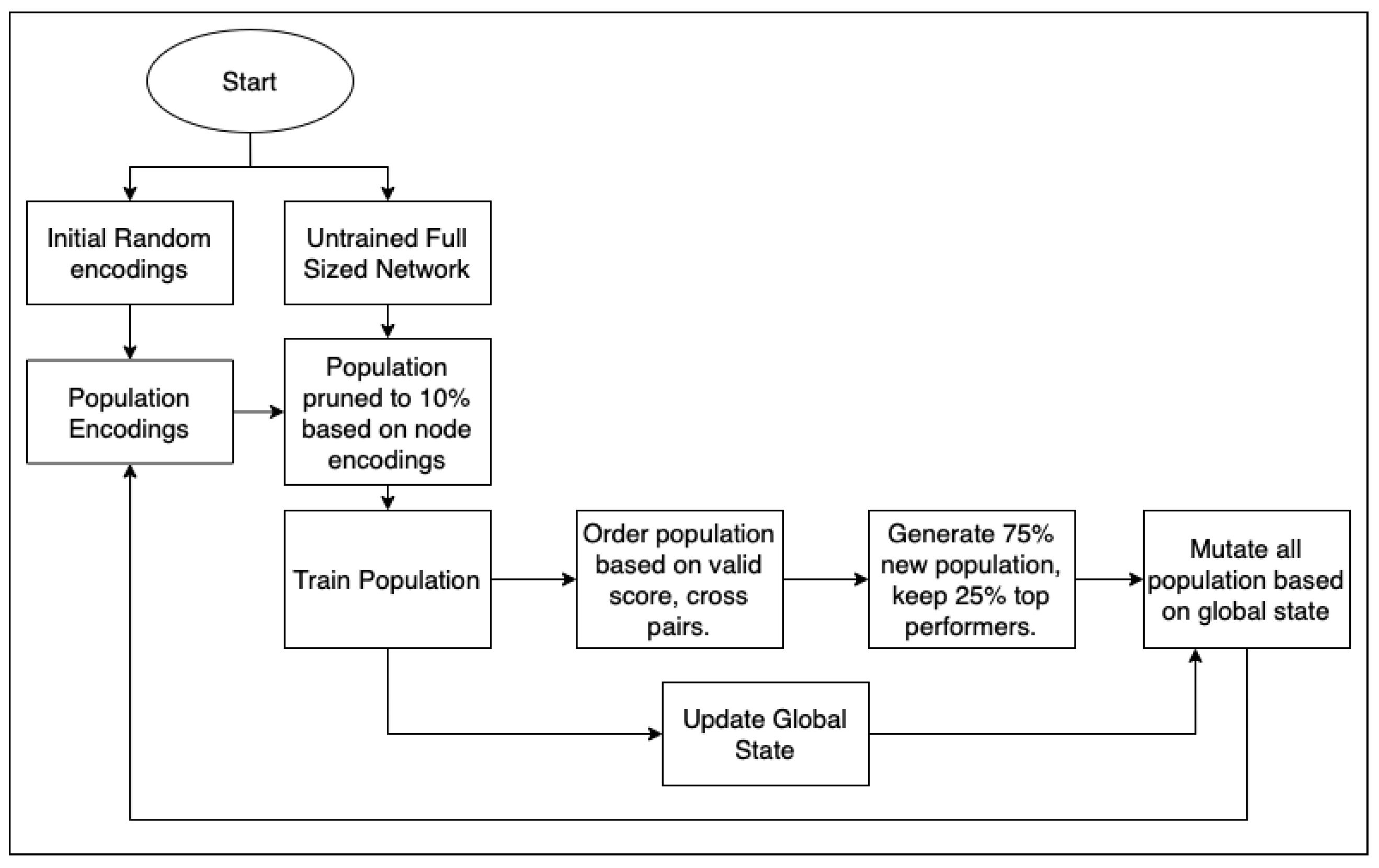
Our approach uses a genetic algorithm in order to produce small networks by pruning them through generations of subnetwork tests by fixing the size and optimizing for best accuracy, and in particular our approach aims to avoid training the original network altogether. Genetic algorithms have been used for pruning in other works. For example Z. Wang et al. [20] use a genetic algorithm to prune channels of a CNN by optimizing for size and minimizing accuracy loss at the same time. The authors directly mention “after pruning, the structure of the new network and the parameters of the reserved channels must be retrained” [20]. D. Mantzaris et al. [21] use a genetic algorithm as a feature selection approach which in turn reduces input nodes but is not directly testing the idea of lottery ticket pruning which would fix weights and search for subnetworks. C. Yang et al. [22] also prune a CNN with a two step process. “First, we prune the network by taking the advantages of swarm intelligence. Next, we retrain the elite network and reinitialize the population by the trained elite.” [22]. Note that they must “retrain the elite genome so that the remained weights can compensate for the loss of accuracy” [22]. P.J. Hancock [23] from 1992 even tested the idea of pruning a network using a genetic algorithm. The method first trains the original network, then uses the genetic algorithm to prune it, “then prunes connections prior to retraining of the remainder” [23]. We aim to eliminate the training process of the original network which also eliminates the redundancy of retraining the subnetwork. Thus instead of the typical approach, 1. train original network, 2. select sub networks, 3. retrain subnetworks independently, we instead skip step 1 and simply train instead of “retrain” the subnetwork.
There are a few other things we wanted to highlight. First the original lottery paper [6] mentions that normal pruning often leads to less accurate models, but applications of pruning in search of lottery tickets tends to resolve this issue. Second, in the generalized work on pruning CNNs [7] they mention larger datasets tend to produce better lottery tickets. Finally, in our previous work [1] we found that larger networks tend to hold more lottery tickets which made it easier to find a set of tickets when pruning. This leads us to the idea that the approach or concept of lottery tickets can be applied to datasets, like finding lottery samples. For instance, in comparison to the first point, removal of training data generally leads to less accurate models which is well known so ideally finding lottery samples could relieve this issue. In the second point larger dataset tends to produce better lottery tickets which can suggest that there was a higher chance the dataset contains key lottery samples to find better lottery tickets, much like how a larger network may contain more lottery tickets just by chance. The idea here is that samples are tied to lottery tickets, thus the set of samples that belong to a subnetwork of lottery tickets would be lottery samples. Thus we propose the idea that a subset of samples, or lottery samples, can be found and used to find lottery tickets and train a subnetwork with similar accuracy to the original larger network on the full dataset.
Much like pruning prior to the lottery ticket hypotheses, the concept of training reduction has been tested in many papers. For example, S. Ougiaroglou et al. [24] used dataset reduction in order reduce the amount of space and inference complexity KNN requires from holding the dataset for nearest neighbor comparisons. In this case it is a model specific example of how a few key samples can result in a similar model. However, KNN and similar distance based algorithms can be very inefficient and does not indicate if this reduced training dataset can be useful to other models. F.U. Nuha et al. [25] applies dataset reduction to generative adversarial networks (GANs) to show that a dataset with 50k samples is ideal and can outperform a larger noisy dataset. J. Chandrasekaran et al. [26] uses random sampling to reduce the dataset with the goal of tuning the hyperparameters of a model faster. They show that the reduction of the dataset down to 800 samples has the same coverage as the original allowing them to use the reduced dataset for model testing.
What we propose is that dataset reduction can benefit from reshaping the problem as lottery samples through a combination of sample selection and lottery ticket pruning. The pruning process would allow the network to properly fit a given dataset reduction without overfitting and allow for faster training times without complex selection algorithms. For example, we show a random subsampling is enough for us to achieve equivalent models when we use it in conjunction with lottery ticket pruning (as the tickets found fit the subset of data), allowing us to potentially reduce training datasets down to 5% their original size, some at just 13 samples. This would also open dataset reduction to techniques found by lottery ticket pruning that can be applied to sample selection problems (such as the genetic algorithm we propose for lottery ticket selection) to stabilize the reduction and improve coverage.

3. Materials and Methods

In this section we introduce the datasets used to test our lottery ticket search algorithm, then we describe the algorithm in the following subsection. The approach is split into two subsections where the methodology of our lottery ticket node pruning strategy (without training of the original network) is first described in the genetic lottery node selection subsection. In the next subsection we describe our application of lottery sample selection to our algorithm to improve the algorithm’s performance.

3.1. Datasets

The lottery ticket search algorithm is built on our previous work [1] which presented improvements in tabular neural networks using pruning strategies based on the lottery ticket hypotheses. We use the same datasets to evaluate our search algorithm, we refer to our previous work for more details on the datasets used in our evaluation. In summary, the datasets have a wide variety of tabular qualities such as many (or little) categorical and/or continuous features, missing or poor data, a range of a few hundred to millions of samples including simulated data, defined and undefined prediction goals and test sets, etc. The exact quality of each dataset can be found in our paper [1], we included this information in Appendix A. We kept the same train/valid/test split sizes as our previous paper, shown in Table A1, although the split may not contain exactly the same samples due to different randomization initializations and variations of code.
We include the following datasets in our tests: Alcohol [27], Video Games Sales (https://github.com/GregorUT/vgchartzScrape, kaggle: https://www.kaggle.com/gregorut/videogamesales, accessed on 26 September 2022), Wine Quality [28], Chocolate Ratings (https://www.kaggle.com/rtatman/chocolate-bar-ratings, accessed on 26 September 2022), Poker Hand [29], Titanic (https://www.kaggle.com/c/titanic/data, accessed on 26 September 2022), Health Insurance (https://www.kaggle.com/anmolkumar/health-insurance-cross-sell-prediction, accessed on 26 September 2022), Susy dataset [30] (see Table 1).
The datasets use RMSE or F1 as a metric which depends on the type of classification or regression task used in each dataset. For example, the health dataset is a classification task which aims to predict 1 or 0, so we use F1 as a metric. On the other hand we have continuous tasks which is ideally measured with regression metrics such as RMSE, like the video game dataset focused on sales. The details on all datasets and tasks are provided in Appendix A. Some datasets could use either metric, RMSE or F1, but these are mainly decided in our previous work and thus kept the same for this work for comparison purposes.

3.2. Methodology Overview

Our method is a general machine learning approach to train a small but accurate neural network. Our method is applied to a larger untrained model where it selects as little as 10% of nodes to be tested. The still-untrained nodes, once selected, will be copied to a smaller neural network architecture. From there we apply a random dataset selection which can reduce the amount of data to process by up to 95%. Together, these two pieces allow us to fully evaluate the smaller neural network efficiently to search the node space in our proposed approach. See the diagram of this prune process in Figure 1.
In this section we present our proposed approach in two subsections. The purpose of the algorithm is to improve model pruning based on the lottery ticket hypotheses, which is described in the first subsection. As a result of improving model pruning, we find a smaller equivalent (or better) model. Our approach uses a genetic algorithm (GA) to search for lottery tickets which allows us to prune non-lottery ticket nodes. Throughout generations of the GA we search for pruned models maintaining the original accuracy of the larger model. The approach contributes a design that does not require training of the original network, thus saving on computations with a scalable design. Other approaches like iterative pruning would require training of a large network several times over (iteratively), repeated for each test.
The next subsection we improvement on our approach by applying an extention to the lottery ticket hypotheses that we propose. This extension states we don’t need the full dataset to search for lottery tickets, meaning we can find a smaller equivalent model using a fraction of the training data. This method applies random selection of the training data in conjunction with lottery ticket pruning to show that lottery samples exist. These lottery samples save on training requirements by removing up to 95% of the original dataset, thus allowing us to efficiently search for pruned models.

3.2.1. Genetic Lottery Node Selection

We recreated the FastAI [31] tabular neural network in order to build a prune strategy on top of it based on the lottery ticket hypothesis. The network consists of embeddings to process categorical features which are then appended to the set of continuous features. This layer is processed through a series of linear layers with optional batch normalization at each stage. Since our goal is to reduce network size, we eliminated all batch normalization layers, but we also have tested with batch normalization which did not perform as well for smaller networks [1]. We apply some preprocessing to the datasets which include converting categorical features to IDs for embeddings, filling in missing data, and normalizing continuous features. The training strategy used increases and lowers the learning rate in cycles to reach a better local minima of the loss function. We perform early stopping on the best validation score for a fixed number of training cycles.
We outline the general structure of the approach in Figure 2. The goal of our approach is to find a pruned network as performant as the original network without having to train the original network. Our previous approach would require the original network trained in order to measure the weights and generate a metric to prune them. With our current approach we do not need to train the original network, although we do in this paper for comparison purposes to validate the approach. This would allow the option to create a large search area for lottery tickets without the consequence of having to train the large network. To avoid training the original network, we pre-prune the network using a genetic algorithm (GA) approach. The genetic algorithm requires a population, and a means to evaluate the population to select and produce the next generation of individuals.
The population is a list of encodings which describe which node of the network to retain or prune. The encoding is a sequence of 1s and 0s ordered with the nodes of the (original) network to represent their prune status. We can fix the number of retained nodes in the search algorithm, which we have determined to be optimal around 10% in our tests, or 90% prune rate. The population size per generation was fixed to 30 for large datasets, and 60 for smaller datasets, selected for how much we can process on a 2-cpu machine as a criteria. Some of the small datasets of a few hundred samples could likely handle larger populations but we wanted to keep the size roughly fixed across all tests.
The initial population is randomly generated with the fixed prune rate. The population is evaluated by training the subnetworks and recording their validation scores (the test scores are not used). We then use a weight measure to score the weights of the subnetworks (see Appendix B). This measure can be norms as typically done with pruning, or can be custom metrics such as weight mean and variance, or can be a global network metric such as the validation score from evaluation. We tested many different measures in our experiments, including combinations, but overall found that the simplest metrics L0 to be one of the best performers on average for all datasets.
When the weights are measured, they are recorded into a global prune state matrix where each node (ordered by its position in the original network) has a representative entry in the global state. The global prune state is maintained throughout all generations to grow a map of knowledge regarding node quality. We provided an example of how the global state is used and updated along with the overall crossover, adjustment, and mutation process of individuals in Figure 3. Each subnetwork will contribute its node weight scores to their respective global state entry (using the mean of multiple scores if different population overlap in nodes). The quality scores in the global state are normalized to a value between 1 and 0, 1 being the best quality measurable. Since the nodes are initially untested, they start with a full quality score of 1. The quality scores are normalized to probabilities when used to mutate or select nodes during the crossing processes.
We reorder the individuals with a random selection weighted by normalizing their validation score, then pair them in that order. At this point we no longer need the network itself and work with the node encoding. The encoding is a sequence of 1/0s representing which nodes have been selected for the subnetwork, 0 being pruned. First, we cross the encoding pairs at K random points in the encoding. This crossover may result in an imbalance of nodes with more or less than the fixed requirement. Note that for all random node selections we use a weighted random selection using the global state’s normalized quality scores (used as probabilities). Given more nodes, we remove selected nodes at random. Otherwise, we randomly select new nodes to introduce into the individual. Then each new individual will have a series of mutations by pruning a random node and reselecting a pruned node to maintain node balance. The choice of node is random for selecting new nodes, but when removing selected nodes the random selection is weighted to weaker nodes by inverting the quality scores and normalizing for probabilities again. This process first allows generations to build off high performant networks using a cross of their encodings, then mutate them towards a potentially better selection of nodes and/or untested nodes.
We found through parameter adjustments that retaining 25% of the top performing networks of the current generation benefitted the selection process for the next generation. Note that 75% of the next generation will be newly generated population while 25% is top performers, all of which get mutated. To save time, if the same network/encoding ever reoccurs, we use their recorded score rather than retraining the network. This can happen if the original network is small or if only a few high quality nodes are available to select, thus the algorithm may converge towards similar networks. Moreover, we retain 25% of top performers with mutations applied which can reappear as they mutate to similar nodes each generation, so we see most of these top performers reoccur. For example, the alcohol dataset had about 26% of networks reoccur (over 40 generations), largely from the retained top performers, thus we save a lot of time using a simple dictionary lookup (where the key is the encoding). We used a fixed 40 generations for all our tests, then use the best model of the final generation as our pruned model. In our results we show that the fixed 40 generations can be reduced in general if we optimize globally across all datasets, and reduced even more if optimized per dataset. At no point is it required to train the original network.

3.2.2. Lottery Sample Selection

The genetic algorithm we proposed to find lottery nodes requires training of many small networks (compared to the potentially large original network). While the networks are small in size, the dataset used for training can still impose inefficient search times, for example when training on the Susy dataset with 5 million samples. To solve this problem we propose an extension to the lottery ticket hypothesis which states that not only can a subnetwork be found as performant as the original, but a subset of the training dataset (lottery samples) in conjunction with a subnetwork of lottery weights (found and trained using the subset) can be as performant as the original network using the original dataset. The validation and test sets remain the same, but the training dataset can be searched for lottery samples and used to train a model with equivalent performance, and in some cases better performing networks due to outlier and poor sample quality removal.
We found simply reducing the training dataset does not produce equivalent performance. It was required to first reduce the dataset, then find appropriate lottery weights for this dataset. We believe that the reduced dataset becomes simplified, thus requiring a simpler network to generalize the data better (using quality lottery weights). In this case we extended our genetic algorithm to first reduce the training dataset at random to a fraction of its size, then run the lottery node search for this reduced dataset. This allowed us to reduce search time for the algorithm directly proportional to the reduction in training data. We run tests with 25% to 95% reduction.

4. Experimentations, Results, and Discussion

In our previous paper we had already performed parameter searches regarding model training such as number of neurons, layers, learning rate, etc. We built on these parameters and continued to test our approach for the lottery pruning parameters specifically. Many of the parameters were tested in a grid-style approach. For example, the retained population parameter was searched in a range of 0–25 which was limited to 25 since we wanted a diverse population. The number of generations were set higher than the optimal value since we can fully exaust the performance of the genetic algorithm without loss of accuracy due to the retained population. From there we analysed the generational validation performance to determine the best stopping point in individual datasets and across all datasets. The number of subnetworks were limited by our hardware which was a 2-CPU machine, mainly to show that we can achieve great performance on low hardware requirements. Our previous paper, previous works, and in our own tests have found 80–95% prune rates to work well, so we have tested in this range. We performed a grid search on the dataset reduction testing 0%, 25%, 50%, 75%, 90%, and 95% dataset reduction. Finally we test a wide variety of pruning metrics which measure the quality of the nodes pruned.
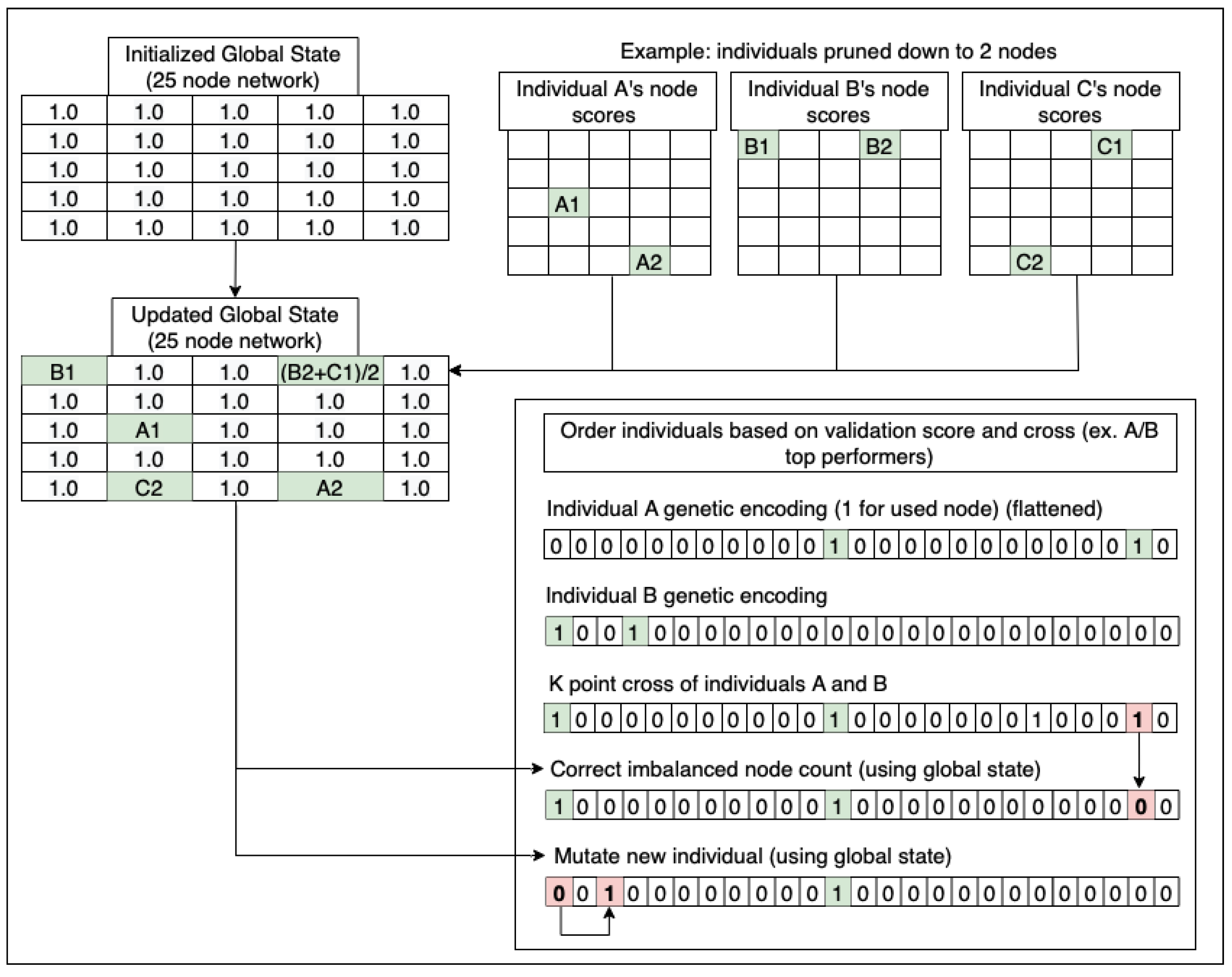
After parameter searches for the genetic algorithm, we found 25% retained population at each generation to be ideal. We chose a fixed 40 generations for all tests, but early stopping can be applied if validation performance slows or does not improve. We used 30 subnetworks per generation for large datasets, and 60 for small datasets. Population size was chosen to optimize search times on two CPUs, although with more hardware performance a higher search area can be used with more networks. We found across all datasets about 90% node reduction was optimal, so we fixed this prune rate for all our tests. We used dataset reduction as a variable search between 25–95%. The node selection measure was tested using many different norms, weight metrics, and training metrics as described in our methodology.
Our approach for lottery ticket pruning and sample selection is tested across many trials. We present results categorized by the prune method, each tested across many same reductions. The first method uses the best performing norm in our tests, L0, to measure the quality of nodes and is used across all datasets. The next test shows that a combination of norms and metrics (L0, L1, Linf, and random noise) can improve the results of our lottery ticket search further. Finally, we show that focusing on selecting the proper norm and metrics for individual datasets can lead to even greater performance. We also push the approach to its limit and describe some results of lottery ticket pruning with extreme dataset reduction.
For the first test, Table 2 highlights our best scores using the norm L0 as a single measure across all datasets. In general, it was shown to find better performing networks on 5 of 8 datasets up to 30%+ improvement. We note a loss of accuracy by 1.2% in Chocolate, 3.1% in Poker and 6.1% in Wine. In particular, it is not a surprise that the Wine dataset has poor performance since it has been shown to be resistant to lottery ticket strategies in our tests from our previous paper [1] We could not find a weight reduction of any size to improve its performance.
For the second test, Table 3 highlights our best scores using multiple norms and measures across all datasets. We simply tried random combinations of the individual measures used in an attempt to find a better pruned subnetwork. In this case we found the combination of L0, L1, Linf, and some random noise allowed the genetic algorithm to find roughly equivalent subnetworks in all but the Wine dataset, however the Wine dataset compared to L0 selection was improved marginally as well. If we think logically about the score combination used, the L1 norm is the sum of all weights, L0 is the number of non-zero weights, and Linf is the largest element. Thus, the score of their combination is looking for nodes with dense information in an attempt to reduce empty space with zero-weight counting and small-weight sums. This is likely why L0 outperformed as an individual score as it simply looks for the densest nodes of the network, but adding weight sums with L1 can help differentiate ties when density is maxed out.
The previous two tables presented results where the same measures were used on all datasets, however optimizing each dataset individually can improve results further. For the third test, Table 4 presents the best measure found for each dataset individually. The Wine dataset had a loss of accuracy of 1.6% which is only marginally worse than original. We therefore argue in every dataset we found a nearly equivalent subnetwork using a subset of the training data.
We include a graph of the validation improvement over the 40 generations for the GA algorithms of Table 4 in Figure 4. The improvement is in percentage (shown as a log chart for visibility) compared to the first generation, so all datasets start at 0% improvement and we show how the algorithm progresses over each generation. The chart shows in some cases, such as Poker, Wine and Alcohol, the full 40 generations continue to improve validation scores. For the other datasets, we find that the improvement flattens early on suggesting an early stop can be implemented for some datasets. In many datasets we could stop at generation 15, and in some even at 7 generations. Across all datasets, after 25 generations there is little performance gain, but still improvements. This would mean an early stop mechanism could be implemented to stop the search process early on and improve search times by an additional 35–80%.
We wanted to highlight some extreme cases of sample reduction on a few tests. For our large datasets, the Susy dataset had a reduction of training data by 90% (from 4M training samples to 400k) while improving F1 by 0.35%. For our smaller datasets, the Chocolate dataset was able to be reduced by 95% (from 1149 training samples to just 57 samples) while improving RMSE by 4.94%. The Alcohol dataset was reduced to 190 samples and still outperformed original by 6.71%. The Titanic dataset used 347 samples to outperform original by 5.59%. If the goal were simply to reduce training data and maintain at most equivalent performance, many of these datasets could be reduced even further with a small drop in accuracy. For example, Susy with a 95% reduction can still achieve a loss of accuracy of only 0.10% (using the same measure), while samples are reduced to 200k. In an extreme case, Alcohol had a loss of only 1.76% at 95% reduction, which corresponds to only 13 training samples. We include some network training and inference time results in Table 5. Note that inference time can be subject to CPU processing noise due to the small nature of the datasets, so we included in bold the result from the larger datasets which show improved inference.
In addition to our comparison to original (which has no dataset reduction and no weight reduction), the results in each table are compared to the original network trained with dataset reduction (equivalently reduced train dataset to the respective GA result), and random pruning (equivalent 90% prune rate) tested both with and without dataset reduction. For original trained on dataset reduction, we found it mostly made performance significantly worse, and in some cases untrainable if the reduction was too high. This is expected since generally reducing training data for neural networks tends to lead to worse performance and a reduced ability to generalize. We also found that random pruning (on the full dataset) is not enough to find lottery ticket weights and that our GA algorithm generally improves over random pruning. And finally, combining the two using random pruning and dataset reduction made performance even worse, likely compounding the overall negative effects of both. Thus, our results suggest that in order to use dataset reduction, or in other words apply the idea of lottery samples, the network must also be pruned to its lottery weights, meaning the two approaches to find lottery samples and lottery weights must work together to find an optimized subnetwork. We believe this needs to be the case because the lottery ticket weights allow the network to learn on the reduced dataset with increased generalizability allowing us to avoid overfitting the networks. The lottery weights are directly tied to the lottery samples which would imply a different selection of training samples would be tied to a different subset of optimal lottery weights.
Finally, we compare with the current leading approach on tabular datasets [1] for tabular datasets in Table 6. The first two columns are from the previous work using the best of iterative pruning or oneshot pruning algorithm. The algorithms prune starting from a model as large as [1600, 800] neurons in size (size of each linear tabular layer). The standard iterative approach (approach 1) prunes by 50% at each step until it reaches a final size of [1, 1] and use the best performing size reduction. The adaptive iterative approach (approach 2) first looks for an optimal original network size (which can vary weights), then prunes iteratively on this better network. The oneshot approach will prune directly to a size of [1, 1] which has only succeeded in the case of Alcohol. The second column is our GA working with a fixed prune rate of 90%. In this case we start with a model of size [200, 100] and prune down to 30 neurons total. The comparison shown is the improvement over the original starting network of the respective model that was pruned, so this score is based on the starting network used.
We do not compare best accuracy in this case because this depends on the original model (which can change with varying sizes, better initialization of lottery weights, and/or training strategy) and the goal of the paper is to create an algorithm to improve the search method to find lottery tickets. In some datasets for the previous approach, the best model could only be found with hundreds of neurons while we can still achieve similar improvements on small networks. We show that our approach generally finds lottery tickets and improves over the original starting network in most datasets, and show the benefit of a fixed prune rate to achieve a fixed final size of the network. We also want to highlight that our GA approach never trains the original network while still being able to compete with and outperform the current leading approach that requires training and retraining of the subnetwork several times over on an iterative scheme. In addition, we only use a fraction of the training dataset in the GA approach.

5. Conclusions and Future Work

In conclusion, we designed a genetic algorithm capable of searching for lottery tickets using a fraction of the training dataset without ever training the original network. The algorithm can target a fixed prune rate and search for lottery tickets by training networks a fraction of the size of the original network. We were able to find networks 90% smaller than original while improving up to 30% in accuracy in some cases. We demonstrated that the search algorithm does not require all data and in some cases we were able to search for lottery tickets with as little as 5% of the training data. For example, the Alcohol dataset can achieve nearly equivalent performance to original with a 95% training reduction (using a total of 13 training samples). We also showed this can be applied to a dataset of 4M samples, reducing it to just 200k samples and having equivalent performance (−0.10%). We compared with our previous work [1] and found in general we were able to find a higher quality of lottery weights with the ability to fix the prune rate. All results presented were compared to random pruning and dataset reduction to show the improvement of each component of our algorithm. We found our approach improves over random pruning and showed adding dataset reduction to random pruning in addition to just training the original network has worse effects on training overall (sometimes untrainable). This leads to our conclusion that we can find lottery samples in the dataset if we apply it in conjunction to associated lottery tickets in order to train a smaller network with a fraction of the data.
Current limitations of our approach are the selection of lottery samples. Currently we simply randomly reduce the training data by a fraction (keeping the same reduced dataset across all tests) which is not an optimized search process. This means we are searching for lottery tickets to match the already reduced dataset, thus optimizing through lottery tickets rather than improving the training dataset directly. To improve this work, we can apply lottery ticket search algorithms (such as our GA approach) to the sample reduction process in order to select lottery samples while applying lottery pruning techniques (on the weights) to fit the dataset properly. This would also allow for the variable dataset size reduction to become fixed like we have shown with our GA prune rate. Other limitations include the ability to search efficiently since we are limited by the number of smaller models we can search, however this is also a limitation of prior approaches which also need to test larger models. While the approach is not limited by parameters of the original model, in order to search the whole space the approach requires many smaller models to cover all parameters, however the goal is to find an equivalent model rather than search the whole space.
Future work will focus on improving the search mechanism for both lottery ticket search and sample selection. We will also focus on applying this approach to much larger models in the language model space which will allow us to test the approach on relatively extremely large models for lottery ticket search while using very large dataset for sample selection.
In summary, we proposed an extension to the lottery ticket hypothesis to include lottery samples and applied it to our proposed genetic algorithm for improved lottery ticket search. The reduction of samples improves search time with the potential to also allow for a larger population and improve lottery ticket search quality in turn, or simply find a smaller network faster. In our previous work [1] we asked if it were possible to prune a network without ever training it to begin with, and with our proposed work we demonstrated that we do not need to train the original network, nor use the whole training dataset, in order to produce a quality pruned network with similar accuracy.

Author Contributions

Conceptualization, R.B. and R.G.; methodology, R.B. and R.G.; software, R.B.; validation, R.B.; formal analysis, R.B.; investigation, R.B.; resources, R.G.; data curation, R.B.; writing—original draft preparation, R.B.; writing—review and editing, R.B. and R.G.; visualization, R.B.; supervision, R.G.; project administration, R.G.; funding acquisition, R.G. All authors have read and agreed to the published version of the manuscript.

Funding

This research was funded by the Ontario Graduate Scholarship (OGS) and Natural Sciences and Engineering Research Council of Canada (NSERC) grant number 08.1620.00000.814006.

Data Availability Statement

Not applicable.

Conflicts of Interest

The authors declare no conflict of interest.

Abbreviations

The following abbreviations are used in this manuscript:
ATCAnatomical Therapeutic Chemical
CNNConvolutional Neural Network
GAGenetic Algorithm
GANGenerative Adversarial Networks
GBGradient Boosting
KNNK-Nearest Neighbors
RFRandom Forest

Appendix A. Dataset Details

This section of the appendix describes each of the datasets in detail. Nearly all of this work is already published in our previous paper [1] that worked with the same datasets. We provide a copy with minor edits of this information for easy access as it is relevant information that would otherwise clutter the paper.
The goal in dataset selection is to test many varieties of tabular data. Some datasets are of poor quality using poor features and duplicate/missing data, or small in size with a few hundred samples. Other datasets are large with good quality data, while some use simulated data augmentation to generate millions of samples. Some datasets have a predefined test set, others do not have a defined prediction goal. Each dataset has a variety of tabular features, some containing just continuous features, others containing only categorical features, and many mixed with both. The datasets are described in more detail in this section, and we present the number of samples, number of features, evaluation metrics, and train-validation-test splits used in our experiments in Table A1.
Table A1. Details of each dataset including number and type of features, and train-validation-test split. Cat refers to Categorical, Cont refers to Continuous in regards to the feature type present in the datasets.
Dataset# Samples% Split
NameCat : ContTrainValidTestTrainValidTest
Alcohol17 : 1025363790.640.160.20
Games4 : 410,623265533200.640.160.20
Wine0 : 1110242553200.640.160.20
Chocolate6 : 111492873590.640.160.20
Poker10 : 020,00850021,000,0000.020.0050.975
Titanic6 : 24631541550.600.200.20
Health5 : 559,72414,93218,6640.640.160.20
Susy0 : 184,000,000500,000500,0000.800.100.10
The first dataset is the Alcohol dataset [27]. It is our smallest dataset and contains the most diverse mix of continuous and categorical features. The dataset contains information on students such as school, gender, age, information like hobbies and goals, their family and related information such as work, education, size, etc. As quoted from this recent dataset survey [32], “This dataset has also been uploaded on Kaggle where 305 publicly available kernels perform exploratory data analysis. Unfortunately, there is not defined any task with specific validation metric such that there is no leaderboard publicly available”, so we used the workday alcohol consumption of the student as the final goal. The model aims to predict the students’ workday alcohol consumption which is a target range of 1 to 5 where 1 is very low and 5 is very high consumption.
The Video Games Sales dataset (referenced as Games) (https://github.com/GregorUT/vgchartzScrape, https://www.kaggle.com/gregorut/videogamesales, accessed on 26 September 2022). The dataset also does not have a clear final goal or leaderboard information. There are features of videos games such as rank, publisher, year and Genre and sales information. We have information on sales for North America, Europe, Japan, other countries and global sales. Predicting global sales means we would have to omit information about sales in other countries as it would be just a simple sum of those sales, so we decided to predict North American sales given information on the video game and sales information in other countries not including global sales.
The Wine Quality dataset (referecened as Wine) [28] aims to predict a quality score between 0 and 10 of the wine given its features. The features are continuous values representing different acidity rates, sugar levels, density, pH and more.
The Chocolate Ratings dataset (referenced as Chocolate) (https://www.kaggle.com/rtatman/chocolate-bar-ratings, accessed on 26 September 2022) was created to generate expert opinions on chocolate. We must predict the expert ratings which are values between 1 and 5 where 1 is bad taste and 5 is the best taste. The features include the company, location, type of beans, percentage of cocoa, and origin information.
The Poker Hand dataset (referenced as Poker) [29] is an extremely large selection of poker hands. Each sample is a set of 5 cards indicating the card numbers as 5 features and their suits as 5 more features. The final goal of this dataset is to predict the poker hand such as 0 for nothing, 1 for one pair, 2 for two pairs, 3 for three of a kind, 4 for a straight, 5 for a flush, 6 for a full house, 7 for four of a kind, 8 for straight flush, and 9 for a royal flush. We used this as a regression problem where higher (9) the better hand and lower (0) the worse the hand.
The Titanic dataset (https://www.kaggle.com/c/titanic/data, accessed on 26 September 2022) uses information on passengers of the Titanic to predict whether they survived. The features include gender, cabin, location of embarkment, ticket class (1st, 2nd, 3rd), number of siblings or spouses, number of parents or children, age and fare. The goal is to predict the survival of the individual (yes or no) using F1 as a metric. There is a predefined test set without labels which must be submitted through Kaggle to be evaluated, but our results reflect a train/validation/test split from the labelled train set only. We also take our best available model for this dataset and run it through Kaggle to get a test score for their test set in the experiments section. Note that a new dataset Titanic Extended (https://www.kaggle.com/pavlofesenko/titanic-extended, accessed on 26 September 2022) was introduced with many more features while minimizing the number of empty features derived from the literature allowing others to achieve 100% accuracy, so we opted to use the more difficult prior version for testing without knowledge of the extended features and containing missing information.
The Health Insurance dataset (referenced as Health) (https://www.kaggle.com/anmolkumar/health-insurance-cross-sell-prediction, accessed on 26 September 2022) aims to predict vehicle insurance sales to customers of health insurance. We are given information on the policy holder such as a unique ID (omitted in training), gender, age, has a driving license, region, types of vehicle information like age and damage, and information on their premiums. The goal is whether the customer will accept the vehicle insurance which is a binary prediction using F1 as a metric.
The Susy dataset [30] is our largest dataset containing 4 million training samples, 500k validation and 500k test samples. The test set was predefined for this dataset as the last 500k samples in the list. The dataset contains simulation data of a particle collider with the goal to find rare particles. There are eight kinematic features of the collision and 10 functions of those features with the final goal distinguishing signal from background using F1 as a metric.

Appendix B. Weight Measures

In this section of the appendix we list some equations used to measure the weights of nodes for pruning. The first generalized equation uses the norm to measure the quality of a node:
W N = k = 1 K W k N N
where W represents the node, N is an integer representing the norm used to measure the node, and K is the number of weights in the node.
Some norms are typical such as N = 1 which is the sum of weights (absolute value), or Euclidean N = 2 giving more focus on larger weights by squaring them. These can be useful to test nodes for information content where larger values could indicate more informative nodes but is only useful if the network (and as a result the node) has not overfit, in which case larger weights are simply over compensating for other overfit weights while they finetune to memorize the dataset. This issue is largely relieved by training the model properly with a validation set prior to measurements. We tried N = inf which represents the highest weight in the node, in this case with a sharper look at information content only focusing on one element. We also tried N = 0 which is not a norm but can be useful to measure density in nodes as it measures the number of non-zero weights in the node. This type of measurement could be improved with future work to have a range of values near zero considered zero-weight and improve the number of weights detected as uninformative.
We used other metrics in our measurements for node quality such as the mean of a node:
μ = ( k = 1 K W k ) / K
and the standard deviation of a node:
σ = k = 1 K ( W k μ ) 2 / K

References

  1. Bluteau, R.; Gras, R.; Innes, Z.; Paulin, M. Lottery Ticket Structured Node Pruning for Tabular Datasets. Mach. Learn. Knowl. Extr. 2022, 4, 954–967. [Google Scholar] [CrossRef]
  2. Tandjung, M.D.; Wu, J.C.M.; Wang, J.C.; Li, Y.H. An Implementation of FastAI Tabular Learner Model for Parkinson’s Disease Identification. In Proceedings of the 2021 9th International Conference on Orange Technology (ICOT), Tainan, Taiwan, 16–17 December 2021; pp. 1–5. [Google Scholar]
  3. Nanni, L.; Lumini, A.; Brahnam, S. Neural networks for anatomical therapeutic chemical (ATC) classification. Appl. Comput. Inform. 2022. [Google Scholar] [CrossRef]
  4. Nasios, I.; Vogklis, K. Blending gradient boosted trees and neural networks for point and probabilistic forecasting of hierarchical time series. Int. J. Forecast. 2022, 38, 1448–1459. [Google Scholar] [CrossRef]
  5. Zhang, Y.; Cutts, R.; Xu, J. Implementing Machine Learning With Highway Datasets; Technical Report; State Highway Administration. Office of Policy & Research: Baltimore, MD, USA, 2021. [Google Scholar]
  6. Frankle, J.; Carbin, M. The lottery ticket hypothesis: Finding sparse, trainable neural networks (2018). arXiv 2019, arXiv:1803.03635. [Google Scholar]
  7. Morcos, A.S.; Yu, H.; Paganini, M.; Tian, Y. One ticket to win them all: Generalizing lottery ticket initializations across datasets and optimizers. arXiv 2019, arXiv:1906.02773. [Google Scholar]
  8. Girish, S.; Maiya, S.R.; Gupta, K.; Chen, H.; Davis, L.S.; Shrivastava, A. The lottery ticket hypothesis for object recognition. In Proceedings of the IEEE/CVF Conference on Computer Vision and Pattern Recognition, Nashville, TN, USA, 20–25 June 2021; pp. 762–771. [Google Scholar]
  9. Chen, T.; Frankle, J.; Chang, S.; Liu, S.; Zhang, Y.; Wang, Z.; Carbin, M. The lottery ticket hypothesis for pre-trained bert networks. arXiv 2020, arXiv:2007.12223. [Google Scholar]
  10. McCarley, J.S.; Chakravarti, R.; Sil, A. Structured Pruning of a BERT-based Question Answering Model. arXiv 2019, arXiv:1910.06360. [Google Scholar]
  11. Prasanna, S.; Rogers, A.; Rumshisky, A. When bert plays the lottery, all tickets are winning. arXiv 2020, arXiv:2005.00561. [Google Scholar]
  12. Mujahid, M.; Lee, E.; Rustam, F.; Washington, P.B.; Ullah, S.; Reshi, A.A.; Ashraf, I. Sentiment analysis and topic modeling on tweets about online education during COVID-19. Appl. Sci. 2021, 11, 8438. [Google Scholar] [CrossRef]
  13. Rustam, F.; Ashraf, I.; Jurcut, A.D.; Bashir, A.K.; Zikria, Y.B. Malware detection using image representation of malware data and transfer learning. J. Parallel Distrib. Comput. 2023, 172, 32–50. [Google Scholar] [CrossRef]
  14. Chaganti, R.; Rustam, F.; Daghriri, T.; Díez, I.d.l.T.; Mazón, J.L.V.; Rodríguez, C.L.; Ashraf, I. Building Heating and Cooling Load Prediction Using Ensemble Machine Learning Model. Sensors 2022, 22, 7692. [Google Scholar] [CrossRef] [PubMed]
  15. George, A.; Ravindran, A.; Mendieta, M.; Tabkhi, H. Mez: An adaptive messaging system for latency-sensitive multi-camera machine vision at the iot edge. IEEE Access 2021, 9, 21457–21473. [Google Scholar] [CrossRef]
  16. George, A.; Ravindran, A. Scalable approximate computing techniques for latency and bandwidth constrained IoT edge. In Proceedings of the Science and Technologies for Smart Cities: 6th EAI International Conference, SmartCity360°, Virtual Event, 2–4 December 2020; pp. 274–292. [Google Scholar]
  17. Padhi, I.; Schiff, Y.; Melnyk, I.; Rigotti, M.; Mroueh, Y.; Dognin, P.; Ross, J.; Nair, R.; Altman, E. Tabular transformers for modeling multivariate time series. In Proceedings of the ICASSP 2021-2021 IEEE International Conference on Acoustics, Speech and Signal Processing (ICASSP), Toronto, ON, Canada, 6–12 June 2021; pp. 3565–3569. [Google Scholar]
  18. Huang, X.; Khetan, A.; Cvitkovic, M.; Karnin, Z. Lottery Ticket node prunning for tabular datasets. arXiv 2020, arXiv:2012.06678. [Google Scholar]
  19. Vaswani, A.; Shazeer, N.; Parmar, N.; Uszkoreit, J.; Jones, L.; Gomez, A.N.; Kaiser, Ł.; Polosukhin, I. Attention is all you need. In Proceedings of the Advances in Neural Information Processing Systems, Long Beach, CA, USA, 4–9 December 2017; pp. 5998–6008. [Google Scholar]
  20. Wang, Z.; Li, F.; Shi, G.; Xie, X.; Wang, F. Network pruning using sparse learning and genetic algorithm. Neurocomputing 2020, 404, 247–256. [Google Scholar] [CrossRef]
  21. Mantzaris, D.; Anastassopoulos, G.; Adamopoulos, A. Genetic algorithm pruning of probabilistic neural networks in medical disease estimation. Neural Netw. 2011, 24, 831–835. [Google Scholar] [CrossRef] [PubMed]
  22. Yang, C.; An, Z.; Li, C.; Diao, B.; Xu, Y. Multi-objective pruning for cnns using genetic algorithm. In Proceedings of the International Conference on Artificial Neural Networks, Munich, Germany, 17 September 2019; pp. 299–305. [Google Scholar]
  23. Hancock, P.J. Pruning neural nets by genetic algorithm. In Artificial Neural Networks; Elsevier: Amsterdam, The Netherlands, 1992; pp. 991–994. [Google Scholar]
  24. Ougiaroglou, S.; Evangelidis, G. Efficient dataset size reduction by finding homogeneous clusters. In Proceedings of the Fifth Balkan Conference in Informatics, Novi Sad, Serbia, 16–20 September 2012; pp. 168–173. [Google Scholar]
  25. Nuha, F.U. Training dataset reduction on generative adversarial network. Procedia Comput. Sci. 2018, 144, 133–139. [Google Scholar] [CrossRef]
  26. Chandrasekaran, J.; Feng, H.; Lei, Y.; Kacker, R.; Kuhn, D.R. Effectiveness of dataset reduction in testing machine learning algorithms. In Proceedings of the 2020 IEEE International Conference On Artificial Intelligence Testing (AITest), Oxford, UK, 3–6 August 2020; pp. 133–140. [Google Scholar]
  27. Cortez, P.; Silva, A.M.G. Using data mining to predict secondary school student performance. In Proceedings of the 5th Annual Future Business Technology Conference, Porto, Portugal, 9–11 April 2008. [Google Scholar]
  28. Cortez, P.; Cerdeira, A.; Almeida, F.; Matos, T.; Reis, J. Modeling wine preferences by data mining from physicochemical properties. Decis. Support Syst. 2009, 47, 547–553. [Google Scholar] [CrossRef]
  29. Cattral, R.; Oppacher, F.; Deugo, D. Evolutionary data mining with automatic rule generalization. Recent Adv. Comput. Comput. Commun. 2002, 1, 296–300. [Google Scholar]
  30. Baldi, P.; Sadowski, P.; Whiteson, D. Searching for exotic particles in high-energy physics with deep learning. Nat. Commun. 2014, 5, 1–9. [Google Scholar] [CrossRef]
  31. Howard, J.; Gugger, S. Fastai: A Layered API for Deep Learning, Information (2020). Information 2020, 11, 108. [Google Scholar] [CrossRef]
  32. Mihaescu, M.C.; Popescu, P.S. Review on publicly available datasets for educational data mining. Wiley Interdiscip. Rev. Data Min. Knowl. Discov. 2021, 11, e1403. [Google Scholar] [CrossRef]
Figure 1. The overall prune process of our approach. We start with the full untrained model and full dataset on the left. Then we select nodes for removal (red noeds or with an X) using our proposed approach while also randomly subsampling the training dataset (removed samples with an X). Finally we copy the nodes into a smaller neural network architecture and train on the smaller dataset. The process continues using the Genetic Algorithm approach proposed.
Make 05 00024 g001
Figure 2. The general structure of our genetic algorithm approach for lottery ticket search. The approach uses encodings of the network’s nodes as population for the genetic algorithm. Each encoding in the population represents the selection of the nodes to be pruned for one network configuration.
Make 05 00024 g002
Figure 3. How the global state is updated where each entry is a node quality score updated after each generation. Then the process explains the global state’s involvement in crossing individuals to generate new samples. Node imbalance is maintained to keep a fixed prune rate for new individuals, in this case a fixed prune rate of roughly 90%. Node imbalances and mutations are marked red with bold, green cells (not bold) are tested nodes from subnetworks.
Make 05 00024 g003
Figure 4. Log chart of the improvement in validation (in percentage compared to the first generation) of each generation. All datasets start at 0% improvement since we compare with the first generation. Note that therefore this means the improvement already obtained from the first generation is not represented in this graph so the validation score plateau does not seem large.
Make 05 00024 g004
Table 1. Summary of the datasets used to evaluate our approach. The special quality column describes attributes of the dataset that can be interesting. The Titanic dataset is a difficult variant (low feature) since another variant exists with more features to achieve 100% accuracy.
NameMetricCategoricalContinuousSizeSpecial Quality
AlcoholRMSE1710395Smallest dataset.
GamesRMSE4416,598No defined goal.
WineRMSE0111599All continuous.
ChocolateRMSE611795N/A
PokerRMSE1001,025,0101,000,000 test set,
all categorical.
TitanicF162772Low feature variant.
HealthF15593,320N/A
SusyF10185,000,000Contains simulated
data, all continuous.
Table 2. Full set of results using only L0 as a measure for all datasets. Highlighted in bold are results that found a proper subnetwork by either improving over original or being nearly identical (which we consider to be an improvement due to training reduction and model size reduction). Note that GA is the result of the genetic algorithm we proposed and ‘Retrained’ is the score if we take the best sub-model and retrain it on the entire dataset. The amount of dataset reduction used is noted in column ‘Best Reduction’. ‘Original Reduction’ is the original network but trained with the reduced dataset size (same dataset as GA). The final two columns are the difference between the best GA improvement and the improvement generated by random pruning (best score over 150 randomly pruned subnetworks) where one uses dataset reduction. Underlined are the results where random has generated a positive difference to GA’s improvement.
% ImprovementDifference
Original Best
Reduc.
GA Retrained Original
Reduc.
Random
Reduc.
Random
Alcohol0.987125%3.17%6.51%−9.07%−4.02%−2.24%
Games0.485450%17.77%31.81%10.21%−26.96%−1.81%
Wine0.602725%−8.44%−6.08%−2.16%−2.18%−0.51%
Chocolate0.509890%−1.21%−24.52%−606.33%−7.42%−17.79%
Poker0.739925%−4.52%−3.09%−2.56%−1.19%−1.19%
Titanic (F1)0.761125%5.59%2.93%1.58%−0.96%−1.85%
Health (F1)0.823250%0.10%−0.04%0.15%0.09%−0.12%
Susy (F1)0.771690%0.35%−0.20%−1.20%−0.47%−0.45%
Table 3. Full set of results using the mean of L0, L1, Linf, and random as a measure for all datasets. Highlighted in bold are results that found a proper subnetwork by either improving over original or being nearly identical. The final two columns are the difference between the best GA improvement and the improvement generated by random pruning. Underlined are the results where random has generated a positive difference to GA’s improvement.
% ImprovementDifference
Original Best
Reduc.
GA Retrained Original
Reduc.
Random
Reduc.
Random
Alcohol0.987125%3.61%6.16%−9.07%−3.67%−1.89%
Games0.485450%6.03%31.25%10.21%−26.4%−1.25%
Wine0.602725%−9.02%−5.68%−2.16%−2.58%−0.92%
Chocolate0.509895%4.94%−25.89%−14,007.50%−13.58%−23.95%
Poker0.739975%−0.33%−4.56%−4.54%−3.94%−3.95%
Titanic (F1)0.761125%1.26%1.80%1.58%2.83%1.93%
Health (F1)0.823250%0.27%0.00%0.15%−0.09%−0.30%
Susy (F1)0.771625%−0.12%−0.25%0.06%−0.01%0.01%
Table 4. The best measure for each dataset and their respective improvements and comparisons to random. Highlighted in bold are results that found a proper subnetwork by either improving over original or being nearly identical. The final two columns are the difference between the best GA improvement and the improvement generated by random pruning. There are no results to underline for this table.
% ImprovementDifference
Measure Dataset Original Best
Reduc.
GA Retrained Original
Reduc.
Random
Reduc.
Random
ValidAlcohol0.987125%2.78%6.71%−9.07%−4.22%−2.44%
ValidGames0.485450%4.40%34.13%10.21%−29.28%−4.13%
L0 + infWine0.602725%−6.36%−1.55%−2.16%−6.71%−5.05%
L0 + L1 + inf + RandChocolate0.509895%4.94%−25.89%−14,007.5%−13.58%−23.95%
LinfPoker0.739950%0.37%−2.33%−1.89%−4.64%−4.65%
L0Titanic (F1)0.761125%5.59%2.93%1.58%−0.96%−1.85%
ValidHealth (F1)0.823250%0.28%−0.07%0.15%−0.10%−0.31%
L0Susy (F1)0.771690%0.35%−0.20%−1.20%−0.47%−0.45%
Table 5. Comparison of GA train times and inference times to original model performance. Note that the test set does not change in size, but inference may vary in cases of small test set sizes. Test sets larger than 500k samples are underlined.
Original Train (s)Original Infer. (s)Train Reduc.Train ImprovementModel Reduc.Inference Improvement
Alcohol2.892 s0.016 s25%2.83%90%−2.11%
Games23.463 s0.168 s50%50.16%90%11.17%
Wine3.636 s0.022 s25%30.36%90%16.92%
Chocolate4.206 s0.021 s95%51.94%90%3.08%
Poker4.764 s2.209 s50%27.05%90%7.27%
Titanic2.780 s0.015 s25%20.35%90%−0.96%
Health4.418 s0.208 s50%50.89%90%−1.82%
Susy37.000 s0.721 s90%90.18%90%4.88%
Table 6. This table compares the previous approach (lottery) with the current approach GA. The improvement scores are with respect to the original network performance of the originally pruned model. The size of the final pruned network is in number of neurons. Best accuracy improvement over original and smallest model is highlighted in bold and underlined.
Lottery
Improvement
Lottery Size (Variable)GA
Improvement
GA Size (Fixed)GA Data Reduction
Alcohol1.11%26.71%3050%
Games13.60%15034.13%3025%
Wine−1.11%38−1.55%3050%
Chocolate−3.68%24.94%3025%
Poker4.78%6000.37%3025%
Titanic0.94%205.59%3095%
Health0.20%3000.28%3090%
Susy0.04%3000.35%3050%
Disclaimer/Publisher’s Note: The statements, opinions and data contained in all publications are solely those of the individual author(s) and contributor(s) and not of MDPI and/or the editor(s). MDPI and/or the editor(s) disclaim responsibility for any injury to people or property resulting from any ideas, methods, instructions or products referred to in the content.

