Article

Detection of Temporal Shifts in Semantics Using Local Graph Clustering

1
Bronx Community College, City University of New York, Bronx, NY 10453, USA
2
Graduate Center and City College, City University of New York, New York, NY 10031, USA
3
Department of Statistics, Oregon State University, Corvallis, OR 97331, USA
*
Author to whom correspondence should be addressed.
Mach. Learn. Knowl. Extr. 2023, 5(1), 128-143; https://doi.org/10.3390/make5010008
Submission received: 17 November 2022 / Revised: 28 December 2022 / Accepted: 3 January 2023 / Published: 13 January 2023
(This article belongs to the Special Issue Deep Learning Methods for Natural Language Processing)

Abstract

:
Many changes in our digital corpus have been brought about by the interplay between rapid advances in digital communication and the current environment characterized by pandemics, political polarization, and social unrest. One such change is the pace with which new words enter the mass vocabulary and the frequency at which meanings, perceptions, and interpretations of existing expressions change. The current state-of-the-art algorithms do not allow for an intuitive and rigorous detection of these changes in word meanings over time. We propose a dynamic graph-theoretic approach to inferring the semantics of words and phrases (“terms”) and detecting temporal shifts. Our approach represents each term as a stochastic time-evolving set of contextual words and is a count-based distributional semantic model in nature. We use local clustering techniques to assess the structural changes in a given word’s contextual words. We demonstrate the efficacy of our method by investigating the changes in the semantics of the phrase “Chinavirus”. We conclude that the term took on a much more pejorative meaning when the White House used the term in the second half of March 2020, although the effect appears to have been temporary. We make both the dataset and the code used to generate this paper’s results available.

1. Introduction

In most languages, the semantics of words and phrases (“terms”) evolve over time. Often, the change is gradual and hence is hardly noticeable to an ordinary person in their lifetime. However, in today’s day and age, certain terms come and go that reflect fleeting tastes and fads of the times. For example, Merriam-Webster’s Dictionary announced that it had added 520 new words in 2020, including words such as “COVID-19”. In addition, during such terms’ short lives, they sometimes take on various semantic meanings before being discontinued in their use. While definitions of these terms often are not specified, they can be inferred from their dynamic contexts at respective points in time. A plethora of recent studies has explored constructing such corpus-based sets using clustering based on count-based distributional models (for example, see [1,2,3]). As shown in [4], with the proper hyperparameter settings, count models’ performance is on par with more popular neural-net-inspired predictive models. Then, if one were interested in exploring how the semantics of particular words have evolved over time, one approach could be to construct such sets at various points in time and compare the sets of synonyms.
However, the current state-of-the-art methods for inferring sets of words with similar contexts (hereinafter, “thesaurus”) suffer from two main drawbacks. One is the level of subjectivity involved in deciding the composition of the set of synonyms for each, given the word. Algorithms typically construct word vectors and compute cosine similarities to identify potential synonyms (for example, see [1]). Naturally, one has to decide on the threshold value for these sets. Perhaps a more fundamental drawback is that there is no efficient and intuitive method for detecting the so-called “change-points” in a word’s meaning in time. Manually constructing thesauri at various points in time and comparing the composition of the sets of synonyms is belaboring at best and lacks rigor. While there has been a surge in the popularity of neural-network-based predictive models for similarity tasks and some claims of superiority of such methods over the traditional count models (see [5,6]), it has been shown that while the predictive models outperform on analogy tasks, the evidence appears to be more mixed on similarity tasks [4].
To fill these gaps, we propose a dynamic graph-theoretic approach to locally identify a cluster of the most significant contextual words for a target term that collectively determine its semantics. We show that for a given metric, such as term-level sentiment scores, one can use this clustering based on a particular stochastically evolving set process to dynamically detect change-points in term-level semantics. Our primary analytical tool is the theory of stochastic processes on graphs, where the nodes in the graph represent the terms in a corpus, and the edges represent contexts in the sense that the weight of an edge between two nodes denotes the Hamming distance (i.e., the number of intervening terms) between them. We construct graphs from these term-level relationships in time-based corpora and hence allow these graphs to evolve dynamically over time. We demonstrate the efficacy of our method with the tweets from the first five months of 2020 containing the terms “Coronavirus”, “Chinavirus”, and their variants (see Table in Section 2 for a complete list of terms). We analyze ca. 672,000 such tweets in the U.S. in 2020, investigate the contextual backgrounds of phrases of interest, and detect change-points.

1.1. Literature Review

There is a deep body ofliterature on count-based distributional semantics models. The literature is rooted in matrix theory, beginning with the influential paper on singular value decomposition by [7] and numerous extensions [8], and applications in the classic text by [9]. Reference [10] explored its applications to semantics in their seminal paper, where they used SVD to represent a large term-by-document matrix in a much lower dimension. For applications to word-level semantics tasks, reference [11] demonstrated its usefulness in semantic similarity tasks, and [12] for the semantic association.
In graph theory, there is active research on several domains directly relevant to term-level semantics. Reference [13] showed that when a graph is transformed into a specific form of an asymmetric matrix, known as the nonbacktracking operator, certain eigenvectors of the latter contain helpful information about the community structure of the original graph. References [14,15] demonstrated the usefulness of a related but symmetric matrix, known as the Bethe Hessian operator, in performing similar tasks for simple graphs. Reference [16] showed that for simple graphs of sufficient density, the Bethe Hessian operators could directly estimate the number of communities in a graph. Reference [17] extended the utility of the nonbacktracking operator to cover community detection in more complex graphs. Reference [18] developed the dynamic framework for these matrices. Our objective in this paper is to connect this rich graph theory to semantics.
A necessary step to make input data amenable for analysis with graph theory is to transform the data into a matrix. Among the many types of matrix representation that have been proposed in the literature, one canonical approach is the “term-by-document type” used in the latent semantic analysis (LSA), where words constitute the rows, and different documents in which the words appear correspond to the columns [10,19]. Another approach is “term-by-term” representation, where both the rows and columns correspond to terms, and the entries in the matrix represent the count of co-occurrences of a given pair of terms [20]. Several variations of the “term-by-term” method have been proposed, each attempting to make the values of the entries in the matrix more representative of the true degree of similarity between a given pair of words [21,22,23].
When applying community detection methods from graph theory and statistical inference on graphs, one way to describe the problem of finding a set of strongly associated terms could be as follows: after embedding the terms and their contextual words as the nodes and edges of a graph, partition the nodes into K disjoint clusters such that the difference between the number of within-cluster and between-cluster edges is large. Methods that can be used for this task include centroid-based clustering algorithms, such as K-means [24] and K-medians [25], spectral methods [13,14,15,26], and deep learning methods [27,28,29]. K is often estimated separately using one of many procedures proposed in the literature, e.g., the hypothesis testing approach with bootstrapping  [30], cross-validation [31,32], semidefinite programming [33], the BIC-based method [34], binary segmentation [35,36], and spectral method based on a Laplacian of the adjacency matrices [14,15,16,18]. This class of approaches to clustering is broadly called “global clustering” because all of the nodes are partitioned into K disjoint clusters. Applying this approach to textual data would assume that target words partition contextual words into some K disjoint sets and that each term serves as a contextual word for exactly one target word.
Several graph clustering methods have been proposed for word semantic detection tasks, with most being global in scope. Analysis of textual data using its graph representation dates back to the TextRank algorithm in reference [37], which used global features of a word corresponding to a node in a graph to determine its relative importance. The approach in reference [26] was similar to ours, as we will see later, in that it involved a Markov chain clustering (MCL) on graphs. However, a critical difference is that while our method derives a small, compact set of contextual words as an embedding for one target term, the MCL approach clusters all the terms in a corpus, which entails estimating the total number of clusters in the dataset. As we discuss below in Section 1.2, this estimation is computationally costly and the resulting time complexity of the MCL is at least quadratic in the vocabulary size. An approach that is more similar to ours, in that it utilizes local clustering, is BorderFlow, proposed in [38], where the idea is similar to the MinCut problem in that it seeks to identify a set of nodes such that the number of outgoing edges from the border of this set is maximized compared to the edges within the set. However, since the underlying problem is NP-hard, the algorithm crucially relies on two heuristics without theoretical guarantees for correctness or complexity.
Subspace clustering methods are closely related to global community detection methods and have become popular, particularly in image processing [39,40,41] and computer vision domains [42,43,44]. Earlier works in subspace clustering had an overarching challenge of effectively addressing errors and outliers in the data. Recent developments in subspace clustering attempt to simultaneously correct possible errors and cluster input data into appropriate subspaces [45,46,47]. Similar to global community detection methods discussed above, these algorithms first construct an affinity matrix based on input data and attempt to derive an underlying basis matrix that is of lower dimension than the data. For instance, the algorithm proposed in [45] uses the “self-expressive property”, wherein each data point can be expressed as an affine combination of other points to identify the underlying bases of subspaces and chooses the sparsest set of bases to ensure uniqueness and the lowest possible dimension of the subspaces. Reference [46] further develops sparse subspace segmentation for a specific type of sensor image data by proposing a sparse representation of data. Although the research focused on methodologies and applications of subspace clustering methods has been active in image processing and adjacent domains, it has been less so in textual analysis, specifically semantic similarity tasks.
There are several studies in the literature on the effect of the practice among certain conservative political leaders referring to coronavirus as “Chinavirus” on attitudes towards Asians. Based on a survey of 4311 respondents during the early stage of the pandemic in the U.S., the authors of [48] presented evidence that anti-Asian attitudes were associated with xenophobia and concerns about the virus, and that such sentiment was unique towards Asian-Americans. Among the evidence cited was a significant increase in the frequency of terms such as “Chinese virus” and “Kung Flu” as Google search terms and news articles whose keywords included such terms [48] during this period. Authors in [49] surveyed U.S. adults in May 2020 and found that those that rely more heavily on social media and digital news apps were more strongly associated with anti-Asian attitudes. Reference [50] analyzed over 1.2 million Twitter hashtags from the week before and the week after President Trump’s tweet containing “Chinese Virus” and found that over 50% of the hashtags containing “#chinesevirus” had anti-Asian sentiment compared to less than 20% containing “#coronavirus”, representing a significant increase in anti-Asian sentiments compared to the week before President Trump’s tweet.

1.2. Contributions

There are several challenges with the aforementioned global clustering and subspace segmentation in term-level semantics. Foremost, these approaches address a different problem altogether compared to our main stated goal of characterizing the semantics of a specific term, such as “Chinavirus” and “Coronavirus”. While global clustering and subspace segmentation attempt to segment the whole input data space into some number of clusters, term-level semantics needs the identification of only its own cluster. Further, term-level semantics necessarily calls for a local scope in that one needs to identify the most informative contextual words that characterize a specific target term, making considering global structures in corpus networks in subspace clustering superfluous. This calls for an approach that starts with the target term as the center of locality and builds out the cluster from this root node by adding informative contextual words.
Second, if a graph is sparse, then the composition of individual clusters becomes difficult to detect. For instance, there is a general class of random graph models (this class of random graphs is known as the “degree-corrected block models”, which are variants of the Erdos-Rényi random graph model with a built-in cluster structure), for which it has been shown [51] that it is impossible to estimate the underlying clusters reliably when the within-cluster edge probabilities are not sufficiently higher than the between-cluster edge probabilities, i.e., the signal-to-noise ratio is not sufficiently high. More precisely, consider a random graph on N nodes with two clusters, where the within-cluster (respectively, between-cluster edge) edge probabilities are a / N (respectively,  b / N ); then, if ( a b ) 2 2 ( a + b ) , it is impossible to detect the clusters reliably. Further, there is no known effective algorithm to estimate K in the regimes where the average degree of the input graph (represented by the associated unweighted adjacency matrix) is o ( N )  [16]. This presents a problem in many tasks involving term-level semantics, since a corpus in the form of a graph, on average, has the average degree in the order of o ( N ) . For instance, in a corpus with a vocabulary of size 40,000, the average degree of an unweighted graph constructed with the “Word2Vec” representation for each term would fall far short of 200. For subspace segmentation methods, sparse data present exogenous constraints in the “self-expressive property” since sufficiently dense data are needed to represent a given data point.
Third, global and subspace clustering methods partition the nodes of the input graph into a few large clusters whose sizes are proportional to the size of the input graph. However, in the case of many tasks involving term-level semantics, obtaining a fixed number of global clusters, even as the size of the input data grows, would not be useful as they will be too coarse. Instead, one is often interested in a more granular identification of a small set of core contextual words that determine the semantics of a target term, where the number of such sets is allowed to grow proportionally to the total number of terms in the input corpus.
Fourth, most of the global clustering requires constructing a matrix of “term-by-term” type of dimension equal to the vocabulary size on which certain matrix operations are performed. However, even a moderate vocabulary having 40,000 terms involves a very large matrix (a matrix of size 40,000 × 40,000, which is too big to fit into a 16 GB RAM on a standard personal computer), so the computational complexities (e.g., for obtaining the eigenvalues and eigenvectors) would make most algorithms impractical in most workstations (the computing time needed to obtain the eigendecomposition is known to be at least quadratic in the size of the input. More precisely, for an input of size M × N , the computational time is O ( N δ ) for some δ ( 2 , 3 ) ).
In light of these challenges, we propose a local clustering method based on a specific stochastically evolving set process to investigate the semantics of target terms, as it offers several appealing advantages. Foremost, the local cluster sizes for a target term are much smaller (and are often a small constant) than those expected from the global clustering methods. The local clustering algorithms build out the cluster starting from a singleton set; hence, given multiple possible clusters with identical conductance, the smallest one is always chosen. Consequently, local clustering is more informative and tractable as it outputs a statistically significant set of contextual terms for a given target word based on the desired sparsity (measured by conductance) and density (measured by the volume) of the resulting set.
Second, our approach is unsupervised and automatically constructs word embeddings for target terms. Hence, it is tractable for nonexperts to use on new corpora, such as digital text on social media platforms, without the need for training.
Third, compared to the time complexity of many global clustering algorithms (e.g., those involving some eigendecomposition step and hence requiring O ( N δ ) computing time for some δ ( 2 , 3 ) ), the local clustering algorithms are computationally much more efficient whose computational time complexity is determined by the size of the output set, which can be predetermined as a fixed quantity. Although the problem of finding the sparsest cut is known to be NP-hard, the local clustering algorithm based on [52] that we employ makes use of Markov chains to explore various cuts and chooses a set that is close to the optimal with high probability. As a result, our local clustering algorithm does not need to compute the eigendecomposition of a large matrix and can achieve a constant computational complexity in the size of the corpus by fixing the size of the output set, which directly determines the dimension of the word embedding.
To demonstrate the efficacy of our approach, we apply the local clustering method to the Twitter dataset and identify a cluster of contextual words for each target term at different time periods. We then investigate progressions of the changes in the semantics of a target term by observing the changes in the composition of its local clusters. To detect whether there has been a change-point, we compare the target term semantics inferred from its local cluster to its (1) “cross-sectional” control, i.e., the local cluster of another target term for a given time period; and (2) “temporal” control, i.e., the target term’s clusters in previous time periods. The technical details of the local graph clustering algorithm we propose to adapt for use in semantic shift detection here are developed in detail in [52], and we refer to that resource for a complete treatment of the subject.
Specifically, we study the changes in the composition of semantic clusters of our phrases of interest in and around the time when the White House used the phrase “Chinavirus” and variants thereof (see Table 1) on at least 20 occasions from 15 March through 31 March 2020 [53]. Similar to previous instances of naming large-scale pandemics using geographical identifiers, such as Middle East Respiratory Syndrome (MERS), Ebola, and Spanish flu, the term “Chinavirus” drew widespread concerns due to the potential harm it may cause the Asian-American community in the form of discrimination, while the administration maintained that the phrase was neutral and synonymous with the more mainstream “Coronavirus”. We investigate whether there was a shift in the meaning and sentiment of the phrase “Chinavirus” around the 2-week period it was used.
In summary, the main contributions of this paper are as follows.
  • An unsupervised algorithm based on local graph clustering to automatically characterize and detect shifts in term semantics:
    (a)
    Clusters are incrementally built out, starting with the target term as the center of locality and adding to the cluster contextual words that meet the user-defined thresholds for informativeness and the word embedding dimension;
    (b)
    It has constant time complexity, where the constant is the user-defined description length for the target term, and hence is scalable in the size of the corpus;
    (c)
    The resulting “soft clusters” allow clusters of different terms to overlap to varying degrees.
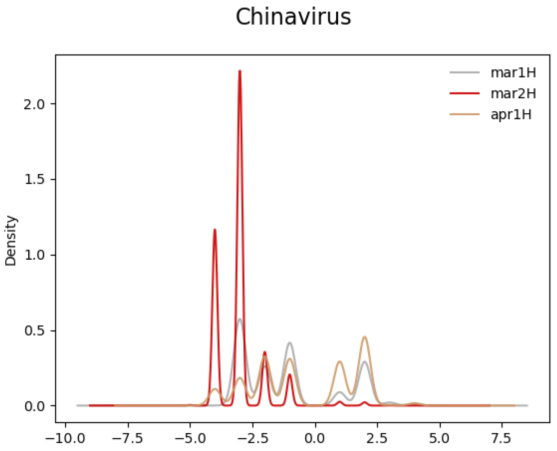
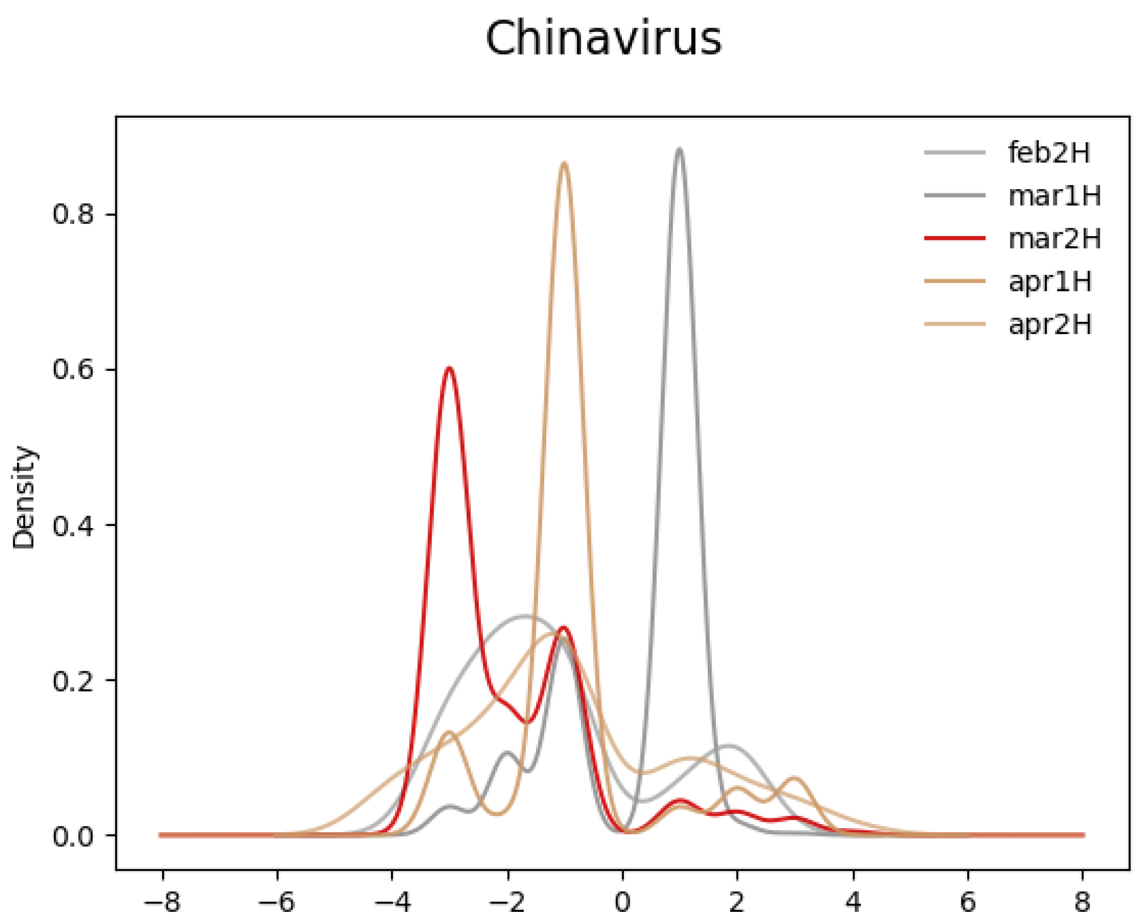
  • A novel empirical analysis of the semantics of the term “Chinavirus”:
    (a)
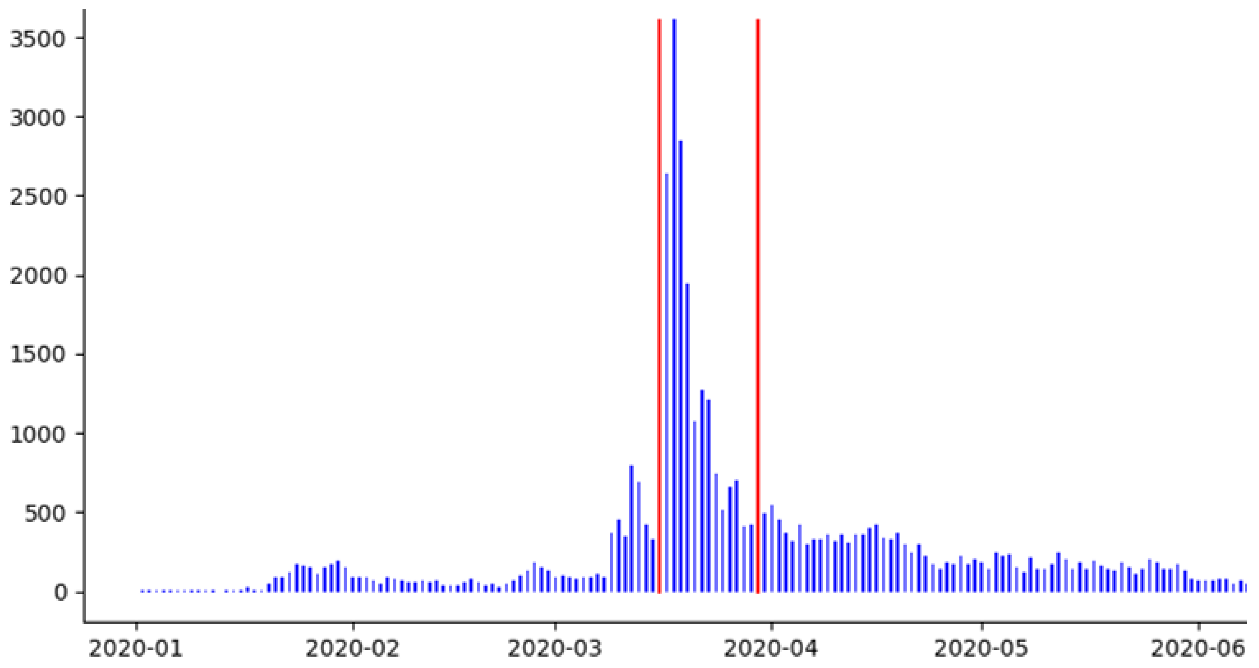
    Along the time dimension, the term took on significantly, albeit temporarily, more negative sentiment soon after its use by the White House in March 2020;
    (b)
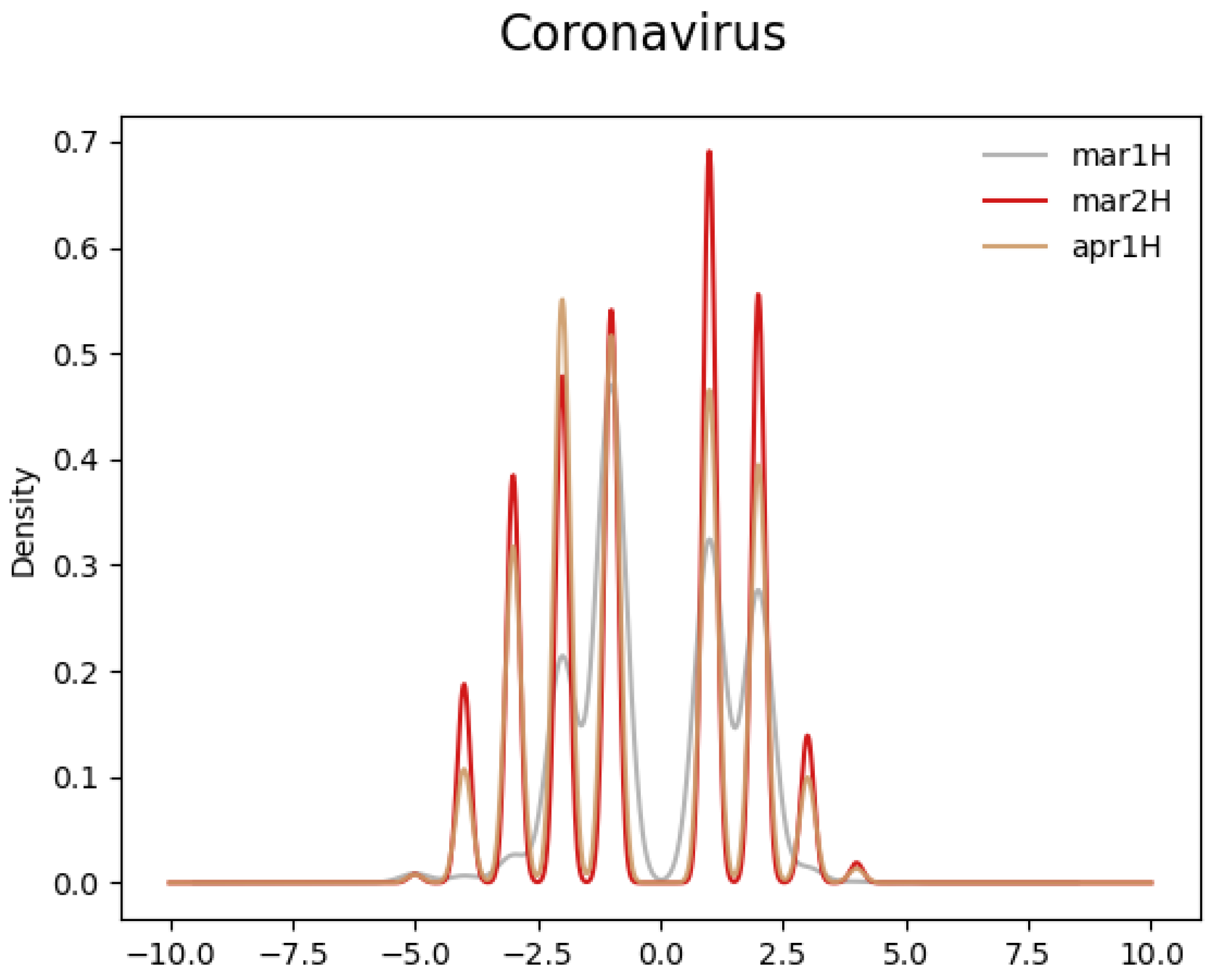
    Compared to the control term “Coronavirus”, the semantics of “Chinavirus” diverged significantly in March 2020.

2. Materials and Methods

2.1. Notation and Terminology

We use [ N ] to denote the set of natural numbers { 1 , 2 , , N } . For any nonnegative functions f ( · ) and g ( · ) on the set of natural numbers, we write
f ( n ) O ( g ( n ) ) if lim sup n f ( n ) g ( n ) < o ( g ( n ) ) if lim sup n f ( n ) g ( n ) = 0
For any given set S of words and phrases (collectively referred to as “terms” hereinafter), S c refers to the complement of S in some corpus. We denote a single-layer and undirected graph by G : = ( V , E ) having | V | = : N terms (nodes) denoted { 1 , 2 , , N } and | E | = : m edges. A denotes the unweighted adjacency matrix of G , so the rows and columns of A are indexed by the set of terms [ N ] and A i j equals 1 (respectively, 0) if there is an (respectively, no) edge between the nodes i and j, or in other words, the terms i and j appeared in a tweet together. For two subsets of nodes S a , S b [ N ] , the total number of edges between the nodes in S a and those in S b is denoted by e ( S a , S b ) . Given k 1 and a pair of terms i and j, let w i j , k be the reciprocal (respectively, 0) of the number of intervening terms between i and j in the k-th tweet if i and j were (respectively, not) present in the k-th tweet. Let w i j : = k [ | C | ] w i j , k , where | C | denotes the size of the corpus in terms of the number of tweets. Let W denote the N × N weighted matrix whose ( i , j ) -th element is w i j [ j [ N ] w i j ] 1 , which is the row-normalized transform of w i j . Then, the weighted adjacency matrix A is defined by the elementwise product of A and W , i.e., A i j : = A i j W i j for all i , j [ N ] . A is the main matrix that we work with in this paper. The weighted matrix is created with the notion that the closer the terms are in a text, the stronger their semantic relationship. The degree of node i [ N ] is the sum of the i-th row of A and is denoted by d ( v i ) or, simply, d i .
For a subset of nodes S V , its volume v o l ( S ) is defined to be the sum of the degrees of all the nodes in S , i.e., v o l ( S ) : = i S d i . We denote the number of outgoing edges from a set of nodes S by ( S ) : = | { ( i , j ) : A i j > 0 , i S , j S c } | . The conductance ϕ ( S ) of a set of nodes S V is defined as ϕ ( S ) : = ( S ) / v o l ( S ) . The conductance ϕ ( G ) of a graph G denotes the minimum among all ϕ ( S ) where S V satisfies v o l ( S ) v o l ( V ) / 2 . Clearly, ϕ ( V ) = 0 . The two-sided vertex boundary δ ( S ) of a set of nodes S is defined as δ ( S ) : = { v : v S and e ( v , S c ) > 0 } { v : v S c and e ( v , S ) > 0 } .
Following [52], we define the cost of a finite path ( S 0 , S 1 , , S t ) associated with the set process ( S t , t 0 ) to be
cos t ( S 0 , S 1 , , S t ) : = v o l ( S 0 ) + i = 1 t v o l ( S i Δ S i 1 + ( S i 1 ) ) ,
where Δ denotes the symmetric difference of sets.
For a given target term v 0 , the contextual words for v 0 are those that are more strongly associated with v 0 than any other target word, where the strength of this association is measured by the edge weights. The contextual words for v 0 are identified by its local cluster, which we discuss next.

2.2. Local Graph Clustering Algorithm in [52]

Our approach adapts a general-purpose local clustering algorithm from the applied probability theory literature [52]. It is a variation of the evolving set process (ESP), where a set evolves depending on the transition probability to other sets defined by their constituent vertices. In summary, the algorithm simulates a Markov chain (called Vb-ESP) on a subset of nodes of a graph until a specific stopping time that is defined in terms of target conductance, set volume, and cost is reached. The end result is a nonexpanding set of a fixed, user-specified volume that constitutes the dimension of the target term embedding. For a detailed treatment of the technique and the technical details of its development, we refer to reference [52]. For the sake of clarity, we restate the local clustering algorithm as proposed in [52] as Algorithms 1 and 2. In Section 2.3, we describe how we adapt Algorithms 1 and 2 to semantic term embedding and change detection tasks.

2.3. Adapting the Local Graph Clustering Algorithm for Semantic Analysis

A necessary step to precede Algorithms 1 and 2 is the construction of a “term-by-term” matrix to which the algorithms are applied. The entries in the matrix correspond to the Hamming distance between a given pair of terms. Details of the preprocessing step are given in Section 3. The inputs into Algorithm 1 are integers T (the maximum number of algorithm iterations), B (total budget for costs incurred in terms of incremental changes made in obtaining S ), κ (the threshold volume of S ), and Φ (target conductance). S t ( v 0 ) denotes the subset of V that contains the target term v 0 at time t. When the target term is obvious in the context or is irrelevant, S t is used. The finite sequence ( S t , t [ T ] ) denotes a stochastically evolving set process (ESP) and ( v t , t [ T ] ) denotes a Markov chain over the nodes of V . The desired cluster of contextual terms S for the target term v 0 results from an ESP { S t } by adding and removing terms chosen via a lazy Markov chain { v t } on V.
Next, we describe the adaptation of Algorithm 1 to the task of semantic analysis.
Line 1: S is initially set to S 0 : = { v 0 } . For the purposes of our empirical demonstration, v 0 here is set to either of { C h i n a v i r u s , C o r o n a v i r u s } and their equivalent terms as shown in Table 1.
Lines 2–4: Given { v t 1 = u } at step t 1 , we sample (in Lines 3 and 4) v t at step t based on the probability kernel p ( u , · ) , where the transition probability kernel p ( · , · ) for the Markov chain v t is given by
p ( u , w ) : = P ( v t = w | v t 1 = u ) = 1 / [ 2 d ( u ) ] if   ( u , w ) E 1 / 2 if   u = w 0 otherwise
Define p ( u , A ) : = w A p ( u , w ) for A V . Line 5: Having chosen v t at step t, we sample a threshold Z uniformly between 0 and p ( v t , S t 1 ) , where S t 1 is the value of the ESP at step t 1 .
Algorithm 1 GenerateSamples [52]
     Input: Target term v 0 , nonzero integers T , B , κ , target conductance Φ [ 0 , 1 ] .
     Output: A set S τ from the volume-biased ESP with the stopping time τ depending on input parameters τ = τ ( T , B , Φ , κ ) .
     Internal State: A set S τ from the volume-biased ESP with τ = τ ( T , B , Φ , κ ) ; the current location v t of the random walk; ( S t ) , v o l ( S t ) , and c o s t ( S 0 , , S t ) for the current set S t .
1:
Initialize S = S 0 = { v 0 }
2:
for t = 1 to T do
3:
    Given v t 1 , select v t with probability
4:
        p ( v t 1 , v t ) and update X v t
5:
    Lookup p ( v t , S t 1 ) and pick Z U n i f [ 0 , p ( v t , S t 1 ) ] .
6:
    Define S t = { u | p ( u , S t 1 ) Z } , D = .
7:
    for all  u δ ( S t 1 )  do
8:
        if  p ( u , S t 1 ) Z and u S t 1 Δ S t  then
9:
           Add u to D
10:
        end if
11:
    end for
12:
    Update v o l ( S t ) and cost( S 0 , , S t )
13:
    if  t = T or cost ( S 0 , , S t ) > B  then
14:
        return  S = S t 1 Δ D
15:
    end if
16:
    Update S S t = S t 1 Δ D by adding or removing vertices in D from S
17:
    Update ( S t ) , ϕ ( S t ) = ( S t ) / v o l ( S t )
18:
    if  ϕ ( S t ) Φ and v o l ( S t ) κ  then
19:
        return  S
20:
    end if
21:
end for
Algorithm 2 EvoPar( v , k , ϕ , ϵ ) [52]
Input: Target term v 0 , target volume k, target conductance ϕ [ 0 , 1 ] , a constant ϵ ( 0 , 1 ) .
Output: A set S of vertices.
1:
T ϵ log k / 6 ϕ
2:
Run in parallel k ϵ / 2 independent copies of GenerateSample( v 0 , T , , κ ϵ / 2 ( k ) , Φ ϵ / 2 ( ϕ ) )
3:
if Any of the copies finds S satisfying v o l ( S ) κ ϵ / 2 ( k ) and ϕ ( S ) Φ ϵ / 2 ( ϕ ) then
4:
    return  S
5:
end if
Line 6: S t is obtained at step t from S t 1 using the threshold Z and the kernel p ( · , · ) . The threshold Z is needed to ensure that { S t } defined in Line 6 does not vanish. This is because { S t } can vanish if the threshold probability Z, which is used in adding nodes, can be arbitrarily high. This variant of ESP is coupled with the random walk { v t } and is called Vb-ESP. The set transition probability kernel K ( · , · ) , where K ( A , B ) : = P ( S t = B | S t 1 = A ) , is adjusted by the product of the ratio of the volumes of the two arguments of K ( · , · ) . It is well known that the mixing time of the underlying Markov chain { v t } in Vb-ESP is bounded by the Cheeger expansion constant. With constant probability, this process results in set S with conductance and volume close (to be more precise, ϕ ( S ) = O ( ϕ / ϵ ) for target conductance ϕ and parameter ϵ ( 0 , 1 ) , and vol ( S ) = O ( k 1 + ϵ ) for target volume k) to the desired quantities in O ( log N ) time complexity. We set the target conductance to 0.3 and the volume threshold to 0.01 N . Multiple iterations of it are run to ensure the resulting S meets the specific thresholds for conductance and volume.
Lines 7–11: For a set S , p ( u , S ) denotes the transition probability from the current term u to any w S :
p ( u , S ) : = w S p ( u , w ) = 1 2 e ( u , S ) d ( u ) + 1 { u S }
where e ( u , S ) : = | { ( u , w ) : ( u , w ) E , u S } | . The stationary probability distribution for the nodes in the graph is given by
π S ( u ) = d ( u ) / v o l ( S ) if   u S 0 otherwise
The transition probability matrix for the random walk described here is expressed as P : = 1 2 ( M 1 A + I ) , where M is the diagonal matrix whose element M i i is the sum of the i-th row of A , i.e., degree of the i-th node in A .
Line 12: We update the values for v o l ( S t ) and cost ( S 0 , , S t ) , which are tested against the stopping conditions in Lines 13 and 18. Line 13: A stopping condition based on the number of iterations T and total cost B for the value in Line 12. Line 17: We update the values for the number of outgoing edges from S t and the conductance to test against the stopping conditions in Line 18. Line 18: A stopping condition based on conductance Φ and volume κ for the value in Line 17.
Given current S 1 , the ESP proceeds to the next state S 2 in Algorithm 2. Given the threshold Z Unif [ 0 , 1 ] and S 2 = { u : p ( u , S 1 ) Z ) , the volume-based ESP is an ESP with the transition kernel:
K ^ ( S , S ) = v o l ( S ) v o l ( S ) K ( S , S )
where K ( S , S ) is the transition kernel for the ESP. Due to the Diaconis–Fill coupling, the transition probability from the current state ( v t , S t ) is
P [ v t + 1 = w : v t = u , S t = S ] = p ( u , w ) P [ S t + 1 = S : S t = S , v t + 1 = w ] = K ( S , S ) 1 { w S } P [ w S t + 1 : S t = S ]
Hence, a node v t + 1 is selected from the transition kernel, and S t + 1 from the ESP transition kernel, from those sets containing v t + 1 .
Below, we describe the adaptation of Algorithm 2 for the purpose of semantic analysis.
Input: The inputs into Algorithm 2 are a starting vertex v V , a target conductance ϕ ( 0 , 1 ) , target volume k > 0 , and ϵ ( 0 , 1 ) .
Line 1: Set the maximum total number of iterations T as given.
Line 2: Run in parallel withAlgorithm 1 with the given set of parameters. Multiple threads of local clustering are run in parallel since there is a chance that a target term v 0 exits its cluster S t at some t [ T ] .
Lines 3 and 4: When the stopping time τ is reached by the algorithm, the S τ that is returned is the contextual set S for the target term v 0 . With inputs k (target volume), Φ (target conductance), and constant ϵ ( 0 , 1 ) into the algorithm, the contextual cluster S output by the algorithm has conductance O ( Φ / ϵ ) and volume of at least half of any set with conductance at most Φ and volume at most m 1 ϵ / c with absolute constant c > 0 .
For any stopping time τ , this procedure has been shown to output at least one incidence of S t with ϕ ( S t ) O ( log v o l ( S τ ) / τ ) [52].
We apply this algorithm to the corpus comprising tweets containing “Chinavirus”, “Coronavirus”, and similar terms, which we denote by “equivalence classes of terms” for nine 2-week periods surrounding the second half of March 2020. The significance of this time period is due to the White House’s use of the term “Chinavirus” on at least 20 occasions [53] during this period. In Table 1, we list all the target terms by equivalence classes we performed local clustering on. Once local clusters for each target term are identified, we look up term-level sentiment scores for all terms in the clusters using the package AFINN [54] in the Python programming language. It uses a numerical scale from −5 to +5, with −5 denoting the most negative, +5 the most positive terms, and 0 the neutral sentiment. We then compare the sentiment score distribution of the “Chinavirus” cluster in the second half of March to those in other 2-week periods (“temporal control”) as well as “Coronavirus” clusters over the same time periods (“cross-sectional control”).

3. Datasets

Our data are composed of geotagged public tweets containing the target query terms “Chinavirus”, “Coronavirus”, and variants thereof originating from within the United States from the period spanning the second half of January through the second half of May 2020. The tweets were limited to those written in the English language. The tweets and the accompanying metadata were downloaded from the Twitter Server via the Twitter Developer Application Programming Interface (API) Early Access version 2 between 20 April and 11 May 2021.
Several variations of “Chinavirus” and “Coronavirus” were used on Twitter in terms of spelling and concatenations with other words. In our preprocessing step, we grouped these variations together into a set that we call “equivalence class”. As a result, we had two “equivalence classes”, one for each of “Chinavirus” and “Coronavirus”, and treated each term in an equivalence class as the same, in effect making the cluster for each target term a union of clusters of the constituent terms in its equivalence class. The compositions of these equivalence classes for the two target terms are shown below in Table 1.
We used the NLTK library in Python to apply the standard preprocessing step of tokenization and normalization and removal of frequent stop words and rare contexts that appear fewer than 100 times in our Twitter corpus. We applied other common preprocessing steps to remove capitalization and apply lemmatization and stemming.
The resulting dataset consisted of a corpus of 9,275,358 words representing a vocabulary size of 119,614 terms based on 747,737 tweets posted by 204,488 authors. Table 2 displays the breakdown of the dataset by 2-week intervals.
In Section 4, we analyze the progression of the semantics of the equivalence classes of terms “Chinavirus” versus “Coronavirus”, where the latter term is used as a control. We then test the efficacy of our method with (1) the benchmark Word2Vec embeddings and (2) studies on the effect of “Chinavirus” on public sentiment as reported in the literature.

4. Results

Soon after the phrase “Chinavirus” started appearing in the administration’s public statements on 16 March 2020, the number of tweets containing the phrase “Chinavirus” sharply increased. As is evident in Figure 1, the daily count of such tweets increased from less than 500 to more than 3500.
To identify the clusters of the two phrases, we perform local clustering, as discussed in Section 2.3, and its algorithm, presented in Section 2 as the Algorithms 1 and 2. We assigned the equivalence classes of “Chinavirus” and “Coronavirus” to be the starting nodes v 0 , with the latter as a control node to place the temporal progression of the former in perspective. Below is the set of words that are clustered together with “Chinavirus” for the first half of March (Table 3), followed by the cluster for the second half of March (Table 4). One can readily see that the sentiment noticeably became negative in the second half.
As a reference, the clusters for the control term “Coronavirus” for the same two periods are shown in Table 5 and Table 6. Compared to the clusters for “Chinavirus” over the same periods, one can see that there is no noticeable variation in sentiment.
We now look at the distributions of the sentiment scores for both terms over time. Figure 2 displays the temporal progression of the distribution of the contextual words by their sentiment scores for “Chinavirus”, where more negative scores denote relatively more negative words and positive scores positive on the scale of −5 to 5. It is apparent that the distribution is more concentrated around a negative score of −3 on 2 March, when the White House made use of the phrase “Chinavirus”. More formally, using the Kolmogorov–Smirnov test as implemented in the SciPy Python package, we are able to reject, with a p-value of less than 0.001, the null hypothesis that the sentiment scores on 2 March came from the same distribution as those in the other 2-week periods. Using the Mann–Whitney U-test in the SciPy package, we conclude, with a p-value of less than 0.001, in favor of the hypothesis that the sentiment scores on 2 March are lower than those in the other periods and the sentiment scores of the cross-sectional control, “Coronavirus” (see Section 2 for discussion).
As a point of reference, Figure 3 displays a similar chart for the term “Coronavirus”. Compared to “Chinavirus”, there is no visible shift in the distribution of the sentiment scores.
Next, we checked the effectiveness of our method in two ways. First, we note that this shift in the sentiment distribution of “Chinavirus” in March, compared to its distributions in previous periods and those of “Coronavirus”, is consistent with what was reported in references [48,49,50]. Second, we transformed the vocabulary in each 2-week period into Word2Vec representations using the Gensim package in the Python programming language and identified a set of synonyms for each of the two target terms. Synonyms in Word2Vec are defined in terms of cosine similarity, and we classified terms in the vocabulary as synonyms if their cosine similarity measures were at least 0.3. Figure 2 and Figure 4 show that the sentiment of the synonyms of “Chinavirus” clearly shifted more negative compared to surrounding periods in the second half of March 2020.

5. Discussion

As new additions to the English language, terms such as “Chinavirus” present a significant challenge when one tries to ascertain its semantics and perform analogy tasks to other related terms such as “Coronavirus”. In the absence of a definitive source for the semantics of such terms, we propose to characterize the semantics of novel terms by looking at their clusters of strongly associated words and phrases, staying true to John R. Firth’s famous quote that “[y]ou shall know a word by the company it keeps” [55]. To obtainthe granular clustering that allows for a differentiation of two closely related terms, we use “local” clustering, as implemented in [52], to build out an informative cluster of contextual words, starting with the singleton set containing the target term and stopping once a target conductance or cluster size is reached. By comparing the composition of the term’s clusters’ composition over time and the “control” terms, one can reasonably infer if the term’s semantics have changed over time and how it compares to other terms.
Our approach makes the following contributions. Compared to existing graph clustering algorithms, our method identifies a local cluster of contextual words that is tailored only to a specific target term, thus making the cluster more informative and compact for inferring term-level semantics. Because our approach does not make use of the information about global structures of corpus graphs, it avoids performing unnecessary work, such as clustering all words in the input data, and hence is computationally efficient with constant time complexity. Our method allows clusters of two different target terms to overlap, which is more intuitive and consistent with how one thinks about the semantics of words than partitioning contextual words into disjoint clusters, as performed in global clustering and some of the subspace segmentation methods. Lastly, we provide a rigorous confirmation of the results in the existing literature that observe that the use of “Chinavirus” and its close variants by the White House in March of 2020 is associated with a significant increase in negative sentiment in public discourse compared to earlier months and compared to “Coronavirus” as the control.
For future study, one possible application of local clustering is the construction of a thesaurus. The current approach to thesaurus construction does not allow for efficient and intuitive detection of the so-called “change-points” in a word’s meaning in time. Manually constructing thesauri at various points in time and comparing the composition of the sets of synonyms is belaboring at best and lacks rigor. Applying local clustering, one could infer from any statistically significant change in cluster composition, from one period to another, a change-point in the thesaurus, suggesting that semantic changes in certain words took place.

Author Contributions

Conceptualization: N.H.; methodology, N.H., S.B. and S.C.; software: N.H.; validation: N.H.; formal analysis: N.H. and S.C.; investigation: N.H., Y.D., S.B. and S.C.; resources: N.H., Y.D., S.B. and S.C.; data curation: N.H.; writing—original draft preparation: N.H.; writing—review and editing: Y.D., S.B., S.C. and N.H.; visualization: N.H.; supervision: Y.D., S.B. and S.C.; project administration: Y.D., S.B. and S.C. All authors have read and agreed to the published version of the manuscript.

Funding

S. Chatterjee was partially supported by the NSF DMS grant 2154564 and PSC-CUNY Enhanced Research Award 64673-00 52.

Data Availability Statement

The data presented in this study are openly available in the https://developer.twitter.com (Twitter Developer API), accessed on 8 May 2021. The data presented in this study are available on request from the corresponding author. The data are not publicly available due to the large size of the files.

Conflicts of Interest

The authors declare no conflict of interest.

References

  1. Liebeskind, C.; Dagan, I.; Schler, J. Statistical thesaurus construction for a morphologically rich language. In Proceedings of the Sixth International Workshop on Semantic Evaluation, Montréal, QC, Canada, 7–8 June 2012; pp. 59–64. [Google Scholar]
  2. Zaragoza, M.Q.; Torres, L.S.; Basdevant, J. Translating Knowledge Representations with Monolingual Word Embeddings: The Case of a Thesaurus on Corporate Non-Financial Reporting. In Proceedings of the 6th International Workshop on Computational Terminology, Marseille, France, 11–16 May 2020. [Google Scholar]
  3. Loukachevitch, N.; Parkhomenko, E. Thesaurus Verification Based on Distributional Similarities. In Proceedings of the 10th Global Wordnet Conference, Wroclaw, Poland, 23–27 July 2019; pp. 16–23. [Google Scholar]
  4. Levy, O.; Goldberg, Y.; Dagan, I. Improving distributional similarity with lessons learned from word embeddings. Trans. Assoc. Comput. Linguist. 2015, 3, 211–225. [Google Scholar] [CrossRef]
  5. Baroni, M.; Dinu, G.; Kruszewski, G. Don’t count, predict! a systematic comparison of context-counting vs. context-predicting semantic vectors. In Proceedings of the 52nd Annual Meeting of the Association for Computational Linguistics (Volume 1: Long Papers), Baltimore, MD, USA, 22–27 June 2014; pp. 238–247. [Google Scholar]
  6. Pennington, J.; Socher, R.; Manning, C.D. Glove: Global vectors for word representation. In Proceedings of the 2014 Conference on Empirical Methods in Natural Language Processing (EMNLP), Doha, Qatar, 25–29 October 2014; pp. 1532–1543. [Google Scholar]
  7. Eckart, C.; Young, G. The approximation of one matrix by another of lower rank. Psychometrika 1936, 1, 211–218. [Google Scholar] [CrossRef]
  8. Schütze, H. Automatic word sense discrimination. Comput. Linguist. 1998, 24, 97–123. [Google Scholar]
  9. Horn, R.A.; Johnson, C.R. Matrix Analysis; Cambridge University Press: Cambridge, UK, 2012. [Google Scholar]
  10. Deerwester, S.; Dumais, S.T.; Furnas, G.W.; Landauer, T.K.; Harshman, R. Indexing by latent semantic analysis. JASIST 1990, 41, 391–407. [Google Scholar] [CrossRef]
  11. McDonald, S. Environmental Determinants of Lexical Processing Effort. Doctoral Dissertation, University of Edinburgh, Edinburgh, UK, 2000. [Google Scholar]
  12. Lemaire, B.; Denhière, G. Incremental construction of an associative network from a corpus. In Proceedings of the Annual Meeting of the Cognitive Science Society, Chicago, IL, USA, 4–7 August 2004; Volume 26. [Google Scholar]
  13. Bordenave, C.; Lelarge, M.; Massoulié, L. Non-backtracking spectrum of random graphs: Community detection and non-regular ramanujan graphs. In Proceedings of the 2015 IEEE 56th Annual Symposium on Foundations of Computer Science, Berkeley, CA, USA, 2 February 2015; pp. 1347–1357. [Google Scholar]
  14. Saade, A.; Krzakala, F.; Zdeborová, L. Spectral clustering of graphs with the bethe hessian. arXiv 2014, arXiv:1406.1880. [Google Scholar]
  15. Dall’Amico, L.; Couillet, R.; Tremblay, N. Revisiting the bethe-hessian: Improved community detection in sparse heterogeneous graphs. arXiv 2019, arXiv:1901.09715. [Google Scholar]
  16. Le, C.M.; Levina, E. Estimating the number of communities in networks by spectral methods. arXiv 2015, arXiv:1507.00827. [Google Scholar]
  17. Coste, S.; Zhu, Y. Eigenvalues of the non-backtracking operator detached from the bulk. Random Matrices Theory Appl. 2021, 10, 215002. [Google Scholar] [CrossRef]
  18. Dall’Amico, L.; Couillet, R.; Tremblay, N. Community detection in sparse time-evolving graphs with a dynamical bethe-hessian. arXiv 2020, arXiv:2006.04510. [Google Scholar]
  19. Dumais, S.T. Latent semantic analysis. Annu. Rev. Inf. Sci. Technol. 2004, 38, 188–230. [Google Scholar] [CrossRef]
  20. Lund, K.; Burgess, C. Hyperspace analogue to language (hal): A general model semantic representation. In Brain and Cognition; Academic Press Inc Jnl-Comp Subscriptions: San Diego, CA, USA, 1996; Volume 30, pp. 92101–94495. [Google Scholar]
  21. Rohde, D.; Gonnerman, L.M.; Plaut, D.C. An improved model of semantic similarity based on lexical co-occurrence. Commun. ACM 2006, 8, 116. [Google Scholar]
  22. Bullinaria, J.A.; Levy, J.P. Extracting semantic representations from word co-occurrence statistics: A computational study. Behav. Res. Methods 2007, 39, 510–526. [Google Scholar] [CrossRef] [PubMed] [Green Version]
  23. Collobert, R. Word embeddings through hellinger pca. In Proceedings of the 14th Conference of the European Chapter of the Association for Computational Linguistics, Gothenburg, Sweden, 26–30 April 2014. [Google Scholar]
  24. Hamerly, G.; Charles, E. Learning the k in k-means. Adv. Neural Inf. Process. Syst. 2003, 16, 281–288. [Google Scholar]
  25. Har-Peled, S.; Soham, M. On coresets for k-means and k-median clustering. In Proceedings of the Thirty-Sixth Annual ACM Symposium on Theory of Computing, Chicago, IL, USA, 13–15 June 2004. [Google Scholar]
  26. Biemann, C. Chinese whispers-an efficient graph clustering algorithm and its application to natural language processing problems. In Proceedings of the TextGraphs: The First Workshop on Graph Based Methods for Natural Language Processing, New York, NY, USA, 9 June 2006. [Google Scholar]
  27. Cai, Y.; Zhang, Z.; Cai, Z.; Liu, X.; Jiang, X. Hypergraph-structured autoencoder for unsupervised and semisupervised classification of hyperspectral image. IEEE Geosci. Remote Sens. Lett. 2021, 19, 5503505. [Google Scholar] [CrossRef]
  28. Lei, J.; Li, X.; Peng, B.; Fang, L.; Ling, N.; Huang, Q. Deep spatial–spectral subspace clustering for hyperspectral image. IEEE Trans. Circuits Syst. Video Technol. 2021, 31, 2686–2697. [Google Scholar] [CrossRef]
  29. Sun, J.; Wang, W.; Wei, X.; Fang, L.; Tang, X.; Xu, Y.; Yu, H.; Yao, W. Deep clustering with intraclass distance constraint for hyperspectral images. IEEE Trans. Geosci. Remote Sens. 2021, 59, 4135–4149. [Google Scholar] [CrossRef]
  30. PBickel, J.; Sarkar, P. Hypothesis testing for automated community detection in networks. J. R. Stat. Soc. Ser. B Stat. Methodol. 2016, 78, 253–273. [Google Scholar] [CrossRef]
  31. Chen, K.; Lei, J. Network cross-validation for determining the number of communities in network data. J. Am. Stat. Assoc. 2018, 113, 241–251. [Google Scholar] [CrossRef] [Green Version]
  32. Li, T.; Levina, E.; Zhu, J. Network cross-validation by edge sampling. Biometrika 2020, 107, 257–276. [Google Scholar] [CrossRef]
  33. Yan, B.; Sarkar, P.; Cheng, X. Provable estimation of the number of blocks in block models. In Proceedings of the International Conference on Artificial Intelligence and Statistics, Playa Blanca, Lanzarote, Canary Islands, 9–11 April 2018; pp. 1185–1194. [Google Scholar]
  34. Hu, J.; Qin, H.; Yan, T.; Zhao, Y. Corrected bayesian information criterion for stochastic block models. J. Am. Stat. Assoc. 2020, 115, 1771–1783. [Google Scholar] [CrossRef]
  35. Ma, S.; Su, L.; Zhang, Y. Determining the number of communities in degree-corrected stochastic block models. Mach Learn Res. 2021, 22, 1–63. [Google Scholar]
  36. Axel-Cyrille, N.N. SIGNUM: A graph algorithm for terminology extraction. In Proceedings of the International Conference on Intelligent Text Processing and Computational Linguistics, Haifa, Israel, 17–23 February 2008; Springer: Berlin/Heidelberg, Germany, 2008. [Google Scholar]
  37. Mihalcea, R.; Tarau, P. Textrank: Bringing order into text. In Proceedings of the 2004 Conference on Empirical Methods in Natural Language Processing, Barcelona, Spain, 25–26 July 2004. [Google Scholar]
  38. Ngomo, N.; Axel-Cyrille;Schumacher, F. Borderflow: A local graph clustering algorithm for natural language processing. In International Conference on Intelligent Text Processing and Computational Linguistics; Springer: Berlin/Heidelberg, Germany, 2009. [Google Scholar]
  39. Li, K.; Qin, Y.; Ling, Q.; Wang, Y.; Lin, Z.; An, W. Self-supervised deep subspace clustering for hyperspectral images with adaptive selfexpressive coefficient matrix initialization. IEEE J. Sel. Topics Appl. Earth Observ. Remote Sens. 2021, 14, 3215–3227. [Google Scholar] [CrossRef]
  40. Eismann, M.T.; Stocker, A.D.; Nasrabadi, N.M. Automated hyperspectral cueing for civilian search and rescue. Proc. IEEE 2009, 97, 1031–1055. [Google Scholar] [CrossRef]
  41. Ester, M.; Kriegel, H.-P.; Sander, J.; Xu, X. A density-based algorithm for discovering clusters in large spatial databases with noise. Proc. KDD 1996, 96, 226–231. [Google Scholar]
  42. Zhang, H.; Kang, J.; Xu, X.; Zhang, L. Accessing the temporal and spectral features in crop type mapping using multi-temporal sentinel-2 imagery: A case study of Yi’an County, Heilongjiang province, China. Comput. Electron. Agric. 2020, 176, 105618. [Google Scholar] [CrossRef]
  43. Lloyd, S. Least squares quantization in PCM. IEEE Trans. Inf. Theory 1982, 28, 129–137. [Google Scholar] [CrossRef] [Green Version]
  44. Bezdek, J.C. Pattern Recognition with Fuzzy Objective Function Algorithms; Springer: Berlin, Germany, 2013. [Google Scholar]
  45. Elhamifar, E.; René, V. Sparse subspace clustering: Algorithm, theory, and applications. IEEE Trans. Pattern Anal. Mach. Intell. 2013, 35, 2765–2781. [Google Scholar] [CrossRef] [PubMed] [Green Version]
  46. Huang, S.; Zhang, H.; Pižurica, A. Subspace clustering for hyperspectral images via dictionary learning with adaptive regularization. IEEE Trans. Geosci. Remote Sens. 2021, 60, 5524017. [Google Scholar] [CrossRef]
  47. Liu, G.; Lin, Z.; Yan, S.; Sun, J.; Yu, Y.; Ma, Y. Robust recovery of subspace structures by low-rank representation. IEEE Trans. Pattern Anal. Mach. Intell. 2012, 35, 171–184. [Google Scholar] [CrossRef]
  48. Reny, T.; Barreto, M. Xenophobia in the time of pandemic: Othering, anti-Asian attitudes, and COVID-19. Politics Groups Identities 2020, 10, 209–232. [Google Scholar] [CrossRef]
  49. Tsai, J.Y.; Phua, J.; Pan, S.; Yang, C. Intergroup contact, COVID-19 news consumption, and the moderating role of digital media trust on prejudice toward Asians in the United States: Cross-sectional study. J. Med. Internet Res. 2020, 22, e22767. [Google Scholar] [CrossRef] [PubMed]
  50. Hswen, Y.; Xu, X.; Hing, A.; Hawkins, J.B.; Brownstein, J.S.; Gee, G.C. Association of ’# Covid19’ Versus ’# Chinesevirus’ with Anti-Asian Sentiments on Twitter: March 9–23, 2020. Am. J. Public Health 2021, 111, 956–964. [Google Scholar] [PubMed]
  51. Mossel, E.; Neeman, J.; Sly, A. A proof of the block model threshold conjecture. Combinatorica 2018, 38, 665–708. [Google Scholar] [CrossRef] [Green Version]
  52. Andersen, R.; Gharan, S.; Peres, Y.; Trevisan, L. Almost optimal local graph clustering using evolving sets. J. ACM 2016, 63, 1–31. [Google Scholar] [CrossRef]
  53. “Donald Trump’s ‘Chinese Virus’: The Politics of Naming”, The Conversation. Available online: https://theconversation.com/donald-trumps-chinese-virus-the-politics-of-naming-136796 (accessed on 21 October 2021).
  54. Nielsen, F. A new ANEW: Evaluation of a word list for sentiment analysis in microblogs. In Proceedings of the ESWC 2011 Workshop on ’Making Sense of Microposts’: Big Things Come in Small Packages, Heraklion, Crete, 30 May 2011; pp. 93–98. [Google Scholar]
  55. Firth, J. A synopsis of linguistic theory, 1930–1955. In Studies in Linguistic Analysis; Blackwell: Oxford, UK, 1957. [Google Scholar]
Figure 1. Daily count of tweets containing “Chinavirus”. The red vertical lines denote the period March 16 March through 31 March 2020 when the phrase “Chinavirus” and its variants were used by the White House.
Make 05 00008 g001
Figure 2. Sentiment score distribution of contextual words of “Chinavirus”.
Make 05 00008 g002
Figure 3. Sentiment score distribution of contextual words of “Coronavirus”.
Make 05 00008 g003
Figure 4. Sentiment score distribution of Word2Vec terms with cosine similarity score of at least 0.3 compared to “Chinavirus”.
Make 05 00008 g004
Table 1. Equivalence classes of target terms.
“Chinavirus”“Coronavirus”
ChinavirusChinacovidCoronavirusCoronaviruses
ChinavirusesChinesecovidCovidvirusCovidviruses
ChinesevirusesChinesevirusCaronavirusCaronaviruses
ChinacoronaWuhanvirusesVirus-coronaVirus-covid
WuhancovidWuhancoronaCoronafluCoronoviruses
CCPVirusCCPCoronavirusCoronacovidCovidcorona
WuhanchinavirusCoronaoutbreakCoronovirus
Wuhanchinaviruses
Chinawuhanvirus
Chinesecoronavirus
Chinesecoronaviruses
ChineseCommunistPartyvirus
ChineseCommunistPartyviruses
Table 2. Descriptions of corpora by 2-week intervals.
Period aWords bVocabulary bTweets bAuthorIDs b
Jan2H123,87410,98510,4628881
Feb1H129,54512,28610,7487190
Feb2H363,39420,11317,63910,927
Mar1H2,261,05952,724176,38693,339
Mar2H2,745,58965,138215,90899,069
Apr1H1,322,02545,44499,87447,457
Apr2H866,07437,13765,13931,404
May1H593,13430,62143,70621,972
May2H432,83225,62032,42517,494
a “1H” represents the first half and “2H” the second half; b represents the numbers of unique counts for each 2-week interval.
Table 3. Cluster of “Chinavirus”, 1–15 March 2020.
restaurantlivestockdivulgehotpotwheelfloor
remainderinitiativeChinesegaslitstormfight
designationsacrificemarriedundonefunnyfront
inevitablehistoricalforwardglobalsadlyarmy
sabotagingpossiblequickerinsultguesssight
investmenttogetherstrategyfasterslumpdrug
supervisoringenioussuspendspiralunitealive
Table 4. Cluster of “Chinavirus”, 16–31 March 2020.
overreachquarantinecroniesapologizesexilescare
moralitypanickedkissingmoronovirusabjectstud
mournersacrificelaughtsaccusationgoofydog
antiviralbaselesslyurinecompassionpokedhoax
pollutionespionagefuckedoverwhelmedcloutloser
assassindrippingevilsprohibitionriskingalien
exposureinabilityoutrageunbecomingstrokesecrets
derailedenflamesdestroydenouncenamastenutjob
tearfuldumbkirkdebunkdischargescookingchased
buttheadrobbingselfishdangerousdiarrheacheat
debunkdespairhuaweiheartattackillprotest
screamgorillasthriveconcussionmysteryalarmed
repellantdistancechaoticmaraudingfolliesbedbug
migraineprosecutepurifierexterminateillicitracism
explodespangolinlizardreelectionfuckkloots
Table 5. Cluster of “Coronavirus”, 1–15 March 2020.
cancellationrobitussininterferegreenlitbravelynuk
disruptionshumiliatesovercomeprophecydisobeyease
animalisticequanimitypharmacyhosepipeunmasksigh
moisturizedheatstrokedecouplecheapgasservicefiery
envelopmentpropagateguillotineconfrontdirtygosh
untouchableretractioncrackheadhelplesspumpedgoofy
overeactingperpectiveconcernedfuneralpunitivepiss
perpetuatesinadequatescrambleecstaticmidgetcost
breathmintsplanetizendeadliercolonialfaceassfuel
precipitateunfriendedpopulismeducate
Table 6. Cluster of “Coronavirus”, 16–31 March 2020.
hospitablecollapsedcrackpotpumpedstrangernuk
celebrationblockheadfecklesspissingbreachease
overshadowpossessiveregardedsodexonutcasebane
excellenceexpensiverampagestabbedrecklessdirty
deprivationdisappearbunglingunstableghettorevive
panoramicapologizeevacuatecringedfuckinggoof
fucknugettesstrangledpunitivesqueakcleanlyruined
martyrdomvirulencepreventflaggingmidgetdirt
determinedreputablekickbackbadassfaceasssigh
contenderdownsidedelusionalbabble
Disclaimer/Publisher’s Note: The statements, opinions and data contained in all publications are solely those of the individual author(s) and contributor(s) and not of MDPI and/or the editor(s). MDPI and/or the editor(s) disclaim responsibility for any injury to people or property resulting from any ideas, methods, instructions or products referred to in the content.

