InvMap and Witness Simplicial Variational Auto-Encoders

Abstract

Variational auto-encoders (VAEs) are deep generative models used for unsupervised learning, however their standard version is not topology-aware in practice since the data topology may not be taken into consideration. In this paper, we propose two different approaches with the aim to preserve the topological structure between the input space and the latent representation of a VAE. Firstly, we introduce InvMap-VAE as a way to turn any dimensionality reduction technique, given an embedding it produces, into a generative model within a VAE framework providing an inverse mapping into original space. Secondly, we propose the Witness Simplicial VAE as an extension of the simplicial auto-encoder to the variational setup using a witness complex for computing the simplicial regularization, and we motivate this method theoretically using tools from algebraic topology. The Witness Simplicial VAE is independent of any dimensionality reduction technique and together with its extension, Isolandmarks Witness Simplicial VAE, preserves the persistent Betti numbers of a dataset better than a standard VAE.

1. Introduction

Topological data analysis (TDA) is a recent field in data science aiming to study the “shape” of data, or, in other words, to understand, analyse, and exploit the geometric and topological structure of data, in order to obtain relevant information. For that purpose, it combines mathematical notions essentially from algebraic topology, geometry, combinatorics, probability, and statistics, with powerful tools and algorithms studied in computational topology. Algebraic topology identifies homeomorphic objects, that is for example objects that we can deform continuously (without breaking) from one to the other, and computational topology studies the application of computation to topology by developing algorithms aiming to construct and analyse topological structures.

Nowadays, the two most famous deep generative models are the Generative Adversarial Network [1] and the variational auto-encoder (VAE) [2,3]. In this paper, we focus on the latter. The VAE, like its deterministic counter-part the auto-encoder (AE), allows to compress high dimensional input data into a lower dimensional space called the latent space, and then reconstructs the output from this compressed representation. In addition to its ability to generate new data, the VAE can, thus, be used for many applications, especially for dimensionality reduction which is useful for signal compression, high dimensional data visualisation, classification tasks, or clustering in a lower dimensional space, etc.

This paper presents in a more concise way our main work developed during Medbouhi’s master thesis [4] and provides an extension of the Witness Simplicial VAE method. We investigate here the use of TDA in order to modify the VAE with the hope that it will lead to an improvement of its performance. In particular, we try to improve its latent representation. A large part of this work is at the intersection between machine learning and TDA, this bridge is an emerging field referred to as “topological machine learning” [5]. Thus, this paper is part of the cross-talk between topologist and machine learning scientist [6]. Although the research carried out here is quite theoretical, it can potentially lead to many concrete applications in very different fields and, in particular, in robotics. For example, in a robotic context the latent space of a VAE could represent the space of configurations of a robot or the states of a system composed by a robot and its environment. In such case, an interpolation between two points in the latent space can represent a trajectory of the robot. As the input space is generally high dimensional, it might be hard to realize interpolations there. However, with a VAE one can represent the data in the latent space with less dimensions, perform interpolations in this latent space, and then generate the trajectories for motion planning. Thus, having a VAE which takes into account the data topology could help to better perform interpolations in its latent space in order to do robotics motion planning. On one side, preserving 0-homology would allow one to avoid to perform “meaningless” interpolations between two points from different connected components. On the other side, preserving 1-homology enables to keep track of possible “loops” or cyclic structures between the input and the latent space. That is why we are interested in preserving several homology orders.

The question we try to answer is: how to preserve the topology of data between the input and the latent spaces of a variational auto-encoder? Our assumption is that preserving the topology should lead to a better latent representation and this would help to perform better interpolations in the latent space. This rises many underlying questions: what exactly do we want to preserve? What kind of topological information should we keep? How do we find relevant topological information in the data? Does that depend on the problem and the data? How to preserve such topological information in a variational auto-encoder framework? Algebraic topology gives topological invariants such as the Betti numbers which are discrete whereas training a VAE implies to optimize a loss which needs to be differentiable and thus continuous. So how can we incorporate such discrete topological invariant in a continuous function?

The paper is structured as follows. Section 2 gives preliminary concepts of computational topology needed to understand some related work, our problem formulation and our method called Witness Simplicial VAE. Section 3 highlights the related work about non-linear dimensionality reduction techniques, variational auto-encoders and topology preservation. Section 4 gives implementation details for reproducibility of the experiments. Section 5 formulates the problem and shows that the standard VAE is not topology-aware in practise. Section 6 presents our first method called InvMap-VAE with its results. Section 7 does the same with our second method called Witness Simplicial VAE and its extension Isolandmarks Witness Simplicial VAE. These methods are discussed in Section 8. Finally, conclusions and future work directions are given in Section 9.

2. Notions of Computational Topology

In this section, we present briefly some notions of Computational Topology that are relevant to our work. For a complete introduction, we refer the reader to any book of computational topology, such as the one by Edelsbrunner and Harer [7], or to the theoretical background of our master thesis [4] which is self-contained. Computational topology aims to compute and develop algorithms in order to analyse topological structures, that is the shapes of considered objects. For that purpose, we introduce some notions related to simplicial complexes. The latter allow us to decompose a topological space into many simple pieces, namely the simplices, well suited for computation. In particular, we present the simplicial map and the witness complex which provides a topological approximation, both notions are used in our Witness Simplicial VAE. Then, we give a high-level understanding of algebraic topological invariants in which we are interested: the Betti numbers. Finally, we see how these notions can be used in topological data analysis, that is when the considered objects are datasets, through the concept of filtration in persistent homology which leads to the notion of persistent Betti numbers.

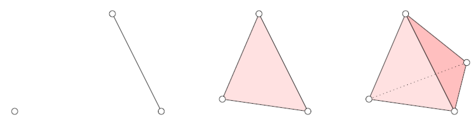
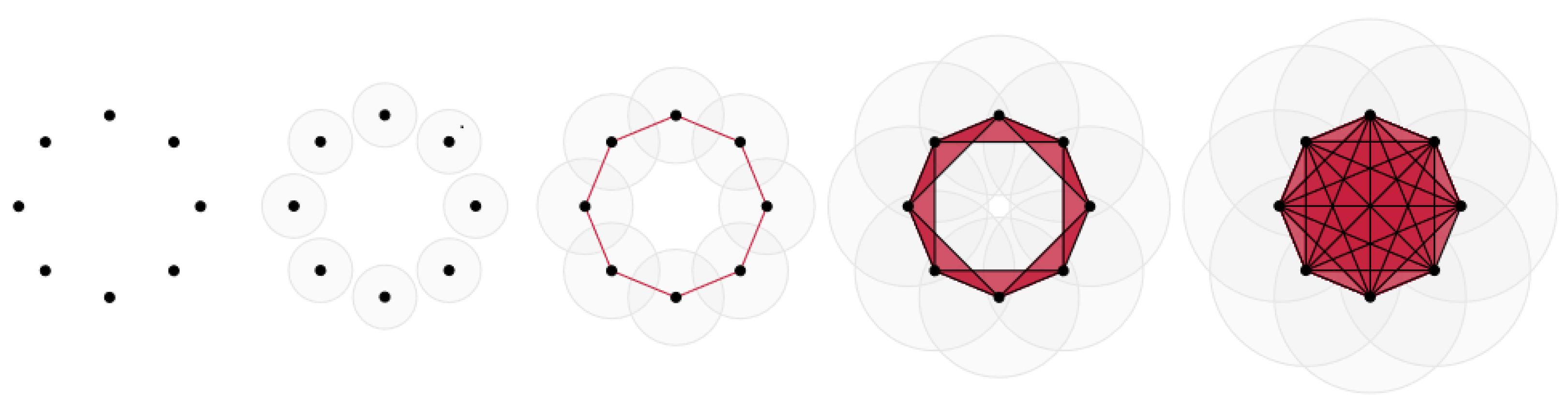
2.1. Simplicial Complexes

The smallest pieces from which we build upon are the simplices, as illustrated in Figure 1.

Definition 1.

Let $u_0,u_1,\dots ,u_k$ be points in ${\mathbb{R}}^d$. A k-simplex σ (or k-dimensional simplex) is the convex hull of $k+1$ affinely independent points. We denote $\sigma =[u_0,u_1,\dots ,u_k]$ the simplex spanned by the listed vertices. Its dimension is $dim\left(\sigma \right)=k$ and it has $k+1$ vertices.

A face of a simplex is the convex hull of an arbitrary subset of vertices of this simplex.

Under some conditions, several simplices put together can compose a greater structure called simplicial complex. The latter is very practical because it can be complex enough to approximate a more complex topological space, while it is composed by simple pieces (the simplices) which is beneficial for efficient computations. Examples of valid and non-valid geometric simplicial complexes are given in Figure 2.

Definition 2.

A (geometric) simplicial complex K is a non-empty set of simplices respecting the following conditions:

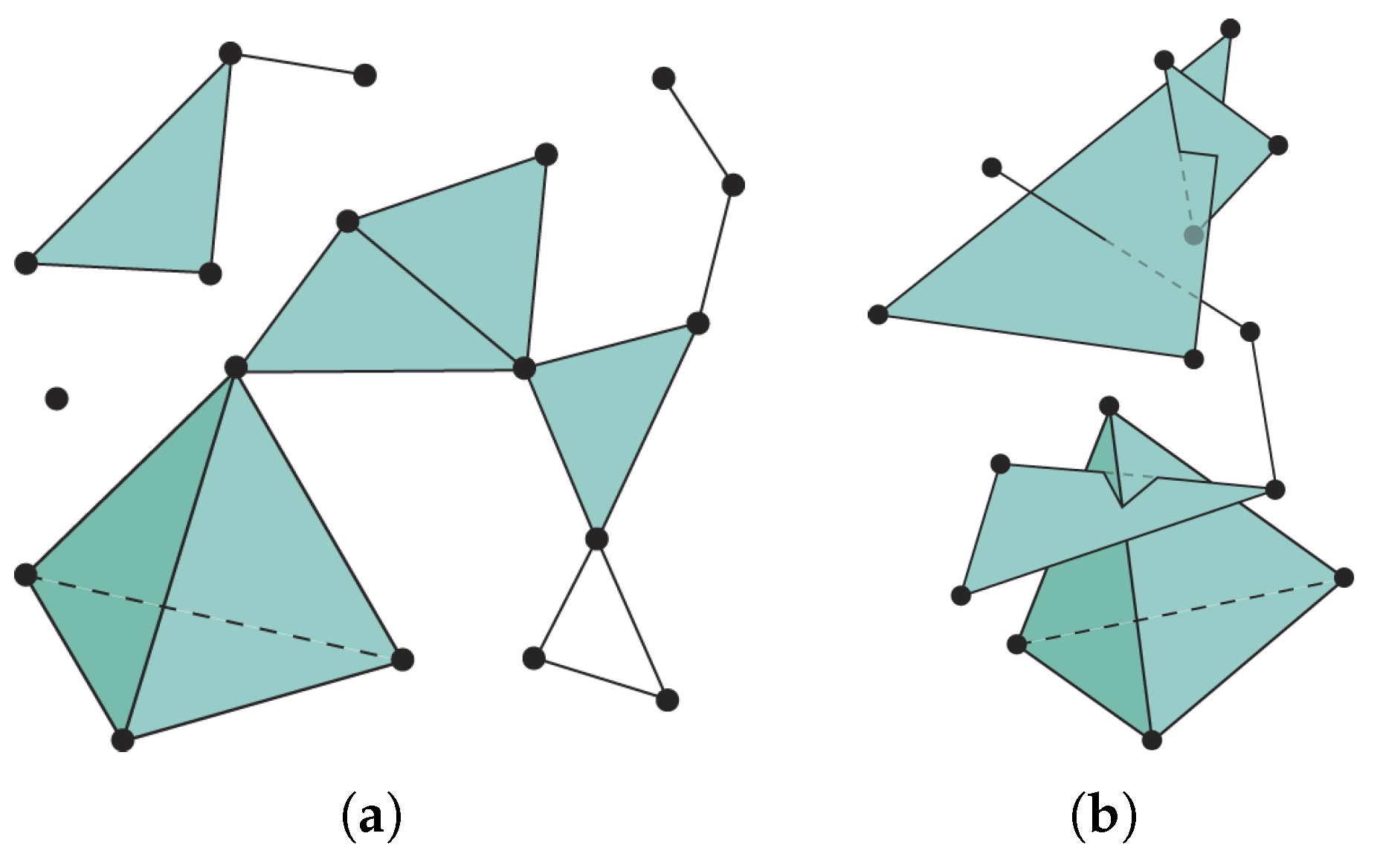
• Each face of any simplex of K is also a simplex of K.
• The intersection of any two simplices of K is either empty or a face of both simplices.

The dimension of K is the maximum dimension of any of its simplices. The underlying topological space is denoted $\left|K\right|$ and is the union of its simplices together with the induced topology (the open sets of ${\mathbb{R}}^d$) inherited from the ambient Euclidian space in which the simplices belong.

Now, we introduce the simplicial map which is a key notion used for the simplicial regularization of our Witness Simplicial VAE method.

Definition 3.

A simplicial map $f:K\to L$ between simplicial complexes K and L is a function $f:\mathit{Vert}K\to \mathit{Vert}L$ from the vertex set of K to that of L, such that, if $[u_0,u_1,\dots ,u_q]$ span a simplex of K then $[f\left(u_0\right),f\left(u_1\right),\dots ,f\left(u_q\right)]$ span also a simplex of L.

It is important to note here that a simplicial map f between two simplicial complexes K and L induces a continuous map $\tilde{f}$ between the underlying topological spaces $\left|K\right|$ and $\left|L\right|$. Indeed, for all points x in $\left|K\right|$, because x belongs to the interior of exactly one simplex in K, we can express this simplex by $[u_0,\dots ,u_q]$ using its vertices and x can be written as $x={\sum }_{i=0}^q{\lambda }_i{u}_i\mathrm{with}({\lambda }_0,\dots ,{\lambda }_q)\in {\mathbb{R}}_{+}^q\mathrm{such}\mathrm{that}{\sum }_{i=0}^q{\lambda }_i=1$. With these notations, the continuous map $\tilde{f}$ induced by the simplicial map f can be defined as: $\tilde{f}:x\mapsto \tilde{f}\left(x\right)=\tilde{f}\left({\sum }_{i=0}^q{\lambda }_i{u}_i\right)={\sum }_{i=0}^q{\lambda }_{i}f\left(u_i\right)$. It follows that the induced continuous map $\tilde{f}$ is completely determined by f so $\tilde{f}$ and f can actually be identified. The reader can refer to “Section 5: Simplicial Complexes” of the course [10] for the proofs of the continuity of this induced continuous simplicial map. Finally, we can highlight here that a simplicial map between two simplicial complexes is a linear map on the simplices.

If we think about the topology of a dataset, we can notice that usually not all the points are needed to know the underlying topology. Moreover, constructing simplices from just a subset of the data points is less computationally expensive than considering the whole dataset. These ideas motivated Vin de Silva and Gunnar Carlsson when they introduced the witness complex in [11]: a subset of the data points, called the landmarks points, is used to construct the simplices “seen” by the witnesses which are the rest of the points of the dataset. (The reader is invited to look at the mentioned paper [11] for a complete view on witness complexes, because here we make some simplifications and define the witness complex as a particular case of the original definition.)

Definition 4.

Let S be a finite set of points in ${\mathbb{R}}^d$ and write $B_r\left(x\right)$ for the closed d-dimensional ball with centre $x\in {\mathbb{R}}^d$ and radius $r\in \mathbb{R}$. Let $L\subset S$ be a subset of the points in S, that we call the landmarks. We define the witness complex of S, L, and $r\in \mathbb{R}$ as:

${\mathrm{W}}_r(S,L)=\left\{\sigma =[u_0,\dots ,u_k]\mathit{with}\{u_0,\dots ,u_k\}\subset L|\exists w\in Ss.t.\forall i\in ⟦0;k⟧,u_i\in B_r\left(w\right)\right\}.$

An example of the construction of a witness complex is given in Figure 3 and we explain it here:

On the left, we can see the 11 points with the landmarks points in green. The landmarks points are chosen arbitrarily here. Then, for a given radius r we check if any of the balls (here the 2-dimensional balls are disks) centred at the points of S contains a set of landmarks. In that case the centre of the disk is called a witness (encircled in red), and the set of the corresponding landmarks points form a simplex which is added to ${\mathrm{W}}_r(S,L)$. Here only the balls around the witnesses are represented.

On the top right in blue, we can see a simplicial complex built by joining all the points. It is actually the 1-nearest neighbour graph and consists of 11 0-simplices (all the points of the dataset), and 11 1-simplices (the edges). On the bottom right in green, we can see the Witness complex ${\mathrm{W}}_r(S,L)$ constructed as explained above. This one consists of five 0-simplices (the landmarks points), six 1-simplices (the edges), and one 2-simplex (the triangle).

As we see in this example of Figure 3, it is important to note that the witness complex, although being composed of simplices corresponding to vertex sets of only a subset of landmarks points $L\subset S$, can still capture the topology of the whole dataset S. However, this is true in this example but it may not be always the case and it mainly depends on the choice of the landmarks L and the radius r. In order to construct a witness complex, the landmarks can be chosen for example arbitrarily or randomly (another method called “maxmin” is also given in [11] to select the landmarks in an iterative way). Regarding the choice of the radius r, this is addressed below when we mention the concept of filtration used in persistent homology.

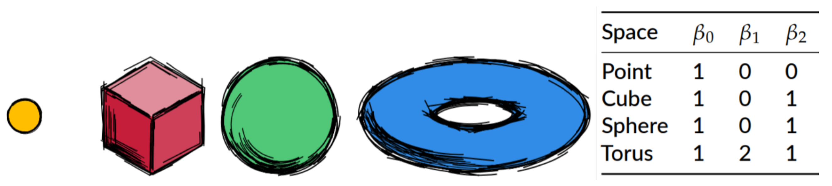
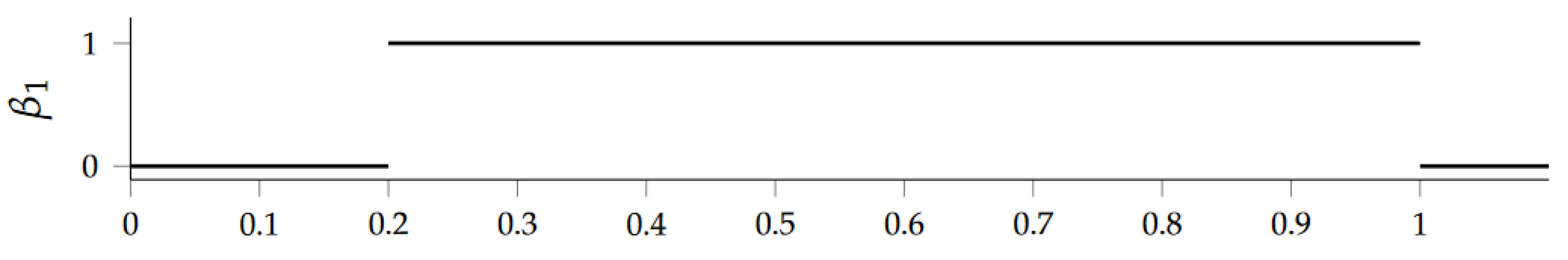
2.2. Betti Numbers

A topologist is interested in classifying different objects (topological spaces to be more precise) according to their shape. Two objects are topologically equivalent if there exists a homemorphism between them, that is a continuous map with continuous inverse. Algebraic topology provides the mathematical theory for such classification thanks to algebraic topological invariants. As suggested by their name, the latter do not change between topologically equivalent spaces. Computational topology allows us to compute efficiently such topological invariants, in particular with the help of previously defined notions of simplicial complexes. Examples of algebraic topological invariants in which we are interested are the Betti numbers. We give here the intuition, for the mathematical formalism (rank of the p-th homology group etc.) the reader is invited to look at the references mentioned in the introduction of this section.

We can say that the p-th Betti number, denoted ${\beta }_p$, counts the number of p-dimensional holes: ${\beta }_0$ is the number of connected components, ${\beta }_1$ the number of tunnels, ${\beta }_2$ the number of voids, etc. It is indeed a topological invariant and one can intuitively notice that the Betti numbers of an object do not change when we deform this object continuously, such as changing its scale. Thus, they can be used to classify objects of different topologies. For a topologist, a sphere and the surface of a cube are identified to be the same object and their Betti numbers are equal, but the torus is different since it has a different topological structure. This is illustrated in Figure 4.

When it comes to analysing data, since the latter is usually discrete and represented as points in a space, we need to take into account the different possible topologies of a dataset across different scales. This leads us to the concept of filtration in persistent homology. We illustrate this notion in Figure 5 through a simple example where the data are a set of 8 points sampled from a circle in a 2-dimensional space. This is a simple example of a “(Vietoris–Rips) filtration” where we can see that the values of the Betti numbers ${\beta }_0$ and ${\beta }_1$ change depending on the scale from which we consider the data. We can wonder which scale, and, thus, which values of the Betti numbers, is appropriate to describe the topology of this dataset. Persistent homology aims to answer to this question through this notion of filtration.

As illustrated in the above Figure 5, for the simplices of dimension 1 (the edges) and simplices of dimension 2 (the triangles), the process of the “(Vietoris–Rips) filtration” is as follows: around each point we draw disks of a growing diameter $ϵ$ (from left to right in Figure 5 the diameter $ϵ$ is increasing), as soon as two disks have a common non-empty intersection we draw an edge between their centre, and as soon as three centres form a triangle with the drawn edges then we draw the triangle. Finally, we look at the Betti numbers at each step of the filtration depending on the scale $ϵ$. In this example of Figure 5, we can see that ${\beta }_0$, which counts the number of connected components, is decreasing from 8 to 1 when $ϵ$ increases. For ${\beta }_1$, which counts the number of 1-dimensional holes, it is different: it goes from 0 to 1 and to 0 again while $ϵ$ is increasing. The values of ${\beta }_1$ in function of $ϵ$ are represented in the barcode given in Figure 6. When $ϵ$ is equal to 1, the drawn edges form a fully connected graph and ${\beta }_0$ and ${\beta }_1$ will not vary anymore. Then we can look at this barcode for $ϵ$ between 0 and 1, and see the values of ${\beta }_1$ which persist the most. In this case the “persistent ${\beta }_1$” is ${\beta }_1=1$ since it persists between $ϵ=0.2$ and $ϵ=1$. Indeed, for this interval of $ϵ\in [0.2;0.5]$, we can recognize the circle from which the points were sampled: the drawn edges or triangles all together form an object with one 1-dimensional hole, which is topologically equivalent to a circle since we can deform continuously this object to obtain a circle.

All the information present in a barcode can be equivalently represented in a persistence diagram where the birth and death of different classes can also be visualised. Finally, the witness complex filtration is a similar concept than Vietoris–Rips filtration presented above, except that we consider a witness complex. What that means is that during the filtration, we increase the radius of the balls centred at the witnesses and we connect only the landmarks “seen” by a witness to form the simplices of the witness complex.

To conclude, the Betti numbers allow one to analyse and describe the topology of an object, and persistent homology leads to the notions of filtration and persistent Betti numbers to better analyse a dataset. Indeed, the filtration process provides a way to recover its underlying topological structure that can be approximated by a witness complex built with a radius corresponding to a persistent Betti number.

3. Related Work

3.1. Non-Linear Dimensionality Reduction

In order to analyse high dimensional data, it might be convenient to reduce its dimensionality, in particular for visualization. The traditional methods were based on linear models, the well-known archetype being the principal component analysis [13,14]. However, by construction these methods are not efficient to reduce highly non-linear data without losing too much important information. That is why, to deal with complex datasets, non-linear dimensionality reduction methods were developed, this field is known as “manifold learning”. An overview of such methods with their advantages and drawbacks is given in [15]. We introduce in this section some famous non-linear dimensionality reduction methods, among them the ones that inspired us for our work.

A classical non-linear dimensionality reduction method is Isomap (from isometric mapping) which was introduced in 2000 by Tenenbaum et al. [16]. It maps points of a high-dimensional non-linear manifold to a lower dimensional space by preserving graph distances. In particular, it consists first of constructing a graph on the manifold of the data considering points which are neighbours regarding some euclidean distance (i.e., the euclidean distance between two neighbouring points should be smaller than a threshold, or an alternative is to apply a k-nearest neighbours algorithm). Then, the shortest path on the graph between any pair of points is computed using for example Dijkstra’s algorithm. This gives an approximation of the geodesic distance between any pair of points. Finally, the classical multidimensional scaling (MDS) method (see [17,18,19] for references) is applied to the matrix of graph distances in order to embed the data in a smaller dimensional space while preserving these approximated geodesic distances. The advantage of this method is that the geometry of the manifold is generally well preserved under some hypothesis (for some class of manifolds, namely the “developable manifolds” [15]). However, the drawbacks is the costly computation of the (approximated) geodesic distances.

Another famous method used in data visualization is t-SNE [20] which allows one to perform non-linear dimensionality reduction. It was developed in 2008 by van der Maaten and Hinton as a variation of Stochastic Neighbour Embedding [21]. t-SNE aims to better capture global structure, in addition to the local geometry, than previous non-linear dimensionality reduction techniques for high dimensional real world datasets. It is also based on pairwise similarities preservation between the input data space and the embedding. The particularity of this method is that it starts by converting Euclidean pairwise distances into conditional probabilities using Gaussian distributions, that is the similarity of a point to a given point is the conditional probability of being its neighbour under a Gaussian distribution centred at the given point. For the embedding lower dimensional space, the pairwise similarity is constructed in an analogue way except that the authors of [20] use a Student t-distribution instead of a Gaussian. They actually consider the joint probabilities defined as being the symmetrized conditional probabilities. Then, they minimize the Kullback–Leiber divergence between the joint probability distribution of the input data space and the one of the embedding.

UMAP (Uniform Manifold Approximation and Projection) is a more recent non-linear dimensionality reduction method developed in 2018 by McInnes, Healy, and Melville [22]. It is based on three assumptions about the data: it should be uniformly distributed on a Riemannian manifold, the Riemannian metric should be approximated as locally constant, and the manifold should be locally connected. The first step of the method is to construct a fuzzy simplicial complex of the data, which is a simplicial complex with probabilities assigned to each simplex. Then, the data are embedded in a lower dimensional space by minimizing an error function (namely the fuzzy set cross entropy [22]) between the fuzzy topological structures of the original data and the embedded data, through a stochastic gradient descent algorithm. Like with Isomap, varying the parameters of the method allows us to choose if we want to preserve more global versus local structure of the data. The advantages of UMAP are that it is scalable to high dimensional datasets and it is fast. Drawbacks might be that there are two parameters to tune, and that the relative distances between different clusters of a UMAP embedding are meaningless.

3.2. Variational Auto-Encoder

The variational auto-encoder (VAE) not only allows us to do non-linear dimensionality reduction, but it has also the particularity to be a generative model. It was simultaneously discovered in 2014 by Kingma and Welling in [2] and Rezende, Mohamed, and Wierstra in [3]. Although it could be seen as a stochastic version of the well known auto-encoder, the motivation behind the VAE is completely different since it comes from Bayesian inference. Indeed, the VAE has a generative model and a recognition model or inference model, and both are Bayesian networks. The original papers cited above provide a method using stochastic gradient descent to learn jointly latent variable models whose distributions are parameterized by neural networks and corresponding inference models. The VAE can be used for many different applications such as generative modelling, semi-supervised learning, representation learning, etc. We refer the reader to the recent introduction to VAEs made by Kingma and Welling in [23] for more complete details.

Following the notations of [2], let $X={\left\{{\mathrm{x}}^{\left(i\right)}\right\}}_{i=1}^N$ be the dataset consisting of N i.i.d. observed samples of some variable x, generated by a random process involving unobserved random variables z called the latent variables. This process consists of two steps: generation of latent variables from a prior distribution $p_{{\theta }^{*}}\left(z\right)$ (the prior), and generation of the observed variables from a conditional distribution $p_{{\theta }^{*}}\left(x\right|z)$ (the likelihood); the true parameters ${\theta }^{*}$ and the latent variables are unknown. We assume that the prior and the likelihood are parameterized by $\theta$ and their probability distribution functions are almost everywhere differentiable. ${\theta }^{*}$ is the optimal set of parameters $\theta$ maximizing the probability of generating real data samples ${\mathrm{x}}^{\left(i\right)}$. Additionally, the true posterior density $p_{\theta }\left(z\right|x)$ is assumed to be intractable. That is why Kingma and Welling [2] introduced a recognition model $q_{\varphi }\left(z\right|x)$ parameterized by $\varphi$ to approximate the true posterior $p_{\theta }\left(z\right|x)$. The latent variables z, also called “code”, are latent representations of the data. $q_{\varphi }\left(z\right|x)$ is then called the probabilistic “encoder” because it gives a probability distribution of the latent variables from which the data X could have been generated. This leads us to $p_{\theta }\left(x\right|z)$ which is called the probabilistic “decoder” because it gives a probability distribution of the data x conditioned on a latent representation z. In our case, $\theta$ and $\varphi$ are parameters of artificial neural networks, and the method presented in [2] allows the model to jointly learn $\theta$ and $\varphi$. On one side, the encoder learns to perform non-linear dimensionality reduction if we take, for the latent representations z, a lower dimension than the original data. On the other side, the decoder allows us to do generative modelling in order to create new realistic data from latent representations.

As it is typically done in variational Bayesian methods, a good generative model should maximize the “log-evidence” which is here the marginal log-likelihood $log{p}_{\theta }\left(x\right)$. The latter is intractable and we have $log{p}_{\theta }\left(x\right)={\mathcal{L}}_{\theta ,\varphi }\left(x\right)+D_{KL}(q_{\varphi }\left(z\right|x)\left|\right|p_{\theta }\left(z\right|x))$ with ${\mathcal{L}}_{\theta ,\varphi }\left(x\right)={\mathbb{E}}_{q_{\varphi }\left(z\right|x)}log\frac{p_{\theta }(x,z)}{q_{\varphi }\left(z\right|x)}$ the ELBO (evidence lower bound or variational lower bound) and $D_{KL}(q_{\varphi }\left(z\right|x)\left|\right|p_{\theta }\left(z\right|x))={\mathbb{E}}_{q_{\varphi }\left(z\right|x)}log\frac{q_{\varphi }\left(z\right|x)}{p_{\theta }\left(z\right|x)}$ the Kullback–Leibler (KL) divergence between $q_{\varphi }\left(z\right|x)$ and $p_{\theta }\left(z\right|x)$ (see Appendix A.1 for the derivation). The ELBO is indeed a lower bound of the marginal log-likelihood (${\mathcal{L}}_{\theta ,\varphi }\left(x\right)\le p_{\theta }\left(x\right)$), and maximizing it allows us to (1) approximately maximize $p_{\theta }\left(x\right)$ to obtain a better generative model, and (2) minimize the KL divergence to obtain a better approximation $q_{\varphi }\left(z\right|x)$ of the intractable true posterior $p_{\theta }\left(z\right|x)$. Hopefully, the ELBO can be explicited (see Appendix A.2 for the derivation) and is actually the objective function of the VAE:

$${\mathcal{L}}_{VAE}={\mathcal{L}}_{\theta ,\varphi }\left(x\right)={\mathbb{E}}_{q_{\varphi }\left(z\right|x)}log{p}_{\theta }\left(x\right|z)-D_{KL}(q_{\varphi }\left(z\right|x)\left|\right|p_{\theta }\left(z\right))$$

(1)

Equation (1) shows that the loss of the VAE can be computed through the expected reconstruction error ${\mathbb{E}}_{q_{\varphi }\left(z\right|x)}log{p}_{\theta }\left(x\right|z)$, and the KL divergence between the encoder $q_{\varphi }\left(z\right|x)$ and the prior $p_{\theta }\left(z\right)$. Typically, the terms in the KL divergence are chosen as Gaussians so that it can be integrated analytically. Otherwise, if the integration is not possible we can do a Monte Carlo estimation. Finally, it was introduced the “reparameterization trick” (Kingma and Welling [2], and Rezende et al. [3]) to efficiently optimize the objective function ${\mathcal{L}}_{\theta ,\varphi }\left(x\right)$ with respect to the parameters $\theta$ and $\varphi$ using stochastic gradient descent.

3.3. Topology and Auto-Encoders

The use of topology in machine learning is quite new with the development of topological data analysis. Some recent work, such as the “topology layer” proposed by Gabrielsson et al. [24], focus on preserving the topology of single inputs which can be cloud points or images. However, we want to preserve the topology of the whole dataset between the input and the latent space, and particularly in a variational auto-encoder framework. The ability of a standard auto-encoder to preserve the topology for datasets composed by rotations of images was investigated by Polianskii [25]. We are now interested in an active control of the topology instead of a passive analysis. The main difficulty is that algebraic topological invariants, such as the Betti numbers, are discrete whereas we need some differentiable function with respect to the neural network parameters in order to be able to perform backpropagation of the gradient. At the time we were working on this problem, to the best of our knowledge, no previous work was made in the direction of adding to the loss of a VAE a term to preserve the topology except in the appendix of [26], where the authors Moor et al. sketched an extension of their topological auto-encoder to a variational setup. Their topological auto-encoder presents in the loss a differentiable topological constraint term added to the reconstruction error of an auto-encoder. Although this method is generalizable to higher order topological features, they focused on preserving 0-homology. Through persistent homology calculation using the Vietoris–Rips complex, their topological constraint aims to align and preserve topologically relevant distances between the input and the latent space. The authors present this “topological loss” as a more generic version than the “connectivity loss” proposed by Hofer et al. [27]. Although the connectivity loss is also obtained by computing persistent 0-homology of mini-batches, on the contrary to the topological loss it operates directly on the latent space of an auto-encoder to enforce a single scale connectivity through a parameter denoted $\eta$ [27].

Another interesting approach combining topology and Auto-Encoders is the “simplicial regularization” introduced recently by Gallego-Posada [28,29] as a generalization of the “mixup” regularization ([30,31]). Gallego-Posada in his master thesis [28] applies UMAP to the data and computes the Fuzzy simplicial complexes of both the input data and the embedding, and uses these simplicial complexes to compute simplicial regularizations of both the encoder and the decoder, that he adds to the auto-encoder loss. The simplicial regularizations aim to “force” the encoder and the decoder to be simplical maps, that is to be linear over the simplices. We wanted to explore this idea in a variational setup with our Witness Simplical VAE (see Section 7 for the proposed method) which uses similar simplicial regularizations but computed using a witness complex. The latter simplicial complex was introduced by De Silva and Carlsson [11] and allows one to obtain a topological approximation of the data with a small number of simplices. Lastly, we can mention that the idea of using such witness complex came from the “geometry score” developed by Khrulkov and Oseledets [32], which is a method for evaluating a generative model by comparing the topology of the underlying manifold of generated samples with the original data manifold through the computation of witness complexes.

Finally, we can mention a completely different approach aiming to capture geometric and topological structure with a VAE that is by having a latent space which is a specific Riemannian manifold instead of an Euclidean space. In this direction Pérez Rey et al. proposed the Diffusion VAE [33] which allows one to choose an arbitrary Riemannian manifold as a latent space, such as a sphere or a torus, for example. However, this approach implies a strong inductive bias on the geometric and topological structure of the data.

4. Implementation Details

Regarding the implementation we used PyTorch for fast tensor computing via graphics processing units (GPU) and for automatic differentiation of the objective function of the neural networks [34]. In particular, we used the Adam algorithm [35] (with, by default, a learning rate parameter equal to ${10}^{-3}$) provided with PyTorch for the stochastic optimization of the objective function. The implementation for the witness complex construction uses the code from [36] built on top of the GUDHI library [37] for the provided simplex tree data structure [38].

All the code is publicly available at (accessed on 29 December 2022): https://github.com/anissmedbouhi/master-thesis.

5. Problem Formulation

Our research question can be summarized as follows: how to preserve the topology of data between the input and the latent spaces of a variational auto-encoder?

We particularly focus on preserving the persistent Betti numbers which are topological invariants. Indeed, although all the topological information is not contained in the persistent Betti numbers, they do provide relevant information regarding the topological structure of the data. Our goal is thus to have a VAE, such that the persistent Betti numbers are equal, between the input data, its latent representation given by the encoder, and ideally also its reconstruction given by the decoder.

After showing that this is not the case for a vanilla VAE, we modify the loss of the VAE in order to encourage such preservation. Since we focus on a 2-dimensional latent space, we can directly evaluate visually if this goal is achieved for the two first persistent Betti numbers, namely ${\beta }_0$ and ${\beta }_1$, without needing to compute the persistent diagrams. In summary, for the two datasets we consider, our goal is to preserve both 0-homology and 1-homology.

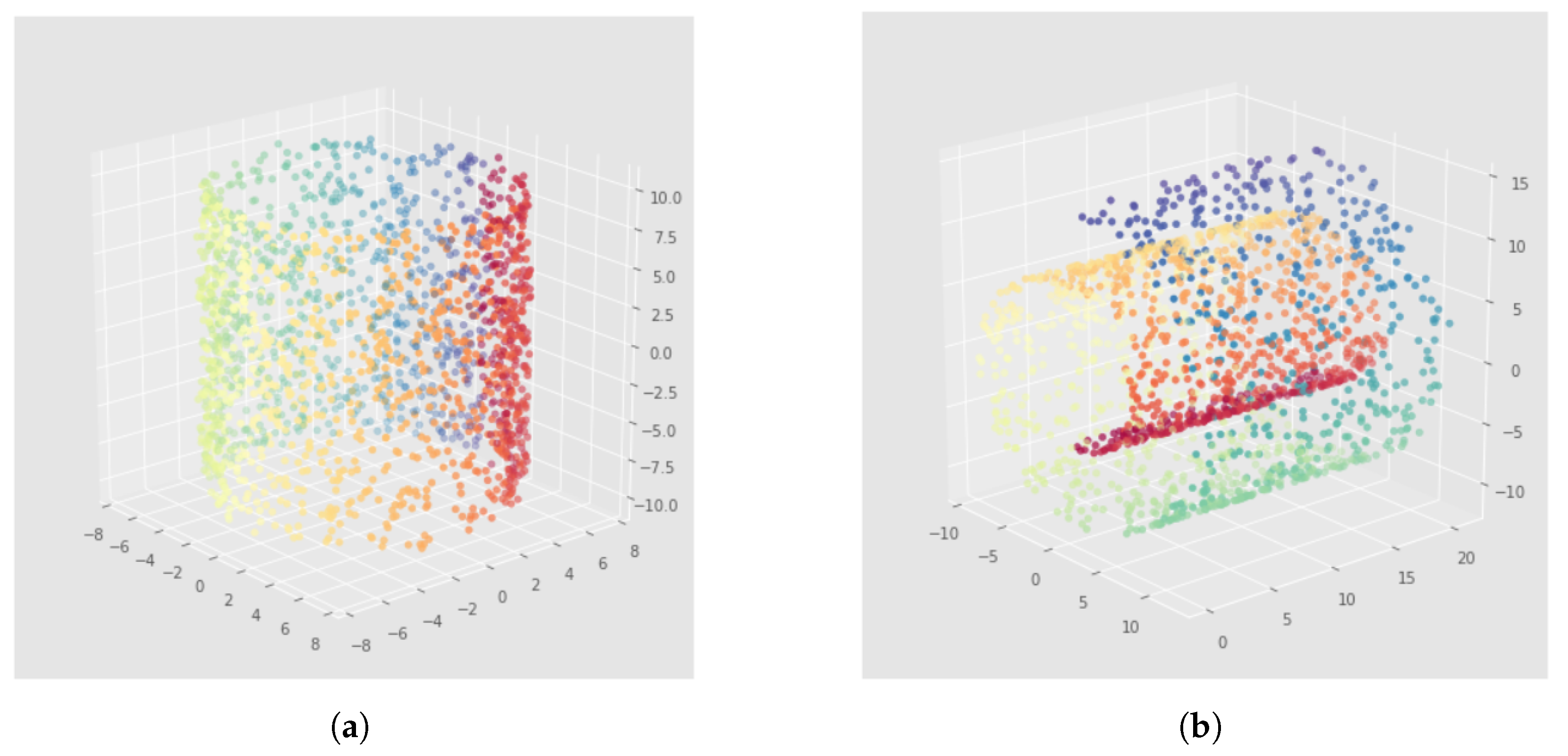
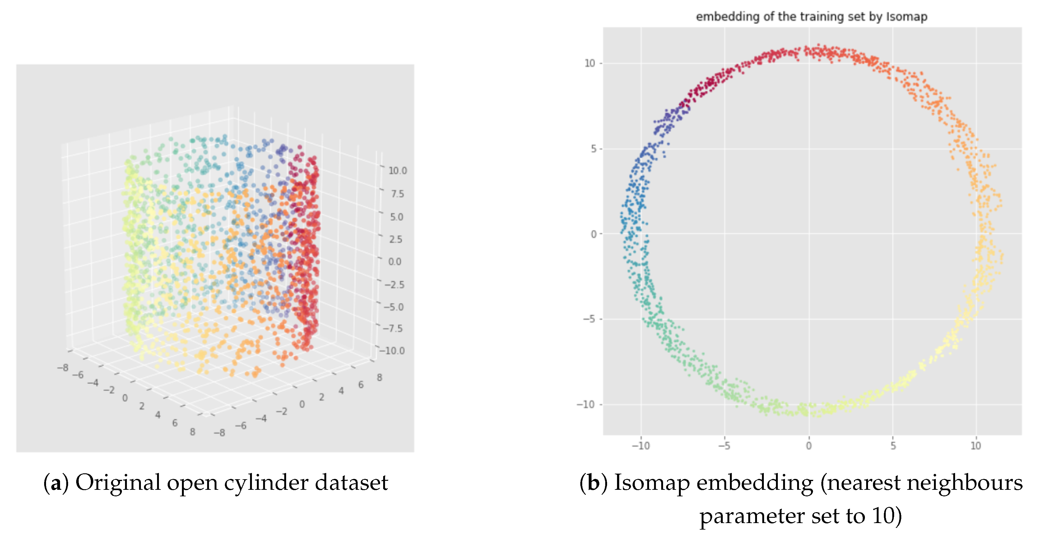
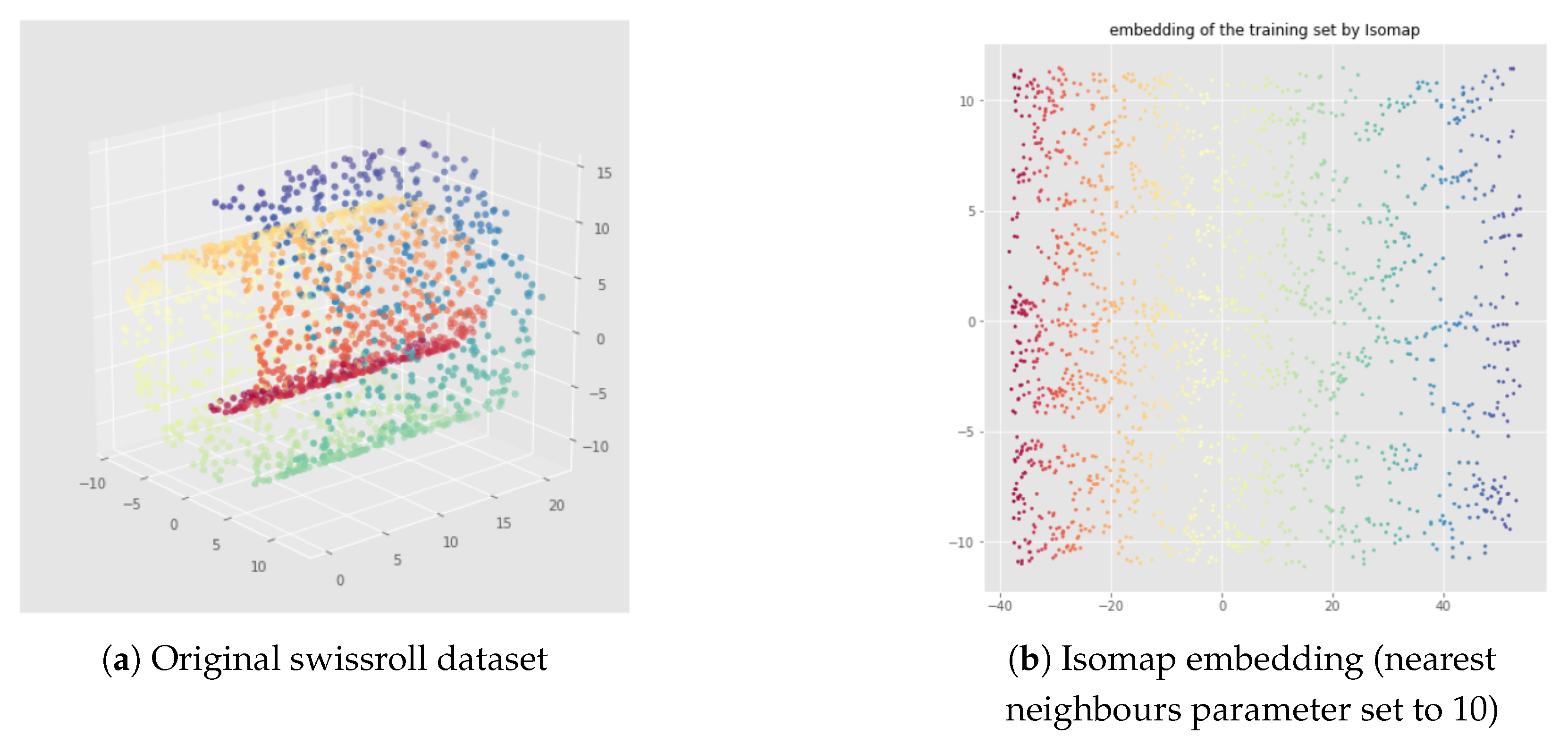
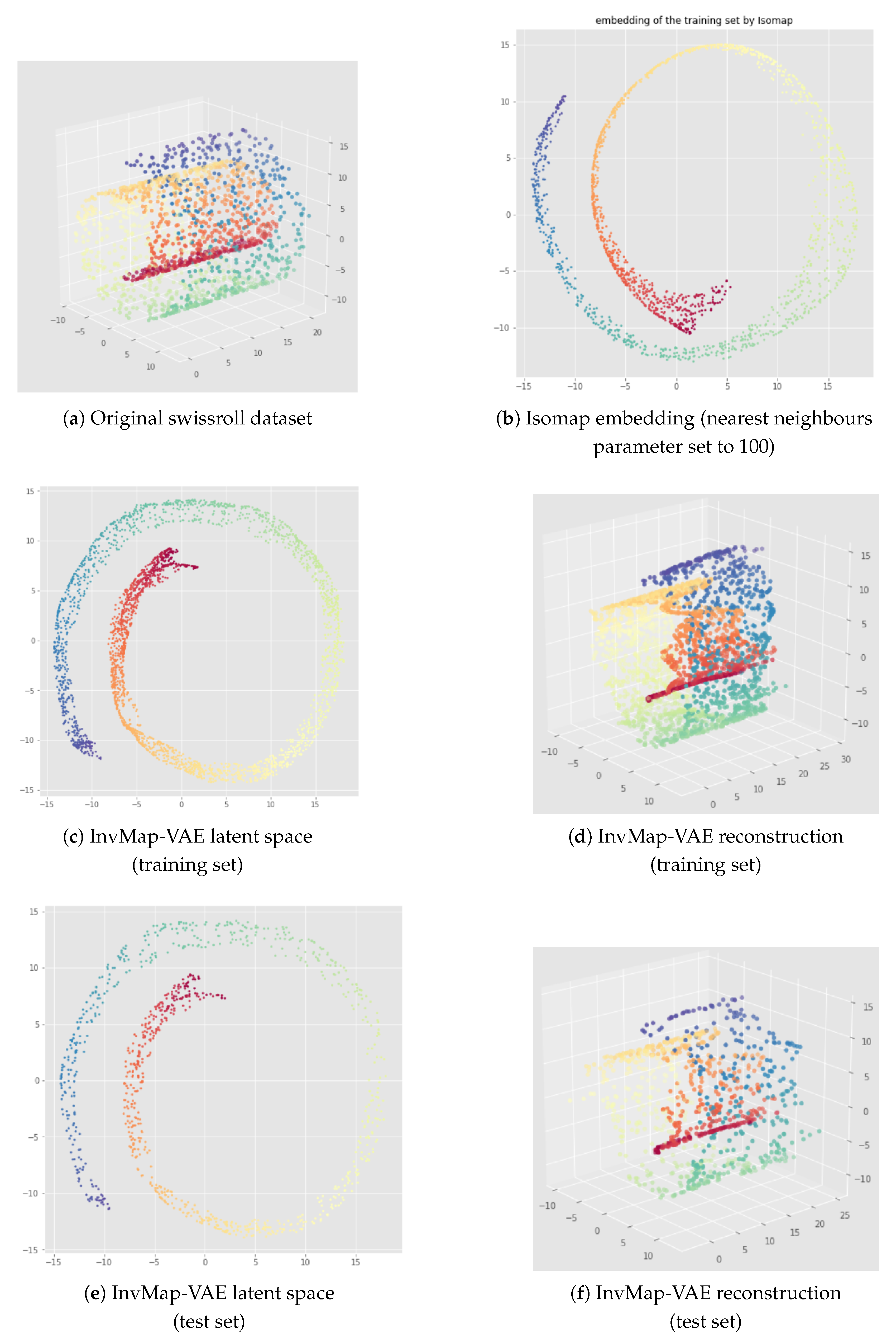
5.1. Datasets

For the purpose of our problem, we focus on two synthetic datasets with interesting geometry and topology, embedded in three dimensions. We reduce their dimension to a 2-dimensional latent space to visualize directly the impact of our methods. We call the two datasets we used the open cylinder and the swissroll as illustrated in Figure 7. For both, we sampled 5000 points: 60% for training, 20% for validation, and 20% for testing.

To generate the points $(x,y,z)\in {\mathbb{R}}^3$ of the open cylinder, we sampled from uniform distributions: $z\sim {\mathcal{U}}_{[-h/2,h/2]}$; $r\sim {\mathcal{U}}_{[r-w/2,r+w/2]}$; $\theta \sim {\mathcal{U}}_{[0,2\pi ]}$; with h for “height”, r for “radius”, and w for “width”; and then we define $x=rsin\theta$, $y=rcos\theta$ and $z=z$. For this open cylinder we used the following parameters: 20 for the height, 1 for the width, and 7 for the radius.

For the swissroll, its points $(x,y,z)\in {\mathbb{R}}^3$ were generated with scikit-learn [39] using an algorithm from [40]. It also works with sampling from uniform distributions: $t\sim 1.5{\mathcal{U}}_{[\pi ,3\pi ]}$; $y\sim 21{\mathcal{U}}_{[0,1]}$; and then are defined $x=tcost$, $y=y$ and $z=tsint$.

As we can visualize in Figure 7, since ${\beta }_0$ counts the number of connected components and ${\beta }_1$ the number of 1-dimensional holes, we can say that ${\beta }_0^{\mathrm{OpenCylinder}}={\beta }_0^{\mathrm{Swissroll}}={\beta }_1^{\mathrm{OpenCylinder}}=1$ and ${\beta }_1^{\mathrm{Swissroll}}=0$. The goal is to preserve these persistent Betti numbers in the latent space of a VAE.

5.2. Illustration of the Problem

In this section, we present some results obtained with a standard VAE to illustrate the problem and to have a baseline with which we can compare the methods. By “standard VAE” we mean a VAE with a Gaussian prior which has a standard loss that consists of the reconstruction and the KL-divergence terms.

Figure 8, Figure 9, Figure 10 and Figure 11 provide representative results of the standard VAE applied to the open cylinder dataset, for different random initializations (“pytorchseed”) of the neural network weights and a batch size equal to 128. We do not always show the losses since they look similar for different initializations, but it should be noted that after 500 epochs the learning process is always converging, like in Figure 8f. The trained VAEs perform similarly on both train and test data leading to the same conclusions. In the figures below, we show the results for the training sets for a better visualization due to larger point set size. We can see that for the standard VAE, there is not much consistency of the representation learning when the random initialization of the neural network weights is changed since the latent representations can appear in very different ways. Most of the time, we observe the first persistent Betti number as ${\beta }_1=0$, like in Figure 9, or ${\beta }_1=2$, like in Figure 8, instead of ${\beta }_1=1$ as it should be for the open cylinder. Sometimes, we can obtain ${\beta }_1=1$ but it is not satisfactory from the point of view of latent space interpolation: either because some regions may be separated (see Figure 10), or because the 1-dimensional hole in the latent representation does not really make sense and is not useful for interpolating in the latent space since the “color order” is not preserved (see Figure 11).

For the swissroll dataset, we also obtain completely different latent representations when the random initialization of the neural network weights is changed, as we can see in Figure 12, Figure 13 and Figure 14. Indeed, when different network initializations are used, we can have different persistent Betti numbers which are not the same as the original dataset, and we obtain similar discontinuity problems as for the examples of the open cylinder dataset.

Our testing concludes that in practice the standard VAE does not take the topology of data into account when it learns the latent representation of input data. Moreover, learnt embeddings are not consistent with respect to different weight initialization.

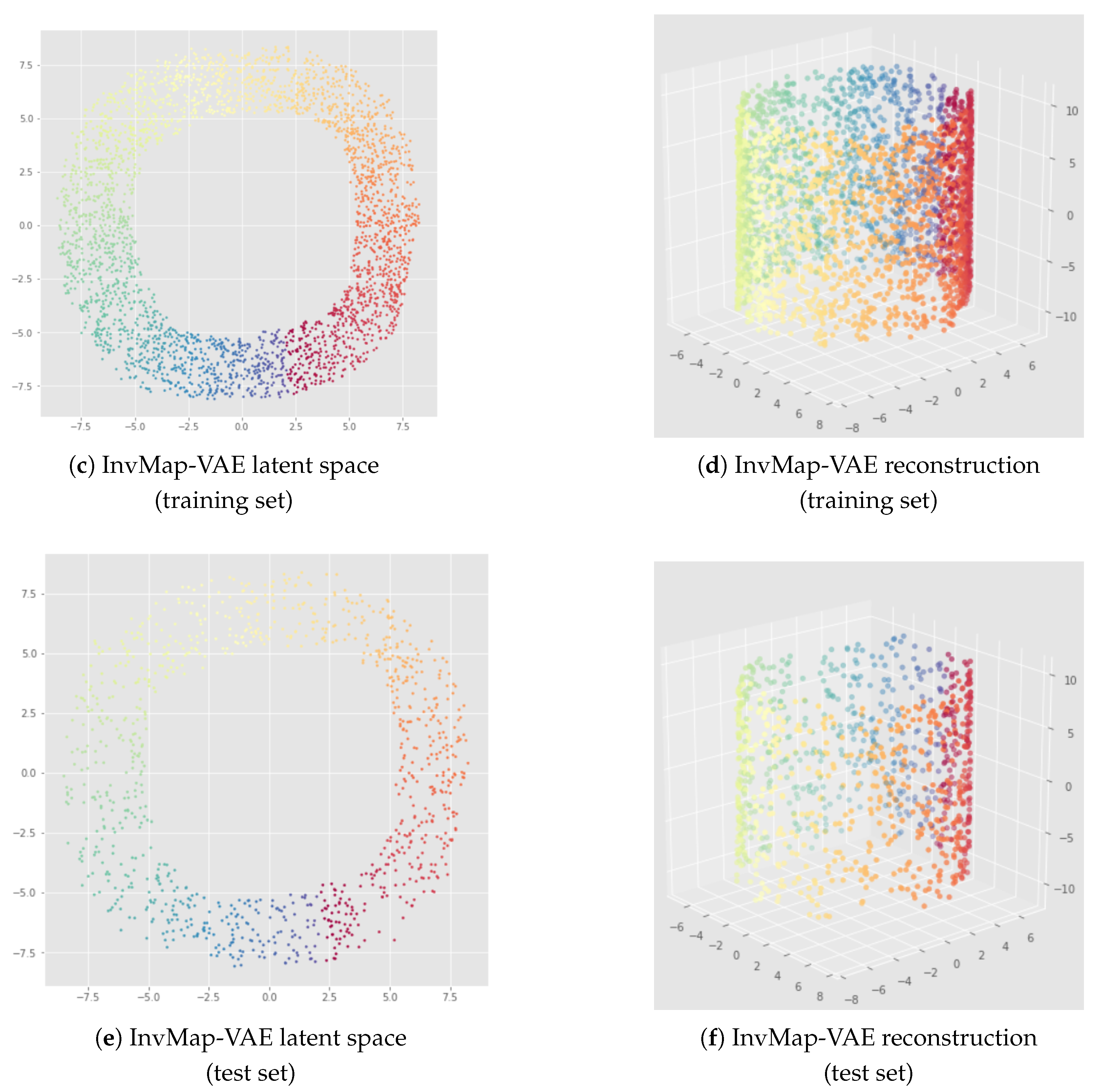
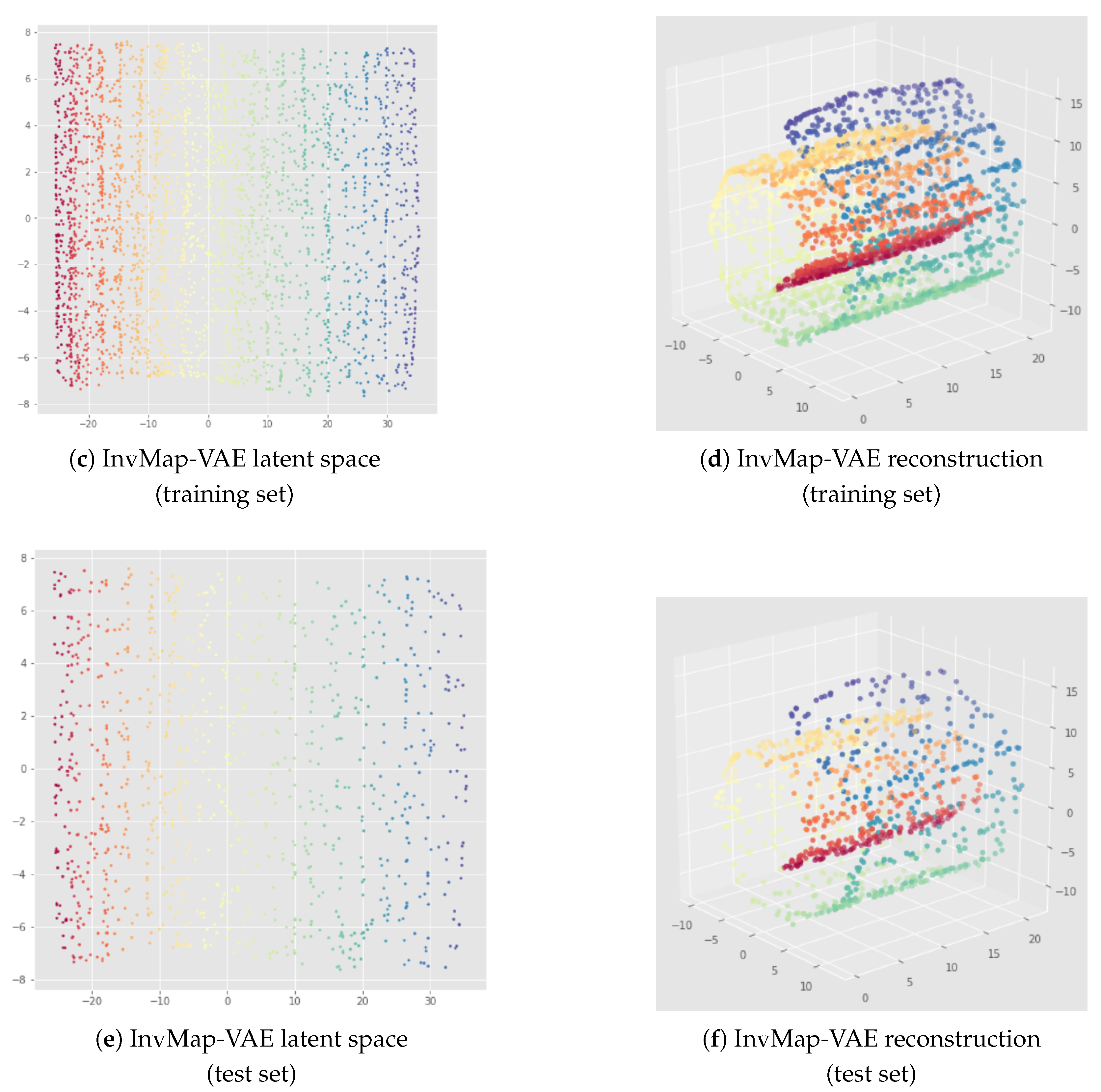
6. InvMap VAE

6.1. Method

Here, we propose our first method called InvMap-VAE. Given an embedding of the data, this method allows us to obtain a VAE with a latent representation that is geometrically and topologically similar to the given embedding. So this method depends on an embedding which can be given arbitrarily or by any dimensionality reduction technique. The main advantages of InvMap-VAE are that the learned encoder provides a continuous (probabilistic) mapping from the high dimensional data to a latent representation with a structure closed to the embedding, and the decoder provides the continuous inverse mapping, which are both lacking in manifold learning methods, such as Isomap, t-SNE, and UMAP. Below, we present the results of an Isomap-based InvMap-VAE, where we use an embedding provided by Isomap, although any other fitting dimensionality reduction technique could be used.

Let X be the original data, and $Z_{emb}$ the given embedding, for example obtained when applying a dimensionality reduction technique to X. Let us call Z the latent representation of a VAE applied to X. Then, to obtain the loss of the InvMap-VAE, we simply add to the VAE loss (see Equation (1) page 207), the Mean Square Error (MSE) between Z and $Z_{emb}$ multiplied by a weight denoted $w_{IM}$:

$${\mathcal{L}}_{InvMapVAE}={\mathcal{L}}_{VAE}+w_{IM}\times \mathrm{MSE}(Z,Z_{emb})$$

(2)

In practice, we compute this loss on a batch level as it is performed with the Standard VAE to perform “batch gradient descent” [23].

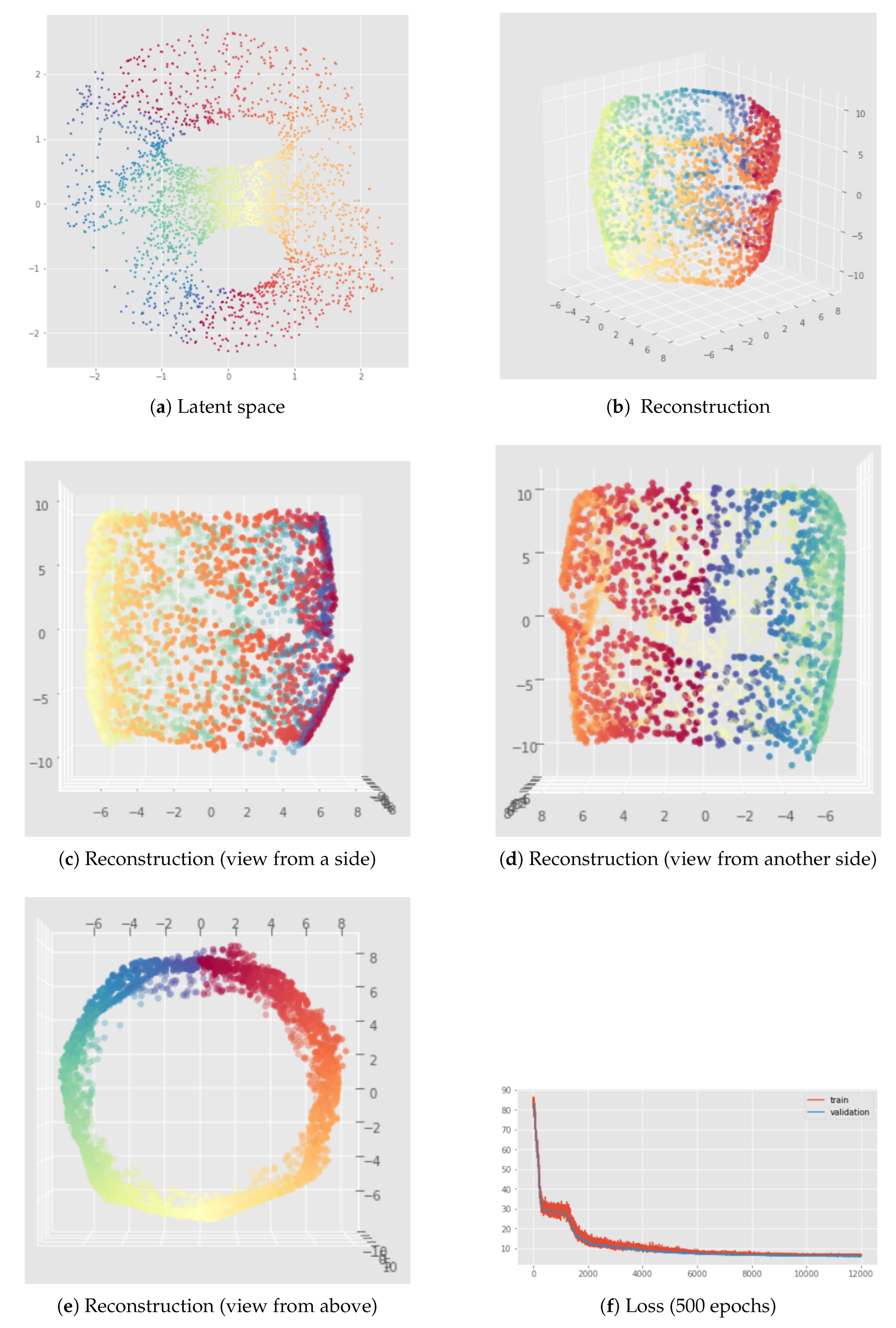
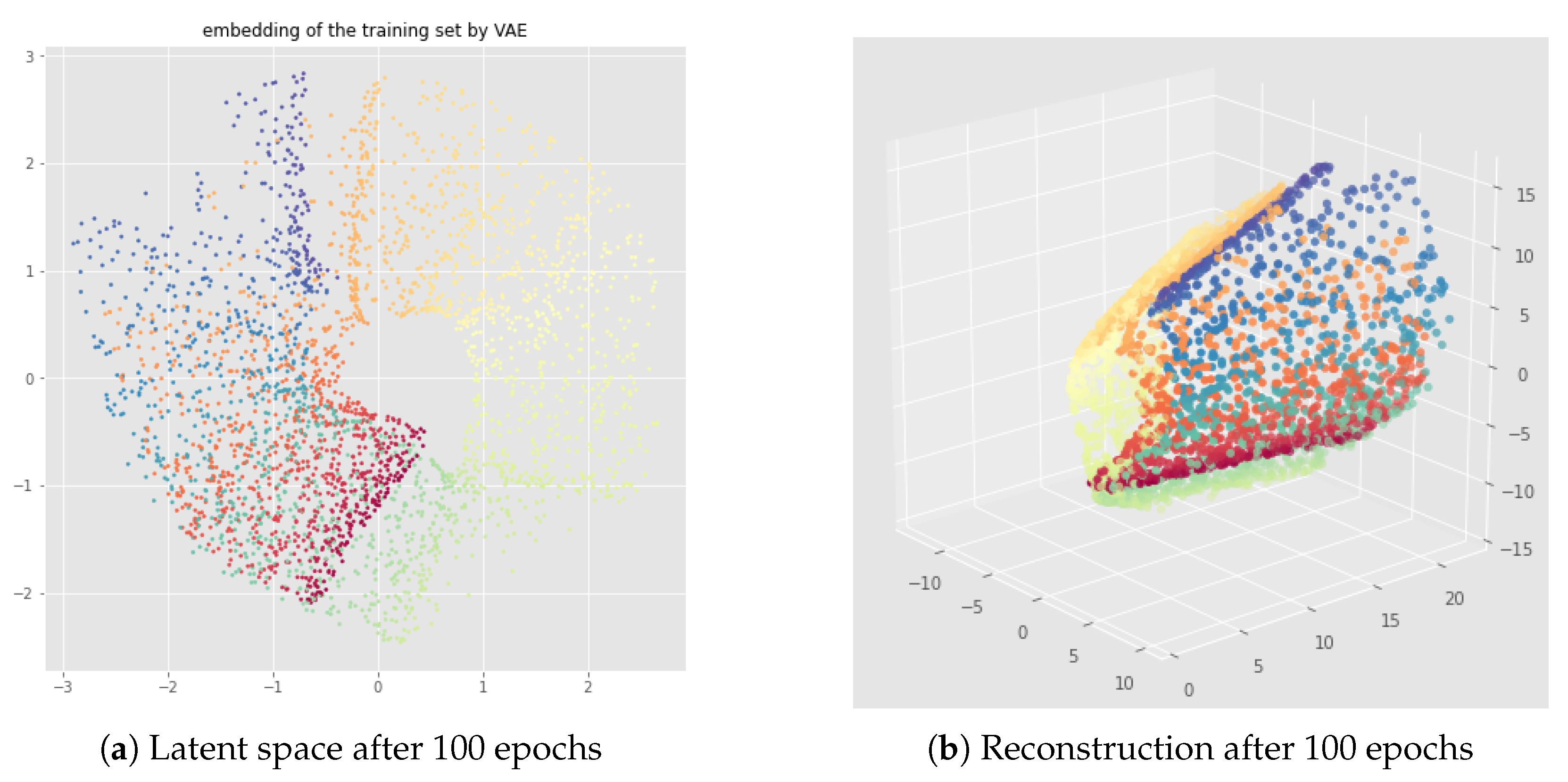
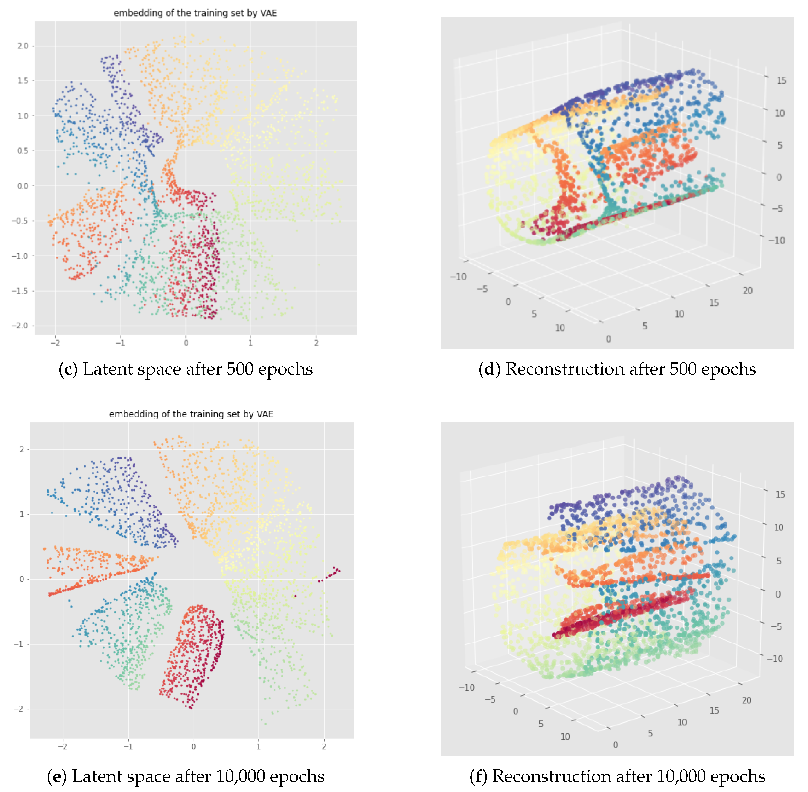
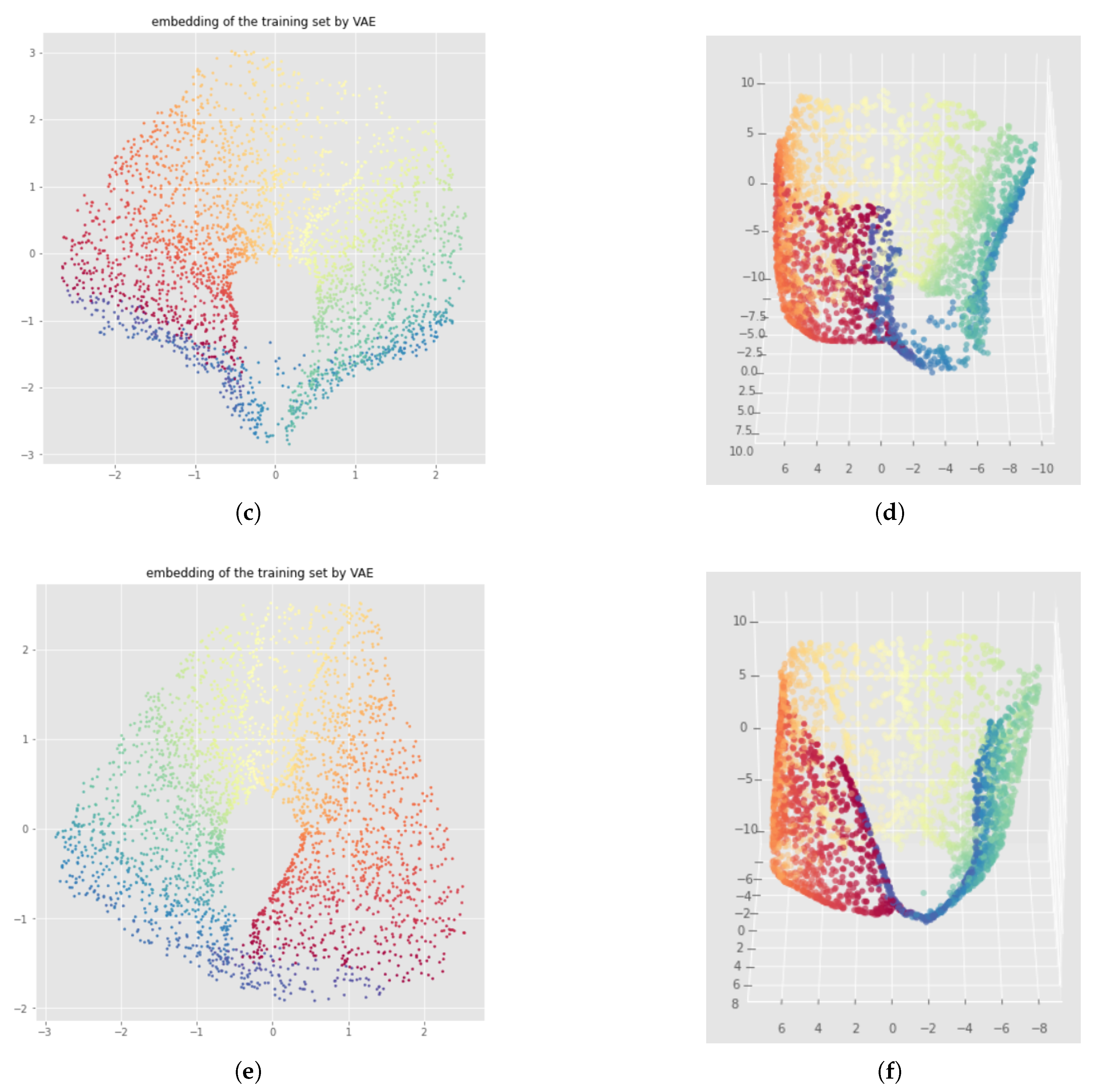
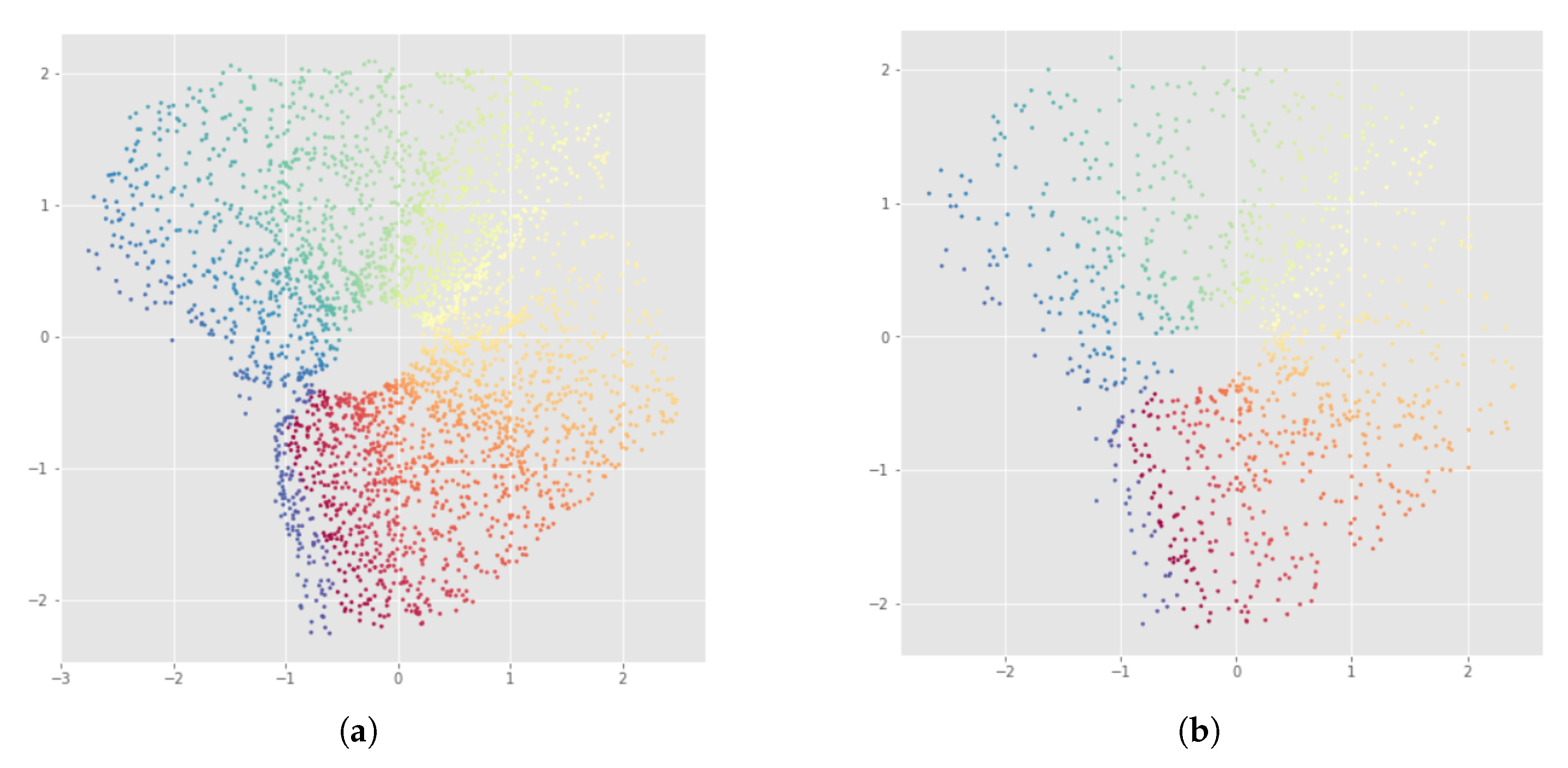
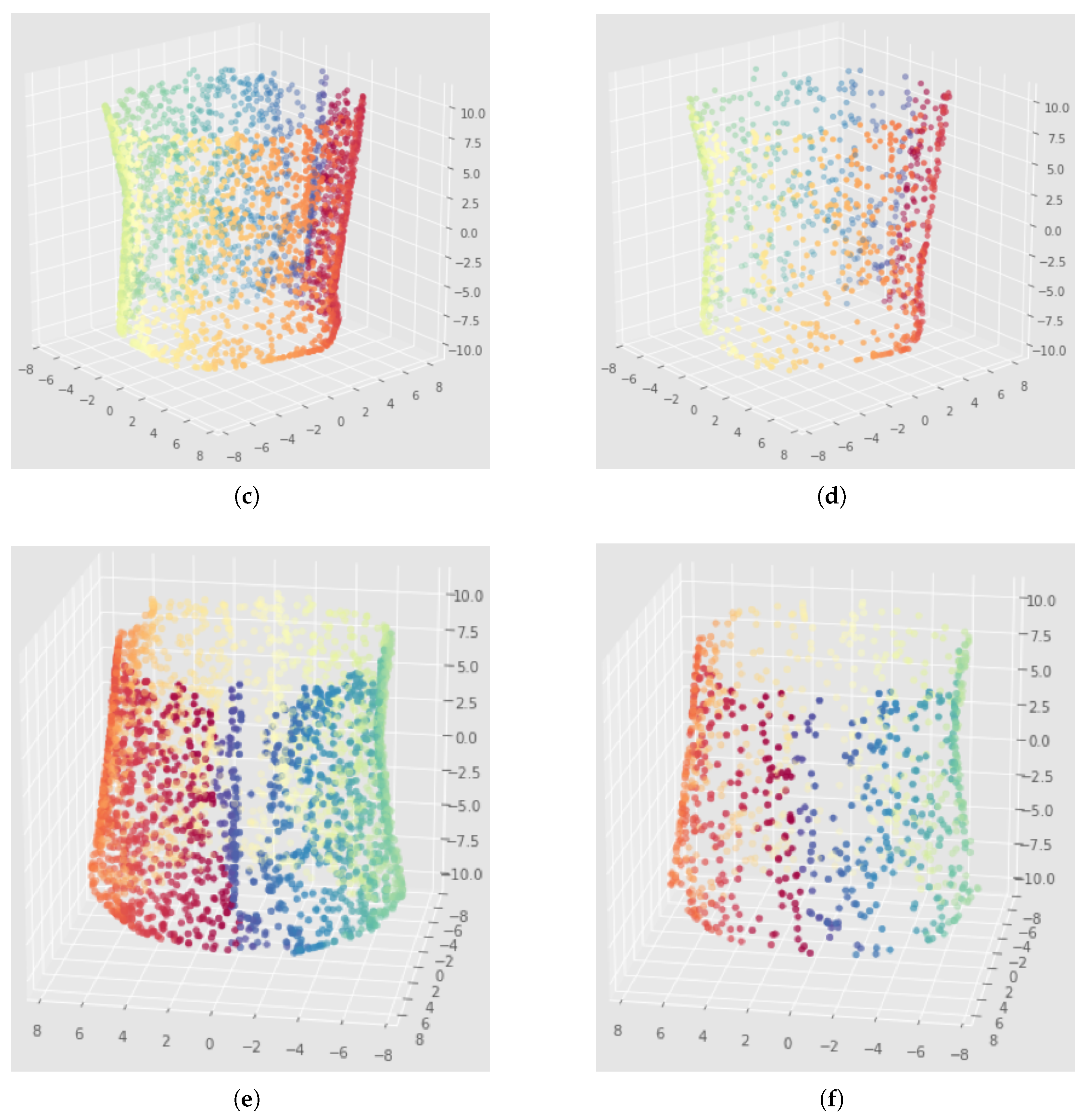
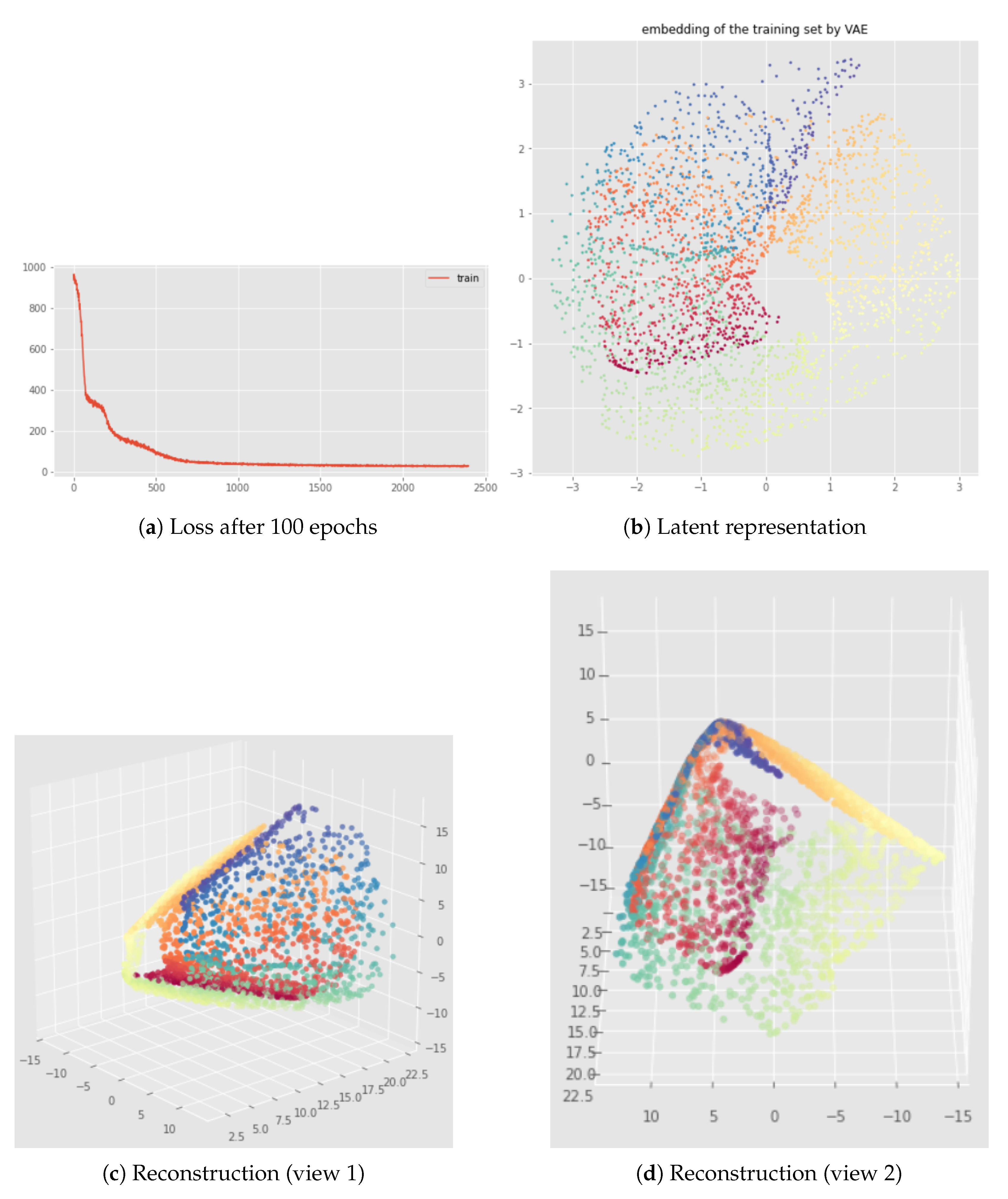
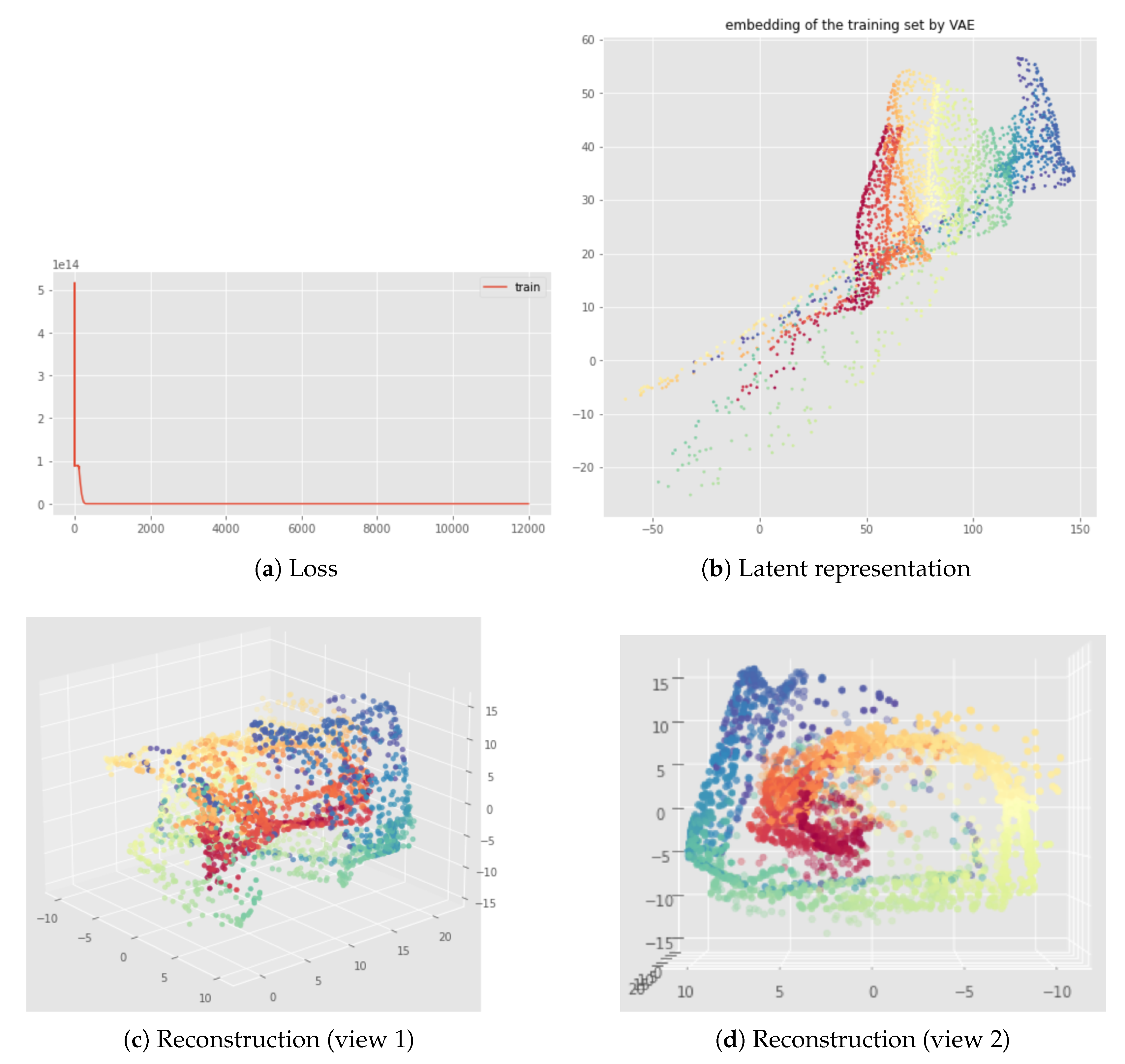
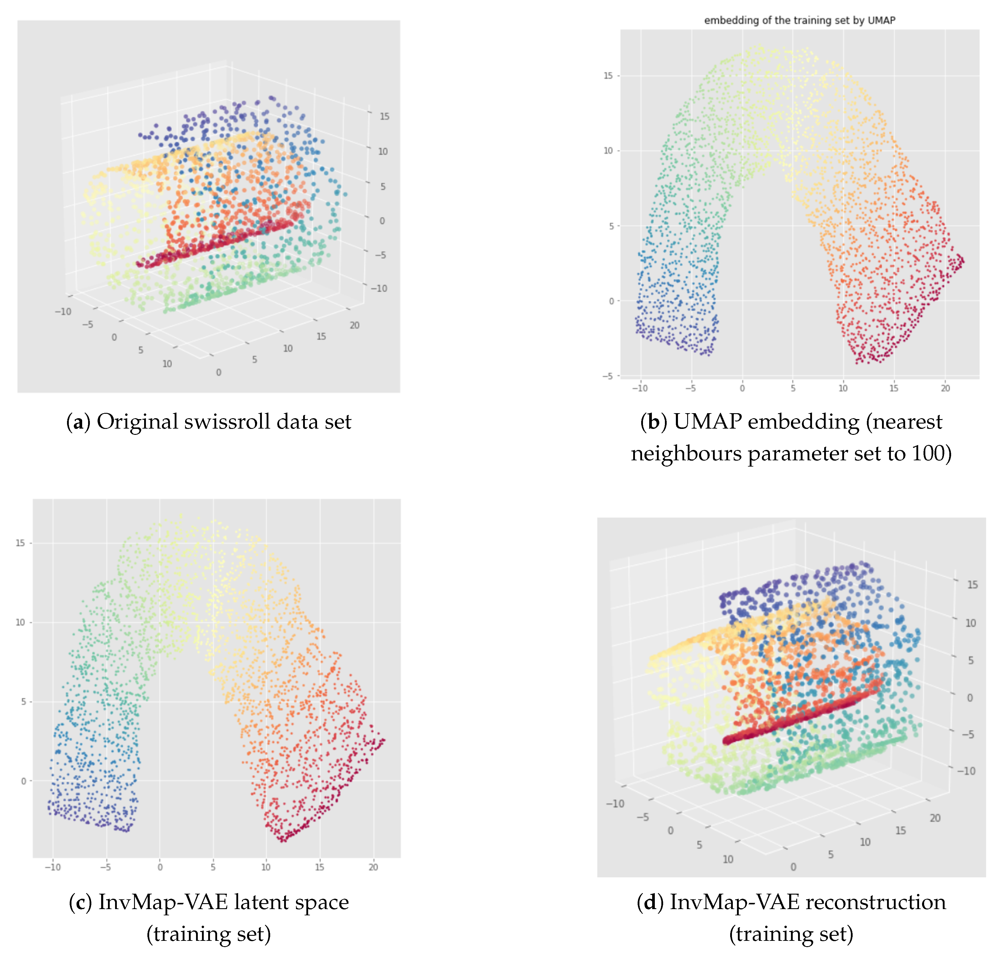
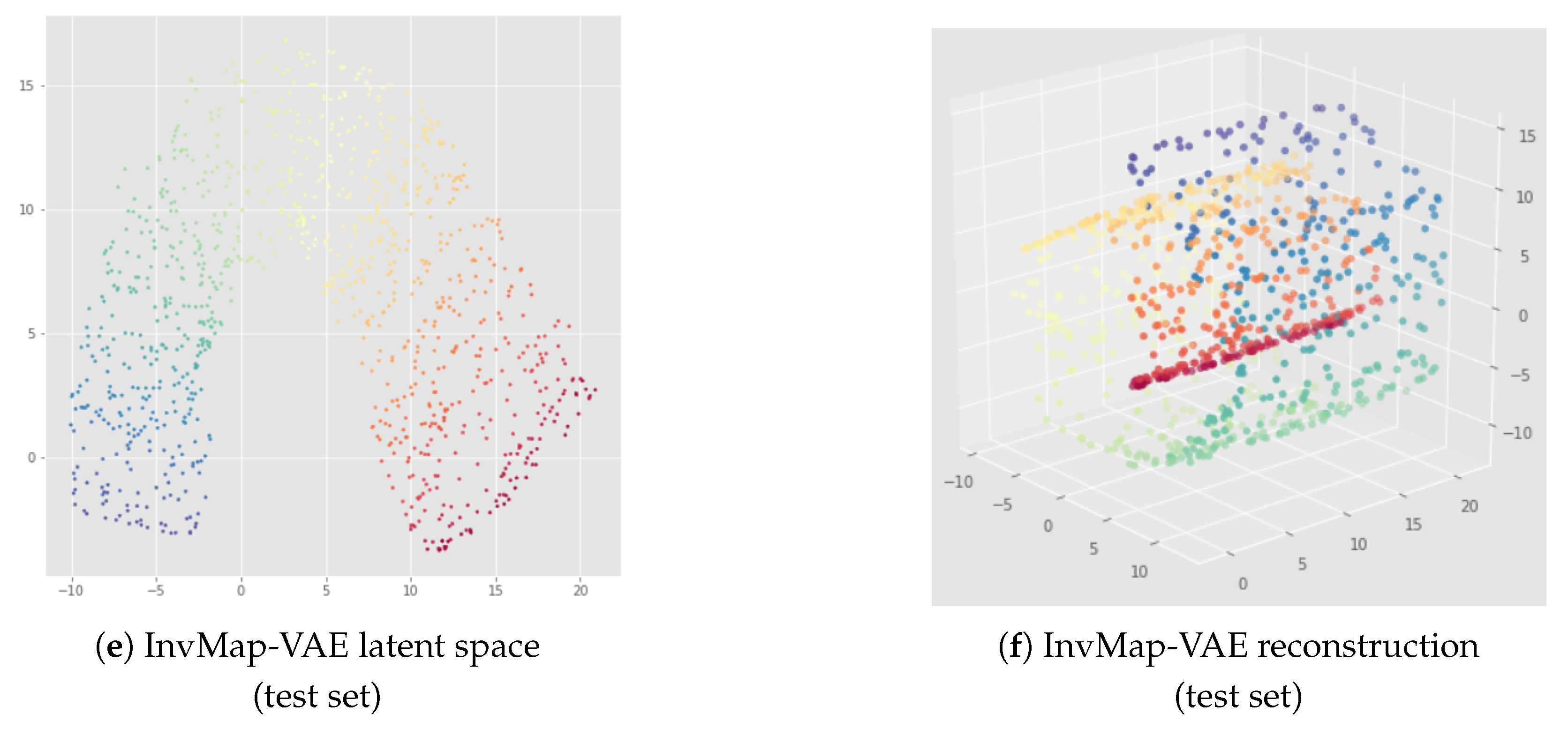
6.2. Results

The results of an Isomap-based InvMap-VAE are given in Figure 15 for the open cylinder and Figure 16 and Figure 17 for the swissroll. The neural network weights initializations does not affect these results, meaning that this method is consistent. As we can see, both for the open cylinder and for the swissroll dataset, the topology is preserved. This is because Isomap preserved the topology as we can visualize it with the Isomap embeddings. Furthermore, depending on the parameters chosen for Isomap, Isomap and thus the corresponding InvMap-VAE can either flatten the swissroll, like in Figure 16, or preserve the global spiral structure, like in Figure 17. See Appendix B for extended results with a UMAP-based InvMap-VAE where same conclusions can be drawn.

We can conclude that InvMap-VAE is consistent, and more importantly, if the given embedding preserves the topology, then the corresponding InvMap-VAE is also topology-aware. This method is a simple way to turn a dimensionality reduction technique into a generative model since the VAE framework allows one to sample from the latent space and generate new data. In the next section, we wanted to develop a topology-aware VAE that does not need any embedding as input.

7. Witness Simplicial VAE

We present in this section our second method called “Witness Simplicial VAE”. On the contrary to our previous method, this one does not depend on any other dimensionality reduction technique or embedding. It has a pre-processing step where a witness complex is built considering the topological information that should be kept. Then, comes the learning process with a VAE regularized using the constructed witness complex.

7.1. Method

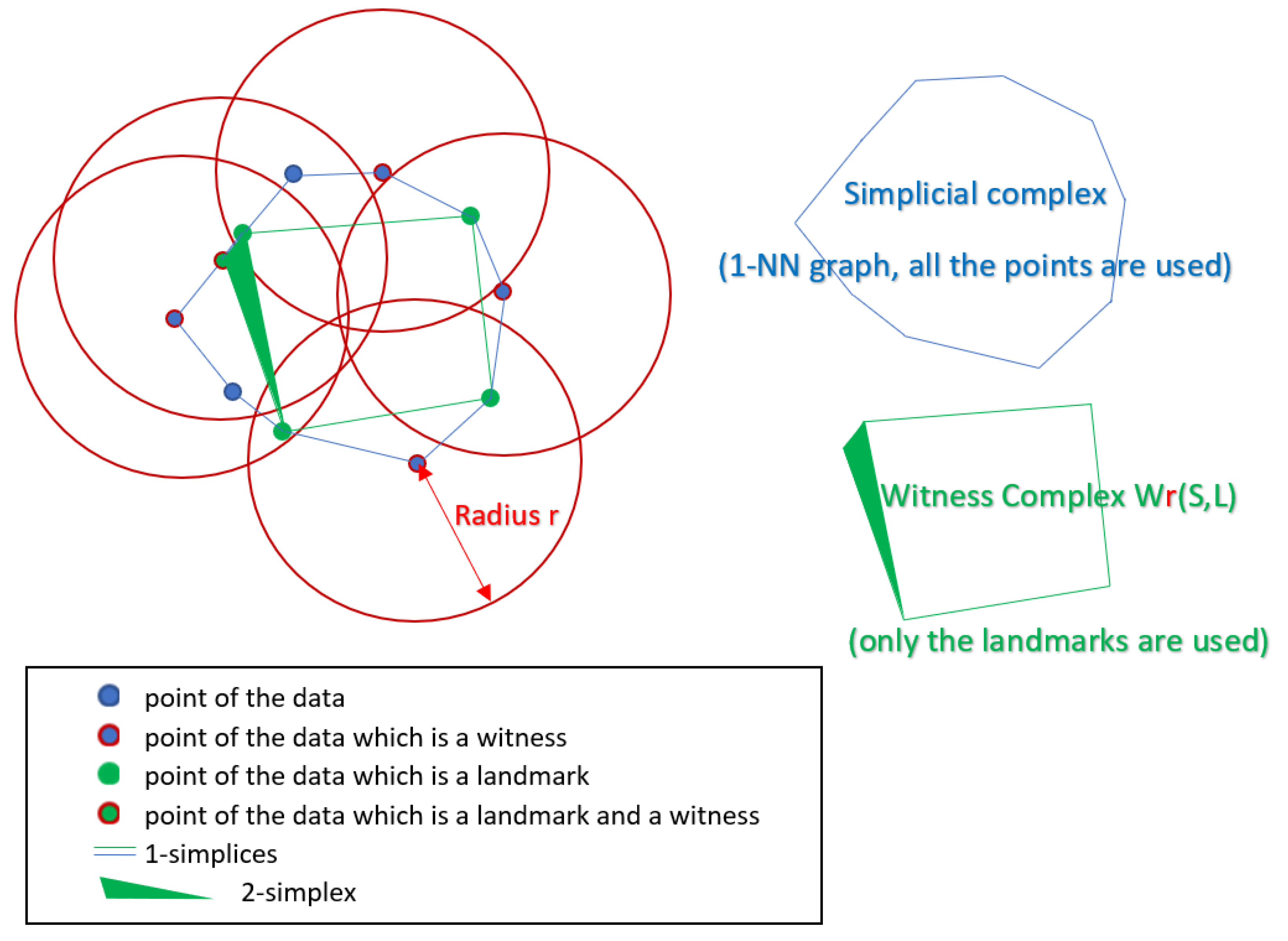
7.1.1. Witness Complex Construction

We propose here to build a witness complex in the original data space, and then try to preserve this simplicial complex structure of the data when going to the latent space of a VAE. Thus, the topology of the witness complex would be preserved. Since the witness complex allows us to do topological approximation, we should build a witness complex relevant to the topological information we want to keep. Additionally, to construct the witness complex, one should consider only the simplices of dimension lower or equal to the dimension of the latent space, which is good since computations of higher order dimensional simplices are thus avoided.

At first, we choose randomly a number of landmarks points and we define all the points of the data as witnesses. The choice of the landmarks is made randomly, as suggested in [11], also, a subset of the data could be used for the witnesses for less computations. Then, a witness complex can be built given a radius. To choose a relevant radius, we first perform a witness complex filtration to obtain a persistence diagram. After that, we choose a radius such that the Betti numbers of the witness complex constructed with this radius, are the persistent Betti numbers given by this persistence diagram. Indeed, we know from topological data analysis that the relevant topological information is given by the persistent Betti numbers.

Illustrations of this process are given in Figure 18. At first in (a), we perform a witness complex filtration choosing randomly 10 landmarks points (in practice we stopped the filtration after a high enough radius filtration). Then, we look at the persistence diagram (a) and we choose a radius relevant to the problem, that is a filtration radius such that the topological information we want to preserve is present in the witness complex. In this case, we see in (a) at $x\sim 5.9$ a blue point corresponding to Betti 1 which persists (because far from the diagonal $y=x$). This point represents the topology we want to preserve: the “cycle” structure of the open cylinder (the 1-dimensional hole). That is why in (b) we choose a witness complex built from this filtration stopping at $r_{filtration}=6$ and for which we have ${\beta }_1=1$. (c) and (d) are different views of the 1-simplices (grey edges) of this witness complex. (e) and (f) show the impact of increasing the number of landmarks: we obtain more simplices which implies more computations and possibly not relevant 1-dimensional holes. However, increasing the number of landmarks should help to obtain a topological structure more robust to noise and outliers.

See Appendix C for examples of bad witness complex constructions that should be avoided by being careful to the parameters chosen (landmarks and radius) and by visualizing it if possible.

7.1.2. Witness Complex Simplicial Regularization

Once we have a witness complex built from the original input data, we can define a simplicial regularization by adding a term to the VAE loss. The idea of a simplicial regularization combined to an auto-encoder framework was recently introduced first by Jose Gallego-Posada in his master thesis [28] as a generalization of the “mixup” regularization ([30,31]). We incorporate the simplicial regularization in a variational auto-encoder framework, however, here we use it in a different way than [28] for at least two aspects:

• It does not depend on any embedding whereas in [28] the author was relying on a UMAP embedding for his simplicial regularization of the decoder.
• We use only one witness simplical complex built from the input data whereas the author of [28] was using one fuzzy simplicial complex built from the input data and a second one built from the UMAP embedding and both were built via the fuzzy simplicial set function provided with UMAP (keeping only simplices with highest probabilities).

Below is how we define the simplicial regularizations (largely) inspired by [28], for the encoder and the decoder, using a unique simplicial complex which is here a witness complex:

$${\mathcal{L}}_{SE}(e,K,\alpha )=\sum _{\sigma \in K}{\mathbb{E}}_{{\lambda }_j\sim Dir(dim\left(\sigma \right)+1,\alpha )}\mathrm{MSE}\left(e\left(\sum _{j=0}^{dim\left(\sigma \right)}{\lambda }_j{\sigma }_j\right),\sum _{j=0}^{dim\left(\sigma \right)}{\lambda }_{j}e\left({\sigma }_j\right)\right)$$

(3)

$${\mathcal{L}}_{SD}(d,K,\alpha )=\sum _{\sigma \in K}{\mathbb{E}}_{{\lambda }_j\sim Dir(dim\left(\sigma \right)+1,\alpha )}\mathrm{MSE}\left(d\left(\sum _{j=0}^{dim\left(\sigma \right)}{\lambda }_{j}e\left({\sigma }_j\right)\right),\sum _{j=0}^{dim\left(\sigma \right)}{\lambda }_{j}d\left(e\left({\sigma }_j\right)\right)\right)$$

(4)

With:

• ${\mathcal{L}}_{SE}$ the simplicial regularization term for the encoder.
• ${\mathcal{L}}_{SD}$ the simplicial regularization term for the decoder.
• e and d, respectively, the (probabilistic) encoder and decoder.
• K a (witness) simplicial complex built from the input space.
• $\sigma$ a simplex belonging to the simplicial complex K.
• ${\sigma }_j$ the vertex number j of the $dim\left(\sigma \right)$-simplex $\sigma$ which has exactly $dim\left(\sigma \right)+1$ vertices. ${\sigma }_j$ is, thus, a data point in the input space X.
• $\mathrm{MSE}(a,b)$ the Mean Square Error between a and b.
• ${\mathbb{E}}_{{\lambda }_j\sim Dir(dim\left(\sigma \right)+1,\alpha )}$ the expectation for the ${\left({\lambda }_j\right)}_{j=0,\dots ,dim\left(\sigma \right)}$ following a symmetric Dirichlet distribution with parameters $dim\left(\sigma \right)+1$ and $\alpha$. When $\alpha =1$, which is what we used in practice, the symmetric Dirichlet distribution is equivalent to a uniform distribution over the $dim\left(\sigma \right)$-simplex $\sigma$, and as $\alpha$ tends towards 0, the distribution becomes more concentrated on the vertices.

Finally, if we note $w_{SE}$ and $w_{SD}$ the weights of the additional terms, the loss of the Witness Simplicial VAE is:

$${\mathcal{L}}_{WSVAE}={\mathcal{L}}_{VAE}+w_{SE}\times {\mathcal{L}}_{SE}+w_{SD}\times {\mathcal{L}}_{SD}$$

(5)

The motivation is actually, by minimizing ${\mathcal{L}}_{SE}$ and ${\mathcal{L}}_{SD}$ in Equation (5), to “force” both the encoder and the decoder to become (continuous) simplicial maps. Indeed, minimizing ${\mathcal{L}}_{SE}$ forces the encoder to be a simplicial map between the witness complex of the input data space and its image by the encoder, and minimizing ${\mathcal{L}}_{SD}$ forces the decoder to be a simplicial map between the latent space and the output reconstruction space. We can actually see that the MSE term both in (3) and (4) measures, respectively, “how far the encoder and the decoder are from being simplicial maps” [28]. Indeed, if they were simplicial maps then the MSE would be equal to zero by definition of a simplicial map. This should be true for any $({\lambda }_0,\dots ,{\lambda }_{dim\left(\sigma \right)})\in {\mathbb{R}}_{+}^{dim\left(\sigma \right)+1}$, such that ${\sum }_{i=0}^{dim\left(\sigma \right)}{\lambda }_i=1$ with $\sigma$ being any simplex of K. In practice, we do a Monte Carlo estimation, that is we sample a certain number of times (denoted $N_{LambdasSamples}$) the lambdas from a uniform distribution (i.e., a Dirichlet distribution with parameter $\alpha =1$) over the simplex $\sigma$ and we take the expectation. Given a simplex $\sigma \in K$, sampling the lambdas coefficients $({\lambda }_0,\dots ,{\lambda }_{dim\left(\sigma \right)})$ is equivalent to sample a point in the convex hull spanned by the vertices of $\sigma$. Thus, minimizing ${\mathcal{L}}_{SE}$ is equivalent to do data augmentation and “forcing” the image of this point by the encoder to be in the convex hull spanned by the images of the vertices of $\sigma$ by the encoder and with the same lambdas coefficients. So this “forces” the encoder to be a linear map on the simplices of K, exactly like a simplicial map. The same reasoning can be applied to the decoder when minimizing ${\mathcal{L}}_{SD}$.

In addition to that, we know from algebraic topology that a simplicial map induces well-defined homomorphisms between the homology groups (for details see lemma 6.2 page 65 of the Section 6 on “Simplicial Homology Groups” of the course [10]). Furthermore, minimizing ${\mathcal{L}}_{VAE}$ in Equation (5) implies to minimize the reconstruction error which allows one to obtain injective encoder and decoder, if we neglect their probabilistic aspect (for example by considering the means instead of the probability distributions). Thus, this should give a bijective simplicial map. So, finally, the encoder (and decoder) would induce isomorphisms between the homology groups given the simplicial complex, implying that the Betti numbers, and, thus, the persistent Betti numbers, between the latent representation and the witness complex built from the input data would be the same when the loss ${\mathcal{L}}_{WSVAE}$ is converging.

To conclude, this should make the Witness Simplicial VAE topology-aware by preserving relevant topological information (i.e., the persistent Betti numbers) between the input data and its latent representation.

7.1.3. Witness Simplicial VAE

We can summarize the method of the Witness Simplicial VAE as follows:

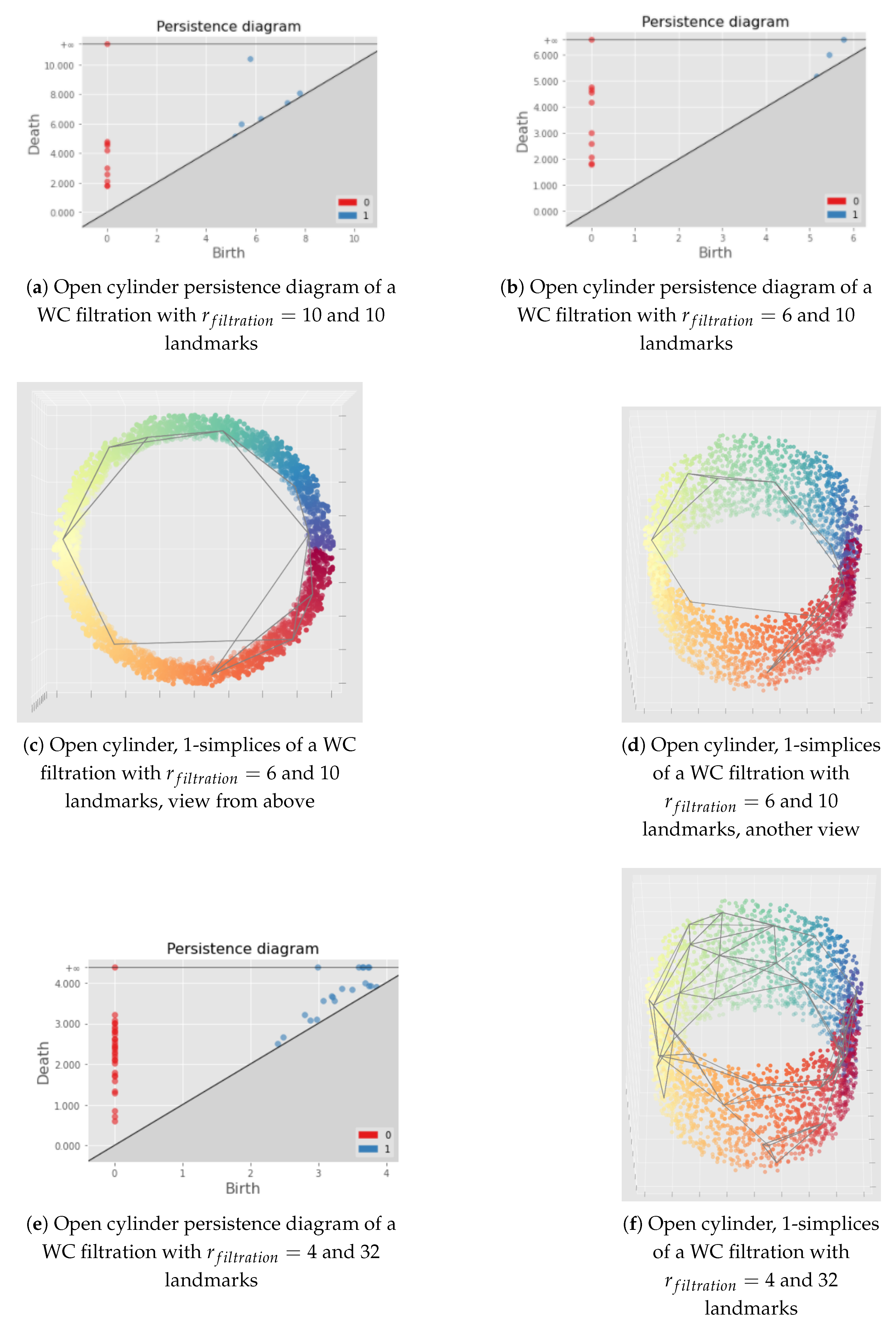
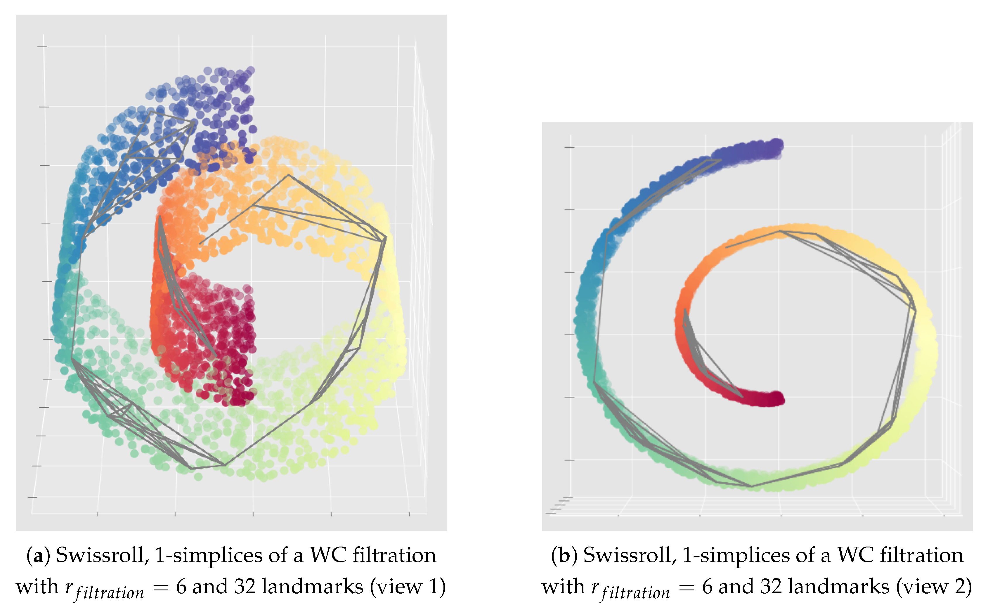
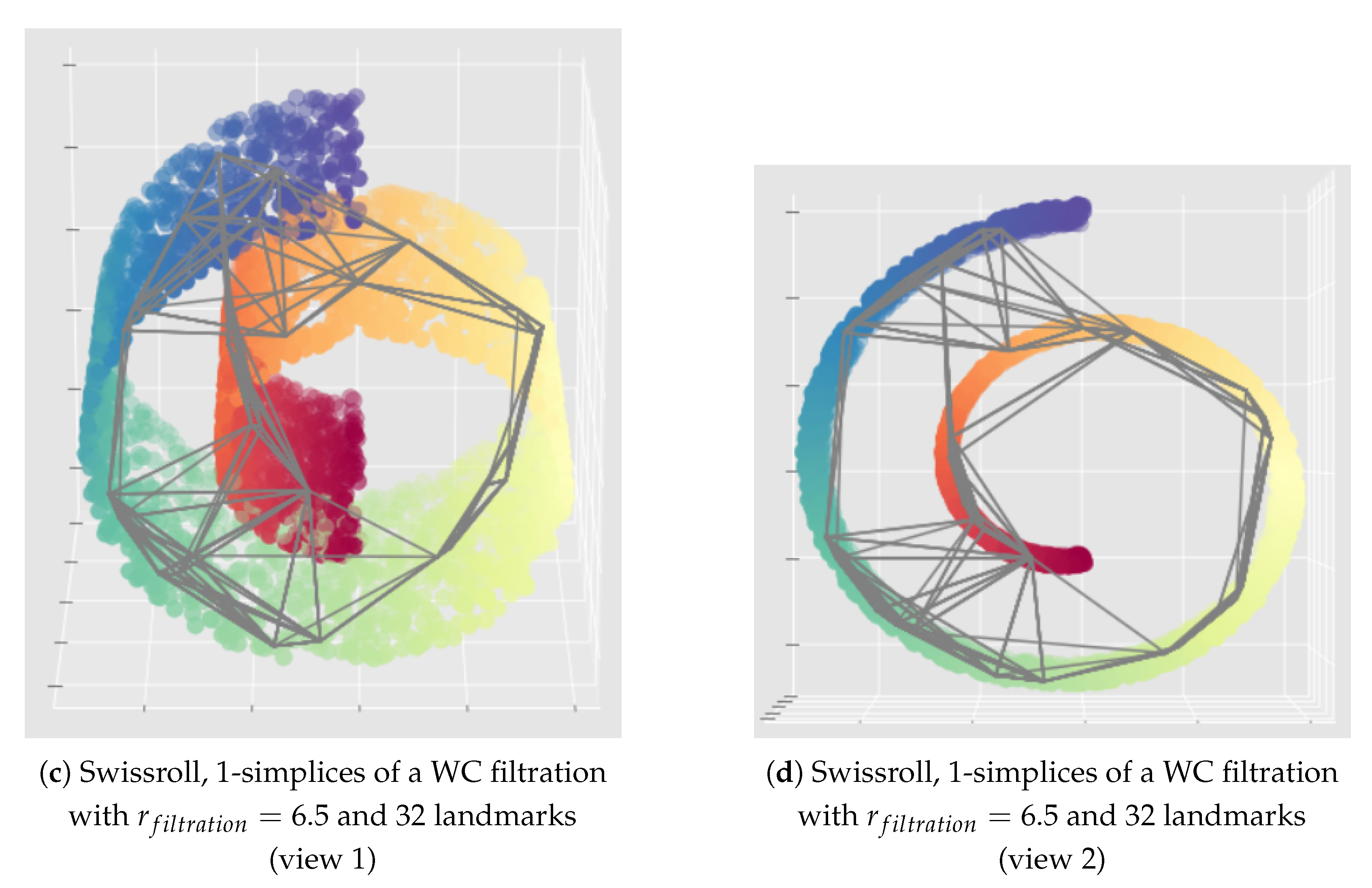
• Perform a witness complex filtration of the input data to obtain a persistence diagram (or a barcode).
• Build a witness complex given the persistence diagram (or the barcode) of this filtration, and potentially any additional information on the Betti numbers which should be preserved according to the problem (number of connected components, 1-dimensional holes…).
• Train the model using this witness complex to compute the loss ${\mathcal{L}}_{WSVAE}$ of Equation (5).

Steps one and two are pre-processing steps to compute the witness complex, then this same witness complex is used during the whole training process for the learning part which is step three.

For the step one we need to choose the landmarks points. The more landmarks we have the more the witness complex will capture the topology of data, but the more the model will be computationally expensive because of a high number of simplices to consider in the summations over simplices when computing the simplicial regularizations. So this choice is a trade-off between “topological precision” and computational complexity.

Then, for the step two comes the choice of the filtration radius $r_{filtration}$, this depends on the problem and which Betti numbers are important to preserve. We assume that the latter are actually the persistent Betti numbers. In our experiments we focused on preserving 0-homology and 1-homology since our latent space is 2-dimensional, but the method is not limited to that: any dimensional topological features could in theory be preserved.

Lastly, the step three is performed through stochastic gradient descent as for the standard VAE. The correct weights $w_{SE}$ and $w_{SD}$ should be found by grid search, in our experiments we kept $w_{SE}=w_{SD}$ for less possible combinations. The number of samples $N_{LambdasSamples}$ for the estimation of the expectation with the Dirichlet distribution needs also to be chosen, we assumed that $N_{LambdasSamples}=10$ should be enough. The choice of $N_{LambdasSamples}$ is also a trade-off between the performance and the computational complexity. Additionally, if the number of simplices in the witness complex is too high and cannot be reduced, then for less computations one can consider only a subset of the simplices at each batch instead of considering them all, but making sure that (almost) all the subsets are considered within one epoch.

Finally, we can highlight that we chose to use a Witness complex for its computational efficiency, compared to other usual simplicial complexes, such as the Čech or Vietoris–Rips complexes. These ones could also be used in theory but would have too many simplices to process in practice for computing the simplicial regularizations whereas the witness complex has less simplices as it provides a topological approximation.

7.1.4. Isolandmarks Witness Simplicial VAE

Given the results presented in the next section, we developed an extension of the Witness Simplicial VAE to obtain better latent representations. It consists of adding another term to the loss in order to preserve some distances. Since the witness complex is constructed such that the landmarks points and their edges incorporate the relevant topology, it makes sense to add a term in order to preserve the pairwise approximate geodesic distances between the landmarks points only, instead of considering all the points of the dataset to avoid too many computations. We were inspired by the Isomap algorithm [16] and called this new approach “Isolandmarks Witness Simplicial VAE”. It can be seen as a Witness Simplicial VAE, combined with Isomap applied to the landmarks points considered in the 1-skeleton of the witness complex. More precisely, it consists of the following additional pre-processing step after having constructed the witness complex: compute the approximate geodesic distances between any two landmarks points using the graph of the witness complex (the 1-skeleton) by summing the edges euclidean distances of the shortest path between these two points. Then, we add to the loss of the Witness Simplicial VAE a term to minimize the distance between this approximate geodesic distance matrix of the landmarks points (i.e., in the input space), and the Euclidean distance matrix of the encodings of the landmarks points (i.e., in the latent space).

Finally, if we note $w_{iso}$ the weight of the additional term, the loss of Isolandmarks Witness Simplicial VAE can be written as:

$${\mathcal{L}}_{IWSVAE}={\mathcal{L}}_{WSVAE}+w_{iso}\times \frac{\parallel K\left(D^{*}\right)-K\left(D\right){\parallel }_F}{l}$$

(6)

With:

• ${\mathcal{L}}_{WSVAE}$ the loss of the Witness Simplicial VAE.
• l the number of landmarks.
• ${\parallel .\parallel }_F$ the Frobenius norm.
• $D^{*}$ the approximate geodesic distance matrix of the landmarks points in the input space computed once before learning.
• D the Euclidean distance matrix of the encodings of the landmarks points computed at each batch.
• K the Isomap kernel defined as $K\left(D\right)=-0.5(I-\frac{1}{l}A)D^2(I-\frac{1}{l}A)$ with I the identity matrix and A the matrix composed only by ones.

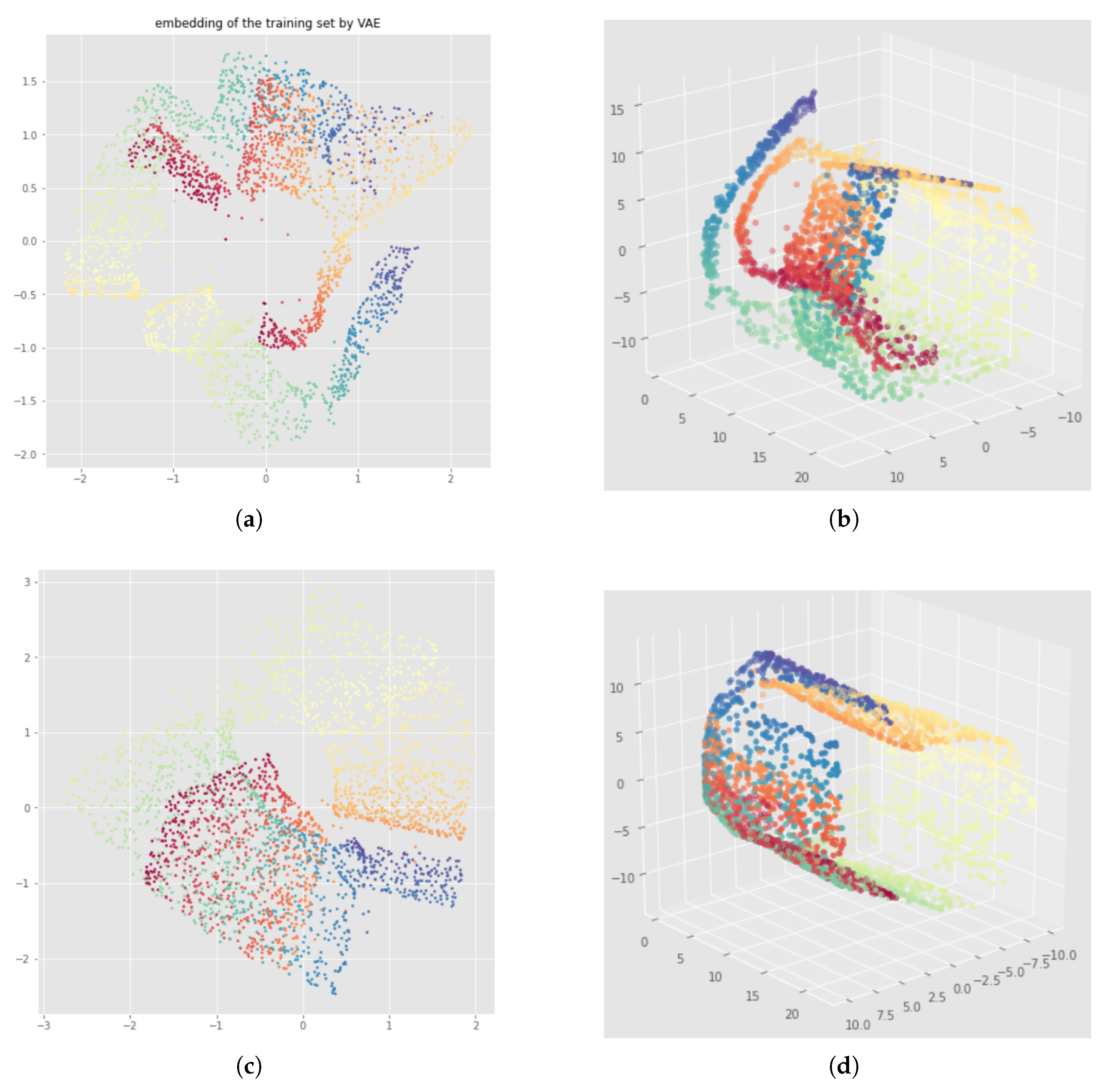
7.2. Results

This method is quite consistent when changing the neural network weights initialization as we can see in Figure 19, which shows the results for a model applied to the open cylinder dataset trained for only 100 epochs. We can see that the Betti numbers are preserved (one connected component and one 1-dimensional hole). However there are some discontinuities in the latent representation so the whole topology is not preserved. The impact of this discontinuity on the reconstruction is much less important when the model is trained more like in the Figure 20 (see the blue region). This figure is a representative result given by a Witness Simplicial VAE trained on 1000 epochs. We can see that the results are similar between the training set and the unseen test set.

However, in rare cases with the same hyperparameters than Figure 19 and Figure 20, we can obtain much less satisfactory results for some other neural network weights initialization as exposed in Appendix D. Although the latent representation and the reconstruction can have discontinuities, the persistent Betti numbers are still preserved (${\beta }_0=1$ and ${\beta }_1=1$).

For the swissroll dataset, the Witness Simplicial VAE with the hyperparameters we have tried fails to preserve the persistent Betti numbers. The best results are similar and look like the ones in Figure 21 which are not satisfactory: the latent representation has ${\beta }_0=1$ as expected but ${\beta }_1=1$ instead of 0. Indeed, because of an overlapping between the beginning and the end of the swissroll, we can see that a 1-dimensional hole appeared in the latent representation although the input data does not have that. The reconstruction is bad but this can be explained by the small number of epochs used here. However, we can say again that the method is also consistent with the swissroll dataset since the results are not really affected when changing only the neural network weights initialization. Furthermore, the results are very similar to the best we can obtain with a standard VAE (like in Figure 13).

Regarding the overlapping problem encountered with the swissroll dataset, we can see in Figure 22 that Isolandmarks Witness Simplicial VAE manages to solve it. Indeed, geometric information can help for retrieving the correct topology and with this approach the previously encountered overlapping in the latent representation of the swissroll is better avoided although the reconstruction is not perfect.

Finally, the main conclusion from these results is that with the Witness Simplicial VAE, the persistent Betti numbers, between the input and the latent space, do not decrease although they can increase. In other words, the holes in the input space are recovered in the latent space, but new holes can appear in the latent space although they were not existing in the input space. However, the extended version, that is Isolandmarks Witness Simplicial VAE, manages to preserve the persistent Betti numbers for the dataset considered.

8. Discussion

As we have seen, our first method “InvMap-VAE” is quite simple and works very well, but relies on a given embedding. This dependence might be problematic for example if this embedding comes from a dimensionality reduction technique that is not scalable or not topology-aware with more complex datasets. Additionally, it is data-dependent, that is InvMap-VAE trained with the embedding of a particular dataset might not give a meaningful latent representation when applied to another dataset, although it worked well on unseen test data points sampled from the same distribution than the training set. Thus, for a new dataset coming from a different manifold, the embedding of the new dataset might need to be given in order to learn the corresponding InvMap-VAE.

On the other side, our second method “Witness Simplicial VAE” is designed to be a topology-aware VAE independent of any other dimensionality reduction method or any embedding. On the contrary to the Topological AE [26], a limitation of our method is that it does not necessarily allow us to preserve multi-scale topological features, but it aims to preserve the topological features across multiple homology dimensions of a chosen scale corresponding to the choice of the filtration radius. It is interesting in a theoretical point of view since our method is justified with tools from computational topology that are not commonly used in the machine learning community. However, the work is still in progress since the experimental results are not completely satisfying, in particular for the swissroll dataset that is not well unrolled in the latent representation. A difficulty with this method is to find the right hyper parameters: the number of landmarks and how to choose them, the filtration radius to build a relevant witness complex, the number of samples $N_{LambdasSamples}$ for the Monte Carlo estimation of the expectation with the Dirichlet distribution to compute the simplicial regularizations, and the weights $w_{SE}$ and $w_{SD}$ of the latter in the loss. The model can be quite sensitive to these hyper parameters and lead to different latent representations. However, once these hyper parameters are fixed, the model is quite stable to the initialization of the neural network weights on the contrary to the standard VAE. Regarding the choice of the landmarks points, we made it uniformly random among the data points, but if the data density is highly heterogeneous then this could be problematic. In such case we might end up with no landmarks points in low-density regions and the topology would not be well captured by the witness complex. That is why a better way of choosing the landmarks points could be investigated. The more landmarks points are used, the more the topology can be captured and preserved, but the more it is computationally expensive.

9. Conclusions

This paper has presented two different approaches to make variational auto-encoders topology-aware: InvMap-VAE and Witness Simplicial VAE.

InvMap-VAE is a VAE with a similar latent representation to a given embedding, the latter can come from any dimensionality reduction technique. This means that if the topology is preserved in the given embedding, then InvMap-VAE is also topology-aware. Indeed, we successfully managed to preserve the topology with a Isomap-based InvMap-VAE for two different manifolds which were the open cylinder and the swissroll datasets. Moreover, the learned encoder of InvMap-VAE allows one to map a new data point to the embedding, and the learned decoder provides an inverse mapping. Thus, it allows one to turn the dimensionality reduction technique into a generative model from which new data can be sampled. An interesting future work direction would be to apply this method to real world datasets and incorporate the «parametric» Riemannian metric developed by Arvanitidis in [41] into InvMap-VAE in order to perform interpolations in the latent space. This would be a way to learn a Riemannian metric, using the «pull-back metric» of the decoder, and compute the geodesics in a latent space that is similar to the embedding given by any dimensionality reduction technique.

Witness Simplicial VAE is a VAE with a simplicial regularization computed using a witness complex built from the input data space. This second method does not depend on any embedding, and is designed such that relevant topological features called persistent Betti numbers should be preserved between the input and the latent spaces. We justified the theoretical foundations of this method using tools from algebraic topology, and noticed that it preserved the persistent Betti numbers for one manifold but not for the other one. For the open cylinder dataset, the persistent Betti numbers were indeed preserved, but we could notice that this was not enough to preserve the continuity. However, even in the failure case with the swissroll dataset, the results were consistent and not as dependent as the standard VAE on the initialization of the neural network weights, providing some stability. Finally, with Isolandmarks Witness Simplicial VAE we proposed an extension of this method that allows to better preserve the persistent Betti numbers with the swissroll dataset. We leveraged the topological approximation given by the witness complex to preserve some relevant distances, that is the pairwise approximate geodesic distances of the landmarks points between the input and the latent spaces. Future work could be to try a simplicial regularization computed through other kind of simplicial complexes, for example with a k-nearest-neighbours witness complex as used in [42].

Finally, other future work directions could be to investigate if such topology-aware VAEs are more robust against adversarial attacks as suggested in [43].

References

- Goodfellow, I.; Pouget-Abadie, J.; Mirza, M.; Xu, B.; Warde-Farley, D.; Ozair, S.; Courville, A.; Bengio, Y. Generative Adversarial Nets. In Advances in Neural Information Processing Systems 27 (NIPS 2014); Ghahramani, Z., Welling, M., Cortes, C., Lawrence, N., Weinberger, K.Q., Eds.; Curran Associates, Inc.: Red Hook, NY, USA, 2014; Volume 27. [Google Scholar]
- Kingma, D.P.; Welling, M. Auto-Encoding Variational Bayes. In Proceedings of the ICLR, Banff, AB, Canada, 14–16 April 2014. [Google Scholar]
- Rezende, D.J.; Mohamed, S.; Wierstra, D. Stochastic Backpropagation and Approximate Inference in Deep Generative Models. In Proceedings of the 31st International Conference on Machine Learning, Beijing, China, 21–26 June 2014; Xing, E.P., Jebara, T., Eds.; PMLR: Bejing, China, 2014; Volume 32, pp. 1278–1286. [Google Scholar]
- Medbouhi, A.A. Towards Topology-Aware Variational Auto-Encoders: From InvMap-VAE to Witness Simplicial VAE. Master’s Thesis, KTH Royal Institute of Technology, Stockholm, Sweden, 2022. [Google Scholar]
- Hensel, F.; Moor, M.; Rieck, B. A Survey of Topological Machine Learning Methods. Front. Artif. Intell. 2021, 4, 52. [Google Scholar] [CrossRef] [PubMed]
- Ferri, M. Why Topology for Machine Learning and Knowledge Extraction? Mach. Learn. Knowl. Extr. 2019, 1, 115–120. [Google Scholar] [CrossRef]
- Edelsbrunner, H.; Harer, J. Computational Topology-an Introduction; American Mathematical Society: Providence, RI, USA, 2010; pp. I–XII, 1–241. [Google Scholar]
- Wikipedia, the Free Encyclopedia. Simplicial Complex Example. 2009. Available online: https://en.wikipedia.org/wiki/File:Simplicial_complex_example.svg (accessed on 18 March 2021).
- Wikipedia, the Free Encyclopedia. Simplicial Complex Nonexample. 2007. Available online: https://commons.wikimedia.org/wiki/File:Simplicial_complex_nonexample.png (accessed on 18 March 2021).
- Wilkins, D.R. Algebraic Topology, Course 421; Trinity College: Dublin, Ireland, 2008. [Google Scholar]
- de Silva, V.; Carlsson, G. Topological estimation using witness complexes. IEEE Symp. Point-Based Graph. 2004, 4, 157–166. [Google Scholar]
- Rieck, B. Topological Data Analysis for Machine Learning, Lectures; European Conference on Machine Learning and Principles and Practice of Knowledge Discovery in Databases. 2020. Available online: https://bastian.rieck.me/outreach/ecml_pkdd_2020/ (accessed on 12 November 2020).
- Pearson, K. LIII. On lines and planes of closest fit to systems of points in space. Lond. Edinb. Dublin Philos. Mag. J. Sci. 1901, 2, 559–572. [Google Scholar] [CrossRef]
- Hotelling, H. Relations Between Two Sets of Variates. Biometrika 1936, 28, 321–377. [Google Scholar] [CrossRef]
- Lee, J.A.; Verleysen, M. Nonlinear Dimensionality Reduction, 1st ed.; Springer Publishing Company, Incorporated: New York, NY, USA, 2007. [Google Scholar]
- Tenenbaum, J.B.; de Silva, V.; Langford, J.C. A Global Geometric Framework for Nonlinear Dimensionality Reduction. Science 2000, 290, 2319. [Google Scholar] [CrossRef] [PubMed]
- Kruskal, J. Multidimensional scaling by optimizing goodness of fit to a nonmetric hypothesis. Psychometrika 1964, 29, 1–27. [Google Scholar] [CrossRef]
- Kruskal, J. Nonmetric multidimensional scaling: A numerical method. Psychometrika 1964, 29, 115–129. [Google Scholar] [CrossRef]
- Borg, I.; Groenen, P. Modern Multidimensional Scaling: Theory and Applications; Springer Series in Statistics; Springer: Berlin/Heidelberg, Germany, 2005. [Google Scholar] [CrossRef]
- Van der Maaten, L.; Hinton, G. Visualizing data using t-SNE. J. Mach. Learn. Res. 2008, 9, 2579–2605. [Google Scholar]
- Hinton, G.E.; Roweis, S. Stochastic Neighbor Embedding. In Advances in Neural Information Processing Systems 15 (NIPS 2002); Becker, S., Thrun, S., Obermayer, K., Eds.; MIT Press: Cambridge, MA, USA, 2002; Volume 15. [Google Scholar]
- McInnes, L.; Healy, J.; Melville, J. UMAP: Uniform Manifold Approximation and Projection for Dimension Reduction. arXiv 2018, arXiv:1802.03426. [Google Scholar]
- Kingma, D.P.; Welling, M. An Introduction to Variational Autoencoders. Found. Trends Mach. Learn. 2019, 12, 307–392. [Google Scholar] [CrossRef]
- Gabrielsson, R.B.; Nelson, B.J.; Dwaraknath, A.; Skraba, P.; Guibas, L.J.; Carlsson, G.E. A Topology Layer for Machine Learning. arXiv 2019, arXiv:1905.12200. [Google Scholar]
- Polianskii, V. An Investigation of Neural Network Structure with Topological Data Analysis. Master’s Thesis, KTH Royal Institute of Technology, Stockholm, Sweden, 2018. [Google Scholar]
- Moor, M.; Horn, M.; Rieck, B.; Borgwardt, K.M. Topological Autoencoders. arXiv 2019, arXiv:1906.00722. [Google Scholar]
- Hofer, C.D.; Kwitt, R.; Dixit, M.; Niethammer, M. Connectivity-Optimized Representation Learning via Persistent Homology. arXiv 2019, arXiv:1906.09003. [Google Scholar]
- Gallego-Posada, J. Simplicial AutoEncoders: A connection between Algebraic Topology and Probabilistic Modelling. Master’s Thesis, University of Amsterdam, Amsterdam, The Netherlands, 2018. [Google Scholar]
- Gallego-Posada, J.; Forré, P. Simplicial Regularization. In Proceedings of the ICLR 2021 Workshop on Geometrical and Topological Representation Learning, Virtual, 3–7 May 2021. [Google Scholar]
- Zhang, H.; Cisse, M.; Dauphin, Y.N.; Lopez-Paz, D. mixup: Beyond Empirical Risk Minimization. In Proceedings of the International Conference on Learning Representations, Vancouver, BC, Canada, 30 April–3 May 2018. [Google Scholar]
- Verma, V.; Lamb, A.; Beckham, C.; Courville, A.C.; Mitliagkas, I.; Bengio, Y. Manifold Mixup: Encouraging Meaningful On-Manifold Interpolation as a Regularizer. arXiv 2018, arXiv:1806.05236. [Google Scholar]
- Khrulkov, V.; Oseledets, I.V. Geometry Score: A Method For Comparing Generative Adversarial Networks. arXiv 2018, arXiv:1802.02664. [Google Scholar]
- Perez Rey, L.A.; Menkovski, V.; Portegies, J. Diffusion Variational Autoencoders. In Proceedings of the Twenty-Ninth International Joint Conference on Artificial Intelligence, IJCAI-20, Yokohama, Japan, 11–17 July 2020; pp. 2704–2710. [Google Scholar] [CrossRef]
- Paszke, A.; Gross, S.; Massa, F.; Lerer, A.; Bradbury, J.; Chanan, G.; Killeen, T.; Lin, Z.; Gimelshein, N.; Antiga, L.; et al. PyTorch: An Imperative Style, High-Performance Deep Learning Library. In Advances in Neural Information Processing Systems 32; Wallach, H., Larochelle, H., Beygelzimer, A., d’Alché-Buc, F., Fox, E., Garnett, R., Eds.; Curran Associates, Inc.: Red Hook, NY, USA, 2019; pp. 8024–8035. [Google Scholar]
- Kingma, D.P.; Ba, J. Adam: A Method for Stochastic Optimization. arXiv 2014, arXiv:1412.6980. [Google Scholar]
- Simon, S. Witness Complex. 2020. Available online: https://github.com/MrBellamonte/WitnessComplex (accessed on 20 December 2022).
- Maria, C.; Boissonnat, J.D.; Glisse, M.; Yvinec, M. The Gudhi Library: Simplicial Complexes and Persistent Homology; Technical Report; Springer: Berlin/Heidelberg, Germany, 2014. [Google Scholar]
- Maria, C. Filtered Complexes. In GUDHI User and Reference Manual, 3.4.1th ed.; GUDHI Editorial Board: San Francisco, CA, USA, 2021. [Google Scholar]
- Pedregosa, F.; Varoquaux, G.; Gramfort, A.; Michel, V.; Thirion, B.; Grisel, O.; Blondel, M.; Prettenhofer, P.; Weiss, R.; Dubourg, V.; et al. Scikit-learn: Machine Learning in Python. J. Mach. Learn. Res. 2011, 12, 2825–2830. [Google Scholar]
- Marsland, S. Machine Learning-An Algorithmic Perspective; Chapman and Hall/CRC Machine Learning and Pattern Recognition Series; CRC Press: Boca Raton, FL, USA, 2009; pp. I–XVI, 1–390. [Google Scholar]
- Arvanitidis, G.; Hansen, L.K.; Hauberg, S. Latent Space Oddity: On the Curvature of Deep Generative Models. In Proceedings of the ICLR (Poster), Vancouver, BC, Canada, 30 April–3 May 2018. [Google Scholar]
- Schönenberger, S.T.; Varava, A.; Polianskii, V.; Chung, J.J.; Kragic, D.; Siegwart, R. Witness Autoencoder: Shaping the Latent Space with Witness Complexes. In Proceedings of the NeurIPS 2020 Workshop on Topological Data Analysis and Beyond, Virtual, 6–12 December 2020. [Google Scholar]
- Jang, U.; Jha, S.; Jha, S. On the Need for Topology-Aware Generative Models for Manifold-Based Defenses. In Proceedings of the International Conference on Learning Representations, Addis Ababa, Ethiopia, 26–30 April 2020. [Google Scholar]
Disclaimer/Publisher’s Note: The statements, opinions and data contained in all publications are solely those of the individual author(s) and contributor(s) and not of MDPI and/or the editor(s). MDPI and/or the editor(s) disclaim responsibility for any injury to people or property resulting from any ideas, methods, instructions or products referred to in the content. |
© 2023 by the authors. Licensee MDPI, Basel, Switzerland. This article is an open access article distributed under the terms and conditions of the Creative Commons Attribution (CC BY) license (https://creativecommons.org/licenses/by/4.0/).
Share and Cite
Medbouhi, A.A.; Polianskii, V.; Varava, A.; Kragic, D. InvMap and Witness Simplicial Variational Auto-Encoders. Mach. Learn. Knowl. Extr. 2023, 5, 199-236. https://doi.org/10.3390/make5010014
Medbouhi AA, Polianskii V, Varava A, Kragic D. InvMap and Witness Simplicial Variational Auto-Encoders. Machine Learning and Knowledge Extraction. 2023; 5(1):199-236. https://doi.org/10.3390/make5010014
Chicago/Turabian StyleMedbouhi, Aniss Aiman, Vladislav Polianskii, Anastasia Varava, and Danica Kragic. 2023. "InvMap and Witness Simplicial Variational Auto-Encoders" Machine Learning and Knowledge Extraction 5, no. 1: 199-236. https://doi.org/10.3390/make5010014