Article

A Nonlinear Free Vibration Analysis of Functionally Graded Beams Using a Mixed Finite Element Method and a Comparative Artificial Neural Network

Department of Civil Engineering, National Cheng Kung University, Tainan 70101, Taiwan
*
Author to whom correspondence should be addressed.
J. Compos. Sci. 2023, 7(6), 229; https://doi.org/10.3390/jcs7060229
Submission received: 9 May 2023 / Revised: 29 May 2023 / Accepted: 1 June 2023 / Published: 3 June 2023
(This article belongs to the Section Composites Modelling and Characterization)

Abstract

:
Based on the Hamilton principle combined with the Timoshenko beam theory, the authors developed a mixed finite element (FE) method for the nonlinear free vibration analysis of functionally graded (FG) beams under combinations of simply supported, free, and clamped edge conditions. The material properties of the FG beam gradually and smoothly varied through the thickness direction according to the power-law distributions of the volume fractions in the constituents, and the effective material properties of the FG beam were estimated using the rule of mixtures. The von Kármán geometrical nonlinearity was considered. The FE solutions of the amplitude-frequency relations of the FG beam were obtained using an iterative process. Implementing the mixed FE method showed that its solutions converged rapidly and that the convergent solutions closely agreed with the accurate solutions reported in the literature. A multilayer perceptron (MP) back propagation neural network (BPNN) was also developed to predict the nonlinear free vibration behavior of the FG beam. After appropriate training, the prediction of the MP BPNN’s amplitude-frequency relations was entirely accurate compared to those obtained using the mixed FE method, and its central processing unit time was less time-consuming than that of the mixed FE method.

1. Introduction

In recent years, functionally graded (FG) material, which is composed of a two- or multi-phase material according to some spatial distributions of the volume fractions of these constituents, has gradually become an important industrial material and has been used to form a variety of beam-, plate- and shell-like structures in advanced engineering due to the flexibility of its application and the continuous distributions of its material properties over the physical domain of the structures in which it is used [1,2]. FG structures could be designed to improve their specific structural performances by changing the volume fractions of the constituents. In addition, FG structures could replace conventional fiber-reinforced composite (FRC) structures to prevent delamination failure, which often occurs at the interfaces between the adjacent layers of FRC structures due to the material properties that suddenly change at such places. Some review articles discussing the development, manufacture, and application of FG and FRC structures and their corresponding mechanical analyses can be found in the literature [3,4]. Among these, the review conducted in this work focuses on the literature related to the linear and nonlinear free vibration analyses of FG beams with different boundary conditions.
The linear structural analyses of FG beams have been presented. Based on the principle of virtual displacements (PVD) combined with the first-order shear deformation theory (FSDT), Chakraborty et al. [5,6] developed a new beam element for the static bending, thermo-elastic, free vibration, and wave propagation analyses of FG beams. The differences between the above-mentioned structural behaviors of the metal-ceramic two-phase FG beam and those of the pure metal and ceramic beams were highlighted. Aydogdu and Taskin [7] studied the free vibration responses of FGM beams using various equivalent single-layered theories (ESLTs), such as the classical beam theory, the FSDT, and the higher-order shear deformation theory (HSDT). Simsek [8,9] investigated the static bending, free vibration behaviors of FG beams under various boundary conditions using the HSDT, in which some effects on the deflection and frequency parameters of the FG beams were examined, such as the effects of slender ratios, material-property gradient indices, and different formulations. The HSDT was extended to the thermo-mechanical vibration analysis of sandwich beams with FG carbon nanotube-reinforced composite (CNTRC) face sheets by Ebrahimi and Farazmandnia [10]. Using Carrera’s unified formulation (CUF) [11], Pietro et al. [12] developed a hierarchical one-dimensional finite element method to study the thermo-elastic response of FG beams. Coskun et al. [13] developed a third-order plate theory for the static bending, free vibration, and static buckling analyses of FG porous microplates, where three different porosity distributions through the thickness direction of the plate were considered. Tham et al. [14] investigated the free vibration behavior of laminated FG CNTRC doubly curved shallow shells using a new four-variable refined theory. Wu and Xu [15] presented strong and weak formulations of a mixed higher-order formulation for the static bending analysis of FG beams when subjected to thermo-mechanical loads. Based on the mixed higher-order shear deformation theory, Wu and Li [16] examined the thermal buckling behavior of FG beams, and they also developed the multi-objective optimization of FG beams to maximize critical temperature change parameters and minimize the total mass of the FG beam using a non-dominated sorting-based genetic algorithm.
ESLTs combined with the von Kármán geometrical nonlinearity (VKGN) were also applied as extensions to FG beams’ geometrical nonlinear static and free vibration analyses. Ma and Lee [17] presented an exact, closed-form solution for the nonlinear static responses of single-layered FG beams under different boundary conditions using the FSDT and accounting for the VKGN. Based on the HSDT and using a physically neutral surface and the VKGN, Zhang [18] examined the nonlinear bending behavior of single-layered FG beams using the Ritz method. The HSDT was also extended to a bending analysis of sandwich beams with CNTRC face sheets by Salami [19] and a nonlinear bending analysis of FG CNTRC plates in thermal environments by Shen [20]. Based on the FSDT, Ghayesh [21] investigated the nonlinear forced vibration behavior of axially FG Timoshenko tapered beams. Shen et al. [22] presented the nonlinear vibration analysis of FG graphene-reinforced composite laminated beams when resting on elastic foundations in thermal environments using the HSDT. Ding et al. [23] applied the Euler-Bernoulli beam theory to the nonlinear vibration analysis of FG beams, in which the effects of the rotary inertia of the cross-section and the neural surface position were considered. Eltaher et al. [24] carried out the post-buckling and nonlinear vibration analyses of beams resting on a nonlinear foundation. Based on Hamilton’s principle, Chaudhari and Lal [25] carried out a nonlinear free vibration analysis of FG CNTRC beams, which were subjected to thermal loading, in which the HSDT and the VKGN were used to derive a weak-form formulation, from which a Lagrangian C0 element with four degrees-of-freedom per node was developed. Based on the FSDT and combined with the VKGN, Mirzaei and Kiani [26] analyzed the nonlinear free vibration characteristics of temperature-dependent sandwich beams with CNTRC face sheets. Based on the third-order shear deformation theory, Babaei et al. [27] investigated the small- and large-amplitude-free vibration behaviors of FG beams resting on an elastic foundation consisting of Winkler, shear, and nonlinear springs.
Over the past few decades, artificial neural networks (ANNs) have emerged as useful mathematical tools with a self-learning ability and have been used in various advanced engineering applications. The ANN approach was inspired by the biological neural system, such that its algorithm was designed as a multilayer structure in which each layer consists of some interconnected neurons. The ANN was trained using some given data sources, and the learning experience was stored in the weight numbers and biases, which were used to connect the relations between the outputs of the last layer and the inputs of each neuron in the current layer. Due to its superior abilities to handle massively parallel computation and self-learning, the ANN can be conventionally used in function approximations, pattern recognition, classification, etc. [28]. Recently, ANNs have further shown their diverse applications, such as machine learning [29], the modeling of structural and material behavior [30], and optimal design [31,32].
Chakraverty et al. [33] developed an ANN to estimate the vibration characteristics of plate structures, in which initial weight numbers were generated using regression analysis. Reddy et al. [34] used an ANN to predict the natural frequencies of laminated composite plates under clamped boundary conditions, in which a multilayer perceptron (MP) back propagation neural network (BPNN) was used, and the data sources obtained using the linear shell elements were provided for training. Jodaei et al. [35] developed a state space differential quadrature (SSDQ) method for the free vibration analysis of functionally graded (FG) annular plates under various boundary conditions, and these SSDQ solutions were used to train an ANN. Fetene et al. [36] developed a FEM-based neural network for the inverse prediction of bending a cantilever beam. The comparative modeling of the static and buckling behavior of laminated composite structures with the aid of ANNs has also been proposed by Subramani and Sharmila [37] and Liu et al. [38], respectively.
From the above literature survey, the authors found that the analyses mentioned above were rarely based on the weak-form formulation compared with those based on the strong-form formulation, and the corresponding equilibrium and motion equations derived using the Reissner mixed variation theorem (RMVT) were even fewer than those derived using the PVD, even though RMVT-based models were concluded to be superior to PVD-based models for the various analyses of plates and shells [11]. Hence, developing an RMVT-based weak-form formulation for analyzing FG beams is important in academic research and practical applications. In addition, as mentioned above, ANNs can be used to predict the structural behavior of FG beams by feeding them suitable data sources; thus, the development of a competitive ANN algorithm is necessary for future advanced studies with a lot of time-consuming characteristics, such as nonlinear modeling, optimal design, system recognition, etc.
In this work, the authors derived a weak-form formulation of an RMVT-based Timoshenko beam theory (TBT) for the large-amplitude free vibration analysis of FG beams under combinations of simply supported, free, and clamped edge conditions, in which the VKGN effect was considered. Nonlinear equilibrium equations of the finite element (FE) method based on the mixed TBT were derived using a variational approach, and an iterative process was used to obtain the numerical solutions for the issue of interest. The material properties were assumed to obey the power-law distributions that varied through the thickness direction of the FG beam according to the volume fractions of the constituents, and the effective material properties were estimated using the rules of mixtures. Four different boundary conditions, simple-simple (S-S), clamped-clamped (C-C), clamped-simple (C-S), and clamped-free (C-F), were considered. A parametric study of the critical effects on the amplitude-frequency relations in significant amplitude-free vibration cases was conducted, including geometrical nonlinearity, boundary conditions, aspect ratios, and material-property gradient indices. In addition, an MP BPNN was developed to predict the amplitude-frequency relations of FG beams, in which the Levenberg–Marquardt algorithm [28] was adopted to speed up the convergence rate of the MP BPNN. Some critical effects on the performance of the MP BPNN were closely examined, such as the number of layers used in the ANN and the number of neurons in each layer.

2. Weak-Form Formulation of the Nonlinear Mixed TBT
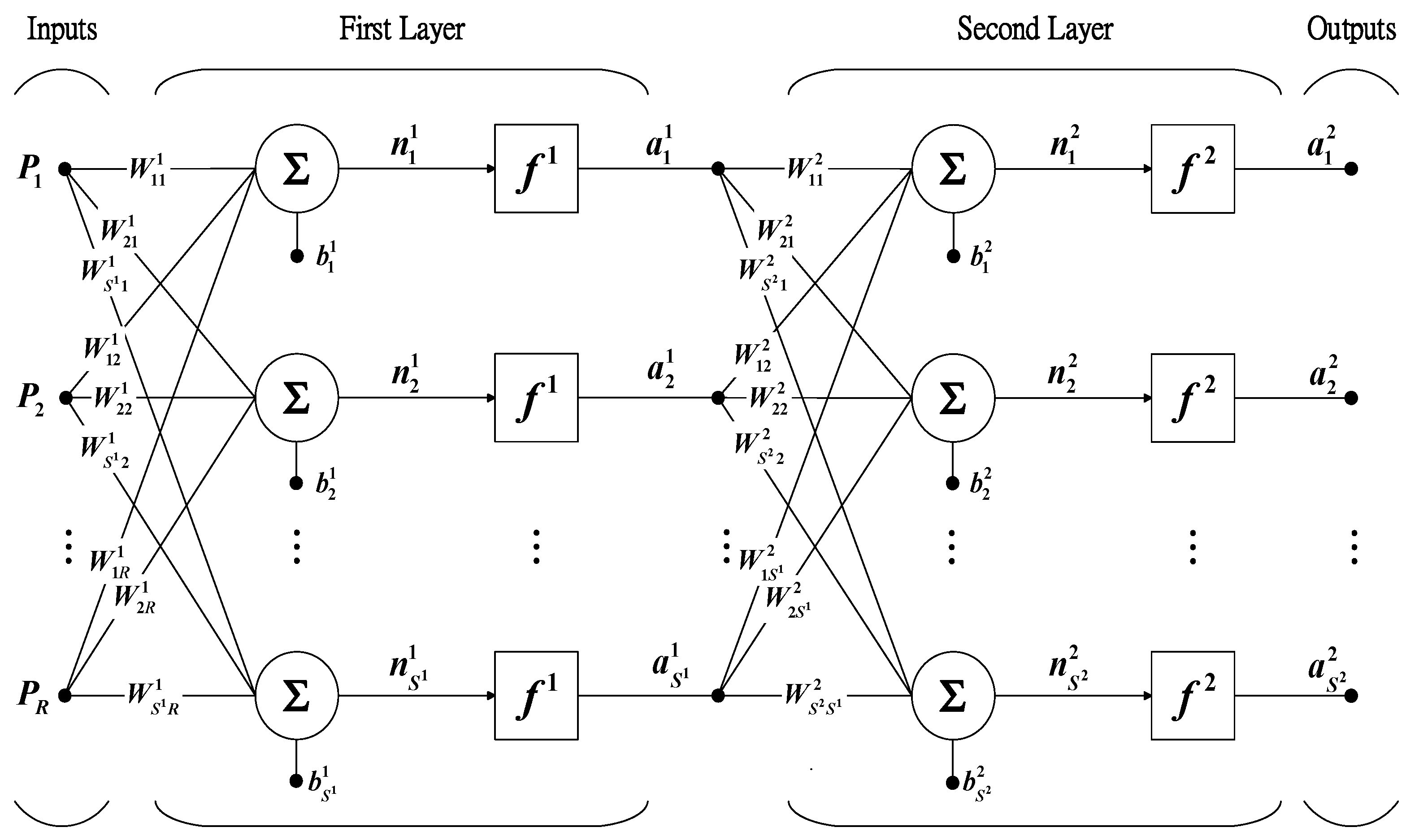
Based on the mixed TBT, a weak-form formulation for a large amplitude free vibration analysis of moderately thick FG rectangular beams under various boundary conditions was developed in this section. The symbols L, h, and b denote the FG beam’s length, thickness, and width. In addition, a set of Cartesian coordinates (x, y, z) for the kinematics description of the FG beam was located at the mid-surface of its left end.
The structural behavior of the FG beam was described using a mixed TBT [39,40,41,42], in which the shear deformation effects were considered to be a constant through the thickness direction of the FG beam, and the related displacement field was given, as follows:
u x x ,   z = u x z ϕ x ,
u y x ,   z = 0 ,
u z x ,   z = w x ,
where u i x ,   z (i = x, y, and z) denote the displacement components of the FG beam in the x, y, and z directions, respectively. u x and w x stand for the mid-plane displacement components of the FG beam in the x and z directions and ϕ x is the total rotation in the xz plane.
The strain-displacement relations of the FG beam considering the VKGN effect were given by:
ε x = u , x z   ϕ , x + 1 / 2 w , x 2 ,
γ x z = ϕ + w , x ,
ε y = ε z = γ y z = γ x y = 0 ,
where ε x ,   ε y ,   ε z ,   γ x z ,   γ y z   and   γ x y are the strain components of the FG beam, and g , x = g / x , in which g = u ,     w ,     and     ϕ .
The nonzero stress components of the FG beam were given by:
σ x = E u , x z   ϕ , x + 1 / 2 w , x 2 ,
τ x z =   k c   G ϕ + w , x ,
where G and E are defined as the shear and Young’s moduli of the FG beam, respectively, and in general, these are specific functions of z, i.e., G = G z and E = E z . k c denotes the shear stress correction factor of the FG beam, which was taken as 5/6 in this work.
The generalized force resultants, namely the axial force N , moment M , and shear force Q , of the FG beam, were defined by:
N = A x x   u , x B x x   ϕ , x + ( A x x / 2 ) w , x 2 ,
M = B x x   u , x + D x x   ϕ , x ( B x x / 2 ) w , x 2 ,
Q = k c   A x z ϕ + w , x ,
where for an N l layered FG beam:
A x x = m = 1 N l   b   z m 1 z m   E z   d z ,       B x x = m = 1 N l   b   z m 1 z m   E z   z   d z ,       D x x = m = 1 N l   b   z m 1 z m   E z   z 2   d z ,       A x z = m = 1 N l   b   z m 1 z m   G z   d z ,
where N l denotes the total number of layers constituting the multi-layered beam, and zm and zm − 1 are the thickness coordinates of the top and bottom surfaces of the mth-layer when measured from the mid-surface of the FG beam.
Four different boundary conditions of the FG beam were considered as follows:
Case 1. S-S supported:
u = w = M = 0           at   x = 0   and   x = L ;
Case 2. C-S supported:
u = w = ϕ = 0           at   x = 0 , and   u = w = M = 0           at   x = L ;
Case 3. C-C supported:
u = w = ϕ = 0           at   x = 0   and   x = L ;
Case 4. C-F supported:
u = w = ϕ = 0           at   x = 0 , and   N = M = Q = 0           at   x = L .
Based on Hamilton’s principle, a weak-form formulation was derived using a variational approach, in which the RMVT combined with the TBT and VKGN kinematics was used. The energy functional of the FG beam could be written in the form of:
I = t 1 t 2 T Π R   d t ,
where T and Π R represent the kinetic energy and Reissner’s potential energy of the FG beam, respectively, and can be given by:
T = e = 1 N e x e x e + 1 1 / 2 m 0   u ( e ) / t 2 + 1 / 2 m 2 ϕ ( e ) / t 2   + 1 / 2 m 0 w ( e ) / t 2 m 1 u ( e ) / t ϕ ( e ) / t d x ,
Π R = e = 1 N e x e x e + 1   N ( e ) u ( e ) , x + 1 / 2 w ( e ) , x 2 + M ( e )   ϕ ( e ) , x + Q ( e ) ϕ ( e ) w ( e ) , x S A x x / 2 N ( e ) 2 S D x x / 2 M ( e ) 2                                                         S B x x N ( e ) M ( e ) 1 / 2 k c A x z Q ( e ) 2 d x + N ¯ 0   u 0 N ¯ L   u L + M ¯ 0 ϕ 0 M ¯ L ϕ L V ¯ 0 w 0 + V ¯ L w L ,
where the superscript e denotes a typical beam element, Ne denotes the total number of beam elements constituting the FG beam; m 0 , m 1 , and m 2 are the mass of the cross-sectional area and its moment of inertia, and are given by m 0 = A   ρ   d A , m 1 = A   ρ   z   d A , and m 2 = A   ρ   z 2   d A ; δ k l is the Kronecker delta symbol, in which δ k l = 1 when k = l , while δ k l = 0 when k l ; S A x x = D x x / A x x D x x B x x B x x , S B x x = B x x / A x x D x x B x x B x x , and S D x x = A x x / A x x D x x B x x B x x ; when the material properties constituting the FG beam were symmetric with respect to the mid-surface, B x x = 0 ; otherwise, B x x 0 . In addition, the variables, N ¯ 0 , N ¯ L , M ¯ 0 ,   M ¯ L ,   V ¯ 0   ,   and   V ¯ L , represented the applied axial forces, moments, and shear forces of the FG beam at the edges.
Based on the RMVT-based TBT, the generalized displacement variables u ( e ) , w ( e ) ,   and   ϕ ( e ) and the generalized force resultant variables N ( e ) ,     M ( e ) ,       and     Q ( e ) of each element were selected as the primary variables subject to variation, and the time function of each field variable was assumed to be the harmonic function, i.e., F ( e ) x ,   z ,   t = F ˜ ( e ) x ,   z   e i   ω   t , in which t represents the time variable, and ω is the natural frequency of the FG beam. Then, by applying Hamilton’s principle and imposing the continuity conditions at the nodes of the beam element, the authors finally obtained the motion equations of the loaded FG beam, as follows:
e = 1 N e   0 0 0 k 14 ( e ) 0 0 0 0 0 0 0 k 26 ( e ) 0 0 0 0 k 35 ( e ) k 36 ( e ) k 41 ( e ) 0 0 k 44 ( e ) k 45 ( e ) 0 0 0 0 k 54 ( e ) k 55 ( e ) 0 0 k 62 ( e ) k 63 ( e ) 0 0 k 66 ( e ) ( m )   + 0 0 0 0 0 0 0 g 22 ( e ) 0 0 0 0 0 0 0 0 0 0 0 g 42 ( e ) 0 0 0 0 0 0 0 0 0 0 0 0 0 0 0 0 ( m 1 ) ω 2   m 11 ( e ) 0 m 13 ( e ) 0 0 0 0 m 22 ( e ) 0 0 0 0 m 31 ( e ) 0 m 33 ( e ) 0 0 0 0 0 0 0 0 0 0 0 0 0 0 0 0 0 0 0 0 0 ( m ) u j ( e ) w j ( e ) ϕ j ( e ) N j ( e ) M j ( e ) Q j ( e )   i = j = 1 , ,   n d ( m ) = e = 1 N e   0 0 0 0 0 0 ( m ) i = 1 , ,   n d ,  
where k   i j ( e ) ,     g   i j ( e )   and     m   i j ( e ) are relevant coefficients and the superscripts m and (m − 1) refer to the mth and (m − 1)th iterative processes.
Based on the linear vibration theory without considering the VKGN, the linear natural frequencies of the FE beam, which were independent of the modal variables, could be obtained by letting the geometrical stiffness coefficients be zero (i.e., g   i j ( e ) = 0). Then, the corresponding eigenvectors were scaled up by allowing the maximum transverse displacement of the FG beam to be identical to a given vibration amplitude w ¯ max , and g   i j ( e ) could be determined using these scaled-up eigenvectors. The nonlinear natural frequencies of the FG beam, which were dependent upon the modal variables, could thus be obtained using the updated eigenvalue system equations (Equation (19)). The iteration process ended when the relative error between the nonlinear frequencies of mth and (m − 1)th iterations were less than 10−5.
Using Equation (19) and the above-mentioned iterative process, the authors could investigate the large amplitude free vibration characteristics of moderately thick FG beams under different boundary conditions.

3. The MP BPNN

3.1. Feeding Forward Process

An MP BPNN was developed and briefly described in this section. For illustrative purposes, a schematic for the structure of the Nh- layer network is shown in Figure 1, in which Nh = 2; p j     j = 1 , ,   R denotes the R inputs; w i j m   is the weight representing the connection to the ith-neuron of the mth-layer from the jth-neuron of the (m − 1)th-layer, such that m = 1,…, Nh, i = 1,…, Sm and j = 1,…, S(m − 1), as well as Sm, which is the total number of neurons used in the mth-layer; b j m is the bias of the jth-neuro of the mth-layer; n i m denotes the net input of the ith-neuron of the mth-layer; n i m = j = 1 S ( m 1 ) w i j m a j ( m 1 ) + b j m ; a i m i = 1 , ,   S m is the ith-output of the mth-layer, and a i m   = f m n i m , where f m is the transfer function used in the mth-layer, and a j 0   = p j . A symbol of R-S1-S2 in this work was thus used to represent a two-layer network algorithm with R inputs, S1 and S2 neurons in the first and second layers, and S2 outputs, in which the number of neurons used for the last layer was the same as the number of final outputs.
For a multilayer network, the output of one layer became the input to the following layer, the operation of which as thus given as:
a m + 1 = f m + 1 n m + 1 = f m + 1 W m + 1 a m + b m + 1       for   m = N h , ,   1 ,   0 ,
where b m + 1 = b   1 m + 1 b   2 m + 1 b S m + 1 m + 1 T ; n m + 1 = n   1 m + 1 n   2 m + 1 n S m + 1 m + 1 T . In this work, the transfer function for the hidden layers of m = 1,…, (Nh − 1) was selected as the log-sigmoid function, while the last output layer of m = Nh was selected as the linear transfer function, such that f m + 1 = f   1 m + 1 f   2 m + 1 f S m + 1 m + 1 T , in which f   i m + 1 = 1 / 1 + e n   i m + 1 and f i N h = n i N h .
In the first hidden layer, the neurons received external inputs as follows:
a 0 = p ,
where p = p 1 p 2 p R , which provided the starting point for Equation (21).
The outputs of the neurons in the last layer were considered as the network outputs and defined as:
a = a N h .

3.2. Backpropagation Process

In order to operate the algorithm, there were appropriate input data sets and their corresponding target output sets, which were provided and given as:
p 1 ,     t 1 ,   p 2 ,     t 2 ,   p q ,     t q ,   ,   p Q ,     t Q .
The learning rule used in this ANN algorithm is called the least mean square algorithm, which means that the network parameters could be adjusted to minimize the mean square error as follows:
Min         F ^ x = q = 1 Q t q a q T t q a q = q = 1 Q e q T e q = q = 1 Q j = 1 S N h e j q 2 = i = 1 n e v i 2 ,
where x = w 11 1 , ,   w S 1   R 1 ,   b 1 1 , ,   b S 1 1 , ,   w 11 N h , ,   w S N h   S N h 1 N h , b   1 N h , ,   b S N h N h   , in which the total number (np) for the parameters, including all the weights and biases in this MP BPNN algorithm, is n p = R + 1 S 1 + S 1 + 1 S 2 + S N h 1 + 1 S N h . v T = v 1     v 2         v n e   = e 11     e 21     e S N h   1   e 12     e 22     e S N h   2     e S N h   Q , in which the total number (ne) of the square error terms is n e = Q   S N h .
In order to speed up the convergence rate, the Levenberg–Marquardt algorithm [26] was adopted for network training.
When the input P q was fed into the network and the corresponding network output a q N h was computed, the Levenberg–Marquardt BP algorithm could be initialized with:
S ˜   N h = S ˜     1   N h S ˜     2   N h S ˜     Q   N h
where S ˜   q N h = F ˙ N h n   q N h , and the dimension of F ˙ m n m is S m x S m and that of S ˜ m is S m × Q   S m for m = 1,…, Nh.
The total Marquardt sensitivity matrices S ˜   m could then be obtained in the following order: m = Nh − 1, Nh − 2, …, 1, using the BP network, and this could be written as follows:
S ˜   m = S ˜     1   m S ˜     2   m S ˜     Q   m       for   m = N h 1 ,   N h 2 , ,   1 ,
where S ˜ q   m = F ˙   m n   q m   W m + 1 T   S ˜   q   m + 1 for q = 1,…, Q.
According to the Levenberg–Marquardt BP algorithm, all of the parameters could be modified using an iteration process as follows:
X ( k + 1 ) = X ( k ) J T x ( k ) J x ( k ) + μ ( k )   I 1   J T x ( k ) v x ( k ) ,
where k denotes the number of iterations, and the initial value of μ , i.e., μ ( 0 ) , was taken to be a significant value (e.g., μ ( 0 ) = 10,000). If a step yielded a more significant value for F(x), then the step was repeated with μ ( k ) multiplied by a factor ϑ > 1 (e.g., ϑ = 2 in this work), and if a step yielded a smaller value for F(x), then the step was repeated with μ ( k ) divided by a factor ϑ > 1 (e.g., ϑ = 3 in this work). Eventually, the iteration process converged. In this work, the stop criteria of the iteration process were considered as follows:
(1)
When the root of the mean square relative error Re was less than 10−5, i.e.,
R e = q = 1 Q t q a q T t q a q / t q T t q / ( Q   S N h ) 10 5
(2)
When the number of iterations was greater than 20,000.

4. Illustrative Examples

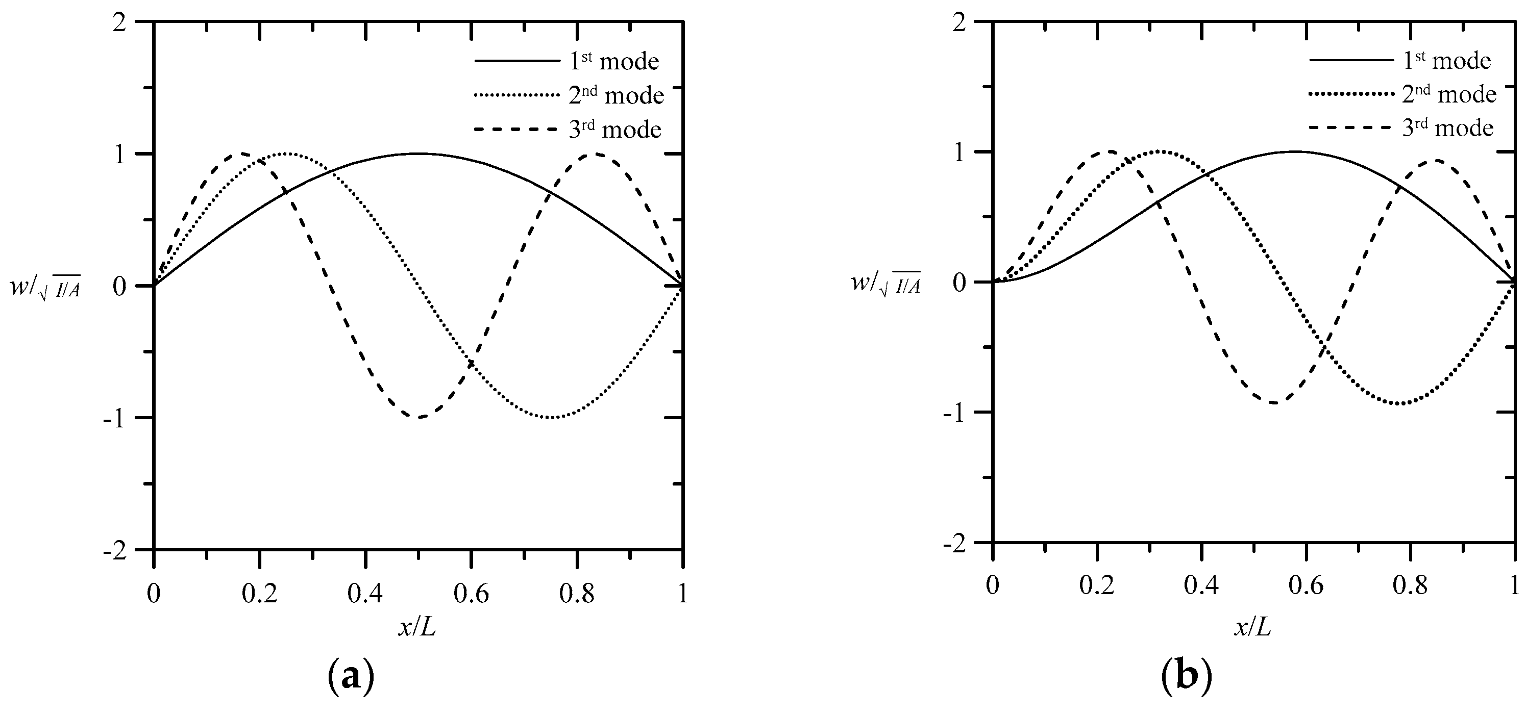
4.1. Large Amplitude-Free Vibration Analysis Using the Mixed FE Method

In this section, the authors investigate the large amplitude-free vibration behavior of homogeneous isotropic and FG isotropic beams with combinations of simply supported, free, and clamped boundary conditions using the mixed FE method.
Table 1 shows the results of the convergence study for the mixed FE solutions of the nonlinear-to-linear natural frequency ratios ( ω n l / ω l i n e a r ) of homogeneous isotropic beams under S-S boundary conditions. This issue has also been studied using various FE methods, such as the Lagrange-type FE method [43] and the Galerkin FE method [44]. The accuracy and convergence rate of the RMVT-based FE methods with different orders used to expand the primary variables in the element domain could thus be validated by comparing their solutions with those available in the literature.
The geometric parameters of the beams were L/h = 20 and h = 0.1 m. The material properties were E = 322.3     GPa , and υ = 0.24 . A maximum dimensionless amplitude was defined as obtaining the nonlinear natural frequencies of the beams.
It can be seen in Table 1 that the RMVT-based (or mixed) FE solutions converged rapidly and that convergent solutions were obtained when the 16 linear, eight quadratic or four cubic elements were used. Moreover, the convergent solutions were in excellent agreement with those obtained using various PVD-based FE methods [43,44].
Table 2 compares the mixed FE solutions for the natural frequency ratios of FG beams under C-C boundary conditions with the solutions reported in the literature, in which 16 cubic elements were used. In addition, mixed FE solutions for the S-S, C-S, and C-F boundary conditions were also presented. The FG beam was made of a ceramic-metal two-phase material, comprised Silicon nitride Si3N4 (ceramic) and a stainless steel SuS304 (metal), and the material properties of the Si3N4 and SuS304 materials were E c = 322.3     GPa , υ c = 0.24 , and ρ c = 2370     K g / m 3 , as well as E m = 207.8     GPa , υ m = 0.3178   , and ρ m = 8166     K g / m 3 , in which the subscripts c and m denoted the ceramic and metal materials, respectively. The material properties of the FG beam were assumed to obey the power-law distributions through the thickness direction according to the volume fractions of the constituents, which were Γ c z = 1 / 2 + z / h κ p and Γ m z = 1 Γ c z , in which κ p represents the material-property gradient index, and the effective material properties of this were estimated using the rule of mixture, as follows:
P z = P c Γ c z + P m Γ m z
where P represents E, υ , and ρ .
It can be seen in Table 2 that the nonlinear-to-linear natural frequency ratios increased when the maximum dimensionless amplitude became greater for C-C, C-S, and S-S boundary conditions. Again, it can be seen in Table 2 that for the C-C boundary conditions, the mixed FE solutions closely agreed with the solutions obtained by Elmaguiri et al. [45] and Ke et al. [46] with Euler-Bernoulli’s beam theory accounting for the VKGN effect. These results also show that the magnitudes of the nonlinear-to-linear natural frequency ratio at increments for different boundary conditions were arranged in descending order: S-S boundary conditions > C-S boundary conditions> C-C boundary conditions.
On the other hand, for C-F boundary conditions, the nonlinear-to-linear natural frequency ratios slightly decreased when the maximum dimensionless amplitude became greater. This was because the geometrical nonlinearity effect and the boundary constraints resulted in an axial tensional force for the S-S, C-S, and C-C boundary conditions, enhancing the overall stiffness of the FG beams. In contrast, this resulted in a very small compressive force for the C-F boundary conditions, which slightly weakened the overall stiffness of the FG beams. The results also showed that the influence of the geometrical nonlinearity effect on the natural frequencies of the FG beams for different boundary conditions was arranged in descending order: S-S > C-S > C-C > C-F boundary conditions.
The modal shapes of the FG beam under different boundary conditions are shown in Figure 2, in which the maximum dimensionless amplitude and the material-property gradient index were taken to be w ¯ max = w max / I / A = 1 and κ p = 0.3, respectively.

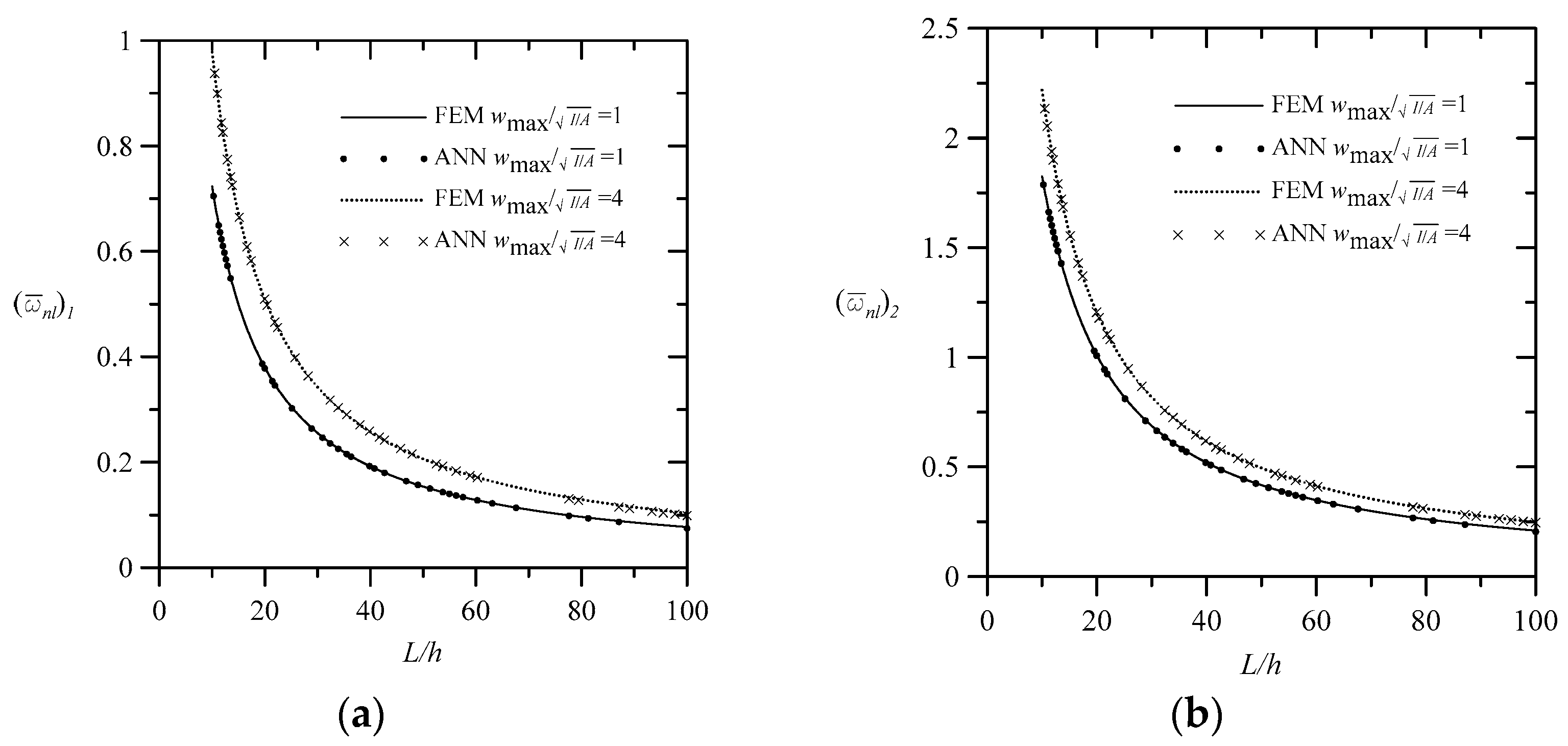
4.2. Large Amplitude–Free Vibration Analysis Using the Developed MP BPNN

In this section, the large amplitude free vibration analysis of the FG rectangular beams mentioned above was undertaken again using the developed MP BPNN algorithm, which was trained using the mixed FE solutions. The boundary conditions of the FG beams were considered to be clamped-clamped edge conditions. The cross-section of the FG beam was 10 cm × 10 cm, and their material properties were considered the same as those used in Table 2. The dimensionless nonlinear frequency parameter was defined as ω ¯ n l = ω n l   ρ m   L 2 / E m .
After training, a set of optimal parameters, including the weight numbers w i j m and biases b j m , where i = 1,…, Sm, j = 1,…, S(m − 1), and m = 1,…, Nh, could be obtained, and the trained MP BPNN could replace the mixed FE method to predict the nonlinear natural frequencies of the FG beams significantly faster compared to the case with the mixed FE method. In the training of this MP BPNN, R was taken as three and represented the length-to-thickness ratio (L/h), the material-property gradient index ( κ p ), and the maximum dimensionless amplitude ( w max /   I / A ), in which L/h = 10 1 + 0.05 i , i = 0,…, 20; κ p = 10 2 + 0.2 i , i = 0,…, 20; w max /   I / A = 1 + i, i = 0,…, 3, such that the total number of the training data sets was 21 × 21 × 4 = 1764. The number of outputs was taken as two, which were the first and second lowest natural frequencies of the FG beams. Thus, there were 1764 training data sets for the first lowest and second lowest nonlinear natural frequencies of the FG beams, which were obtained using the mixed FE methods and used to train the n p parameters for each MP BPNN, in which n p = R + 1 S 1 + S 1 + 1 S 2 + S N h 1 + 1 S N h , the initial values of which were randomly generated between −1 and 1. There were 100 sets of the initial values of the np parameters used for each MP BPNN algorithm in this analysis, for which the first three best results are shown in Table 3 and were estimated using the Re of the outputs compared to the other 200 selected testing data.
In this section, the large amplitude free vibration analysis of FG rectangular beams mentioned above was undertaken again using the developed MP BPNN algorithm, which was trained using the mixed FE solutions. The FG beams’ boundary conditions were considered clamped-clamped edge conditions. The cross-section of the FG beam was 10 cm × 10 cm, and their material properties were considered the same as those used in Table 2. The dimensionless nonlinear frequency parameter was defined as ω ¯ n l = ω n l   ρ m   L 2 / E m .
After training, a set of optimal parameters, including the weight numbers w i j m and biases b j m , where i = 1,…, Sm, j = 1,…, S(m  1), and m = 1,…, Nh, could be obtained, and the trained MP BPNN replaced the mixed FE method to predict the nonlinear natural frequencies of the FG beams significantly faster compared to the case with the mixed FE method. In the training of this MP BPNN, R was taken as three, and represented the length-to-thickness ratio (L/h), the material-property gradient index ( κ p ), and the maximum dimensionless amplitude ( w max /   I / A ), in which L/h = 10 1 + 0.05 i , i = 0,…, 20; κ p = 10 2 + 0.2 i , i = 0,…, 20; w max /   I / A = 1 + i, i = 0,…, 3, such that the total number of the training data sets was 21 × 21 × 4 = 1764. The number of outputs was taken as two, which were the first and second lowest natural frequencies of the FG beams. Thus, there were 1764 training data sets for the first lowest and second lowest nonlinear natural frequencies of the FG beams obtained using the mixed FE methods, and these were used to train the n p parameters for each MP BPNN, in which n p = R + 1 S 1 + S 1 + 1 S 2 + S N h 1 + 1 S N h , the initial values of which were randomly generated between −1 and 1. There were 100 sets of the initial values of the np parameters used for each MP BPNN algorithm in this analysis, for which the first three best results are shown in Table 3; these were estimated using the Re of outputs as compared with another 200 selected testing data.
It can be seen in Table 3 that the 3-6-6-2 and 3-4-4-4-2 BPNN algorithms yielded optimal results, for which the values of Re were 0.0006% and 0.0008%, respectively. The 3-6-6-2 BPNN algorithm was thus used to predict the first lowest and second lowest nonlinear natural frequencies of the FG beams, as shown in Figure 3 and Figure 4. Furthermore, it can be seen in each curve of Figure 3 and Figure 4 that the solutions obtained using the mixed FE method, drawn using the solid lines and the developed MP BPNN algorithm, and drawn using the discrete symbols closely agreed with each other for a randomly selected group of 50 sets of input data.
Table 4 compares the computer execution time required for the developed MP BPNN and the mixed FE method when randomly selecting 50 input data sets, as shown in Figure 3 and Figure 4. It was shown that the central processing unit (CPU) time required for the mixed FE method was about 2800 times greater than that needed for the developed MP BPNN algorithm. Thus, the trained MP BPNN algorithm was superior to the mixed FE method because it was less time-consuming.
The results also showed that the nonlinear frequency parameters decreased when the length-to-thickness ratio increased. The nonlinear frequency parameters depended on the maximum dimensionless amplitude, and these values increased when the maximum dimensionless amplitude was greater.

5. Conclusions

In this article, based on the RMVT and TBT, a mixed FE method was developed for the nonlinear free vibration analysis of FG beams under the combinations of simply supported, free, and clamped edge conditions. Implementing the mixed FE method shows that its convergent solutions were obtained when 16 linear, eight quadratic, or four cubic elements were used and that these convergent solutions were in excellent agreement with the accuracy solutions reported in the literature. These results also indicated that the nonlinear natural frequency-to-linear natural frequency ratios increased when the maximum dimensionless amplitude increased. On the other hand, for C-F boundary conditions, the nonlinear-to-linear natural frequency ratios decreased when the maximum dimensionless amplitude became greater. The influence of the geometrical nonlinearity effect on the natural frequencies of the FG beams for different boundary conditions was arranged in descending order: S-S > C-S > C-C > C-F boundary conditions.
An MP BPNN algorithm was also developed, in which the Levenberg–Marquardt algorithm was used to speed up MP BPNN’s convergence rate. After training using the mixed FE solutions, it was shown that the trained MP BPNN algorithm was superior to the mixed FE method because it was approximately 1/2800 times less time-consuming. It is worth mentioning that the above comparison did not account for the cost of generating FEM data and training the BPNN. It is expected that the developed MP BPNN algorithm could be extended to research subjects, including inverse problems, optimal design, structural control, etc., when the traditional analytical or numerical methods used in such studies are very time-consuming. Therefore, applying the MP BPNN to the research mentioned above is ongoing.

Author Contributions

Conceptualization, C.-P.W.; methodology, C.-P.W.; software, S.-T.Y. and J.-H.L.; validation, C.-P.W., S.-T.Y. and J.-H.L.; formal analysis, C.-P.W.; investigation, C.-P.W.; resources, C.-P.W.; data curation, S.-T.Y. and J.-H.L.; writing—original draft preparation, C.-P.W.; writing—review and editing, C.-P.W.; visualization, C.-P.W.; supervision, C.-P.W. All authors have read and agreed to the published version of the manuscript.

Funding

This research received no external funding.

Institutional Review Board Statement

Not applicable.

Informed Consent Statement

Not applicable.

Data Availability Statement

The data supporting reported results can be found at https://drive.google.com/drive/folders/1TmbVHAdo6sZNMGytFrmZPrLPL4_Ye4aN?usp=share_link (accessed on 1 May 2023).

Conflicts of Interest

The authors declare no conflict of interest.

References

  1. Koizumi, M. Recent progress of functionally graded materials in Japan. Ceram. Eng. Sci. Proc. 1992, 13, 333–347. [Google Scholar]
  2. Koizumi, M. FGM activities in Japan. Compos. Part B 1997, 28, 1–4. [Google Scholar] [CrossRef]
  3. Jha, D.K.; Kant, T.; Singh, R.K. A critical review of recent research on functionally graded plates. Compos. Struct. 2013, 96, 833–849. [Google Scholar] [CrossRef]
  4. Shen, H.S. Functionally Graded Materials: Nonlinear Analysis of Plates and Shells; CRC Press: Boca Raton, FL, USA, 2009. [Google Scholar]
  5. Chakraborty, A.; Mahapatra, D.R.; Gopalakrishnan, S. Finite element analysis of free vibration and wave propagation in asymmetric composite beams with structural discontinuities. Compos. Struct. 2002, 55, 23–36. [Google Scholar] [CrossRef]
  6. Chakraborty, A.; Gopalakrishnan, S.; Reddy, J.N. A new beam finite element for analyzing functionally graded materials. Int. J. Mech. Sci. 2003, 45, 519–539. [Google Scholar] [CrossRef]
  7. Aydogdu, M.; Taskin, V. Free vibration analysis of functionally graded beams with simply supported edges. Mater. Des. 2007, 28, 1651–1656. [Google Scholar] [CrossRef]
  8. Simsek, M. Static analysis of a functionally graded beam under a uniformly distributed load by Ritz method. Int. J. Eng. Appl. Sci. 2009, 1, 1–11. [Google Scholar]
  9. Simsek, M. Fundamental frequency analysis of functionally graded beams using different higher-order beam theories. Nucl. Eng. Des. 2010, 240, 697–705. [Google Scholar] [CrossRef]
  10. Ebrahimi, F.; Farazmandnia, N. Thermo-mechanical vibration analysis of sandwich beams with functionally graded carbon nanotube-reinforced composite face sheets based on a higher-order shear deformation beam theory. Mech. Adv. Mater. Struct. 2017, 24, 820–829. [Google Scholar] [CrossRef]
  11. Carrera, E. Theories and finite elements for multilayered plates and shells: A unified compact formulation with numerical assessment and benchmarking. Arch. Comput. Methods Eng. 2003, 10, 215–296. [Google Scholar] [CrossRef]
  12. De Pietro, G.; Hui, Y.; Giunta, G.; Belouettar, S.; Carrera, E.; Hu, H. Hierarchical one-dimensional finite elements for the thermal stress analysis of three-dimensional functionally graded beams. Compos. Struct. 2016, 153, 514–528. [Google Scholar] [CrossRef] [Green Version]
  13. Coskun, S.; Kim, J.; Toutanji, H. Bending, free vibration, and buckling analysis of functionally graded porous micro-plates using a general third-order plate theory. J. Compos. Sci. 2019, 3, 15. [Google Scholar] [CrossRef] [Green Version]
  14. Tham, V.V.; Quoc, T.H.; Tu, T.M. Free vibration analysis of laminated functionally graded carbon nanotube-reinforced composite doubly curved shallow shell panels using a new four-variable refined theory. J. Compos. Sci. 2019, 3, 104. [Google Scholar] [CrossRef] [Green Version]
  15. Wu, C.P.; Xu, Z.R. Strong and weak formulations of a mixed higher-order shear deformation theory for the static analysis of functionally graded beams under thermo-mechanical loads. J. Compos. Sci. 2020, 4, 158. [Google Scholar] [CrossRef]
  16. Wu, C.P.; Li, K.W. Multi-objective optimization of functionally graded beams using a genetic algorithm with non-dominated sorting. J. Compos. Sci. 2021, 5, 92. [Google Scholar] [CrossRef]
  17. Ma, L.S.; Lee, D.W. Exact solutions for nonlinear static responses of a shear deformable FGM beam under an in-plane thermal loading. Eur. J. Mech. A/Solids 2012, 31, 13–20. [Google Scholar] [CrossRef]
  18. Zhang, D.G. Nonlinear bending analysis of FGM beams based on physical neutral surface and high order shear deformation theory. Compos. Struct. 2013, 100, 121–126. [Google Scholar] [CrossRef]
  19. Salami, S.J. Extended high order sandwich panel theory for bending analysis of sandwich beams with carbon nanotube reinforced face sheets. Phys. E 2016, 76, 187–197. [Google Scholar] [CrossRef]
  20. Shen, H.S. Nonlinear bending of functionally graded carbon nanotube-reinforced composite plates in thermal environments. Compos. Struct. 2009, 91, 9–19. [Google Scholar] [CrossRef]
  21. Ghayesh, M.H. Nonlinear vibrations of axially functionally graded Timoshenko tapered beams. J. Comput. Nonlinear Dyn. 2018, 13, 041002. [Google Scholar] [CrossRef]
  22. Shen, H.S.; Lin, F.; Xiang, Y. Nonlinear vibration of functionally graded graphene-reinforced composite laminated beams resting on elastic foundations in thermal environments. Nonlinear Dyn. 2017, 90, 899–914. [Google Scholar] [CrossRef]
  23. Ding, J.; Chu, L.; Xin, L.; Dui, G. Nonlinear vibration analysis of functionally graded beams considering the influences of the rotary inertia of the cross section and neural surface position. Mech. Based Des. Struct. Mach. 2018, 46, 225–237. [Google Scholar] [CrossRef]
  24. Eltaher, M.A.; Mohamed, N.; Mohamed, S.A.; Seddek, L.F. Periodic and nonperiodic modes of postbuckling and nonlinear vibration of beams attached to nonlinear foundations. Appl. Math. Model. 2019, 75, 414–445. [Google Scholar] [CrossRef]
  25. Chaudhari, V.K.; Lal, A. Nonlinear free vibration analysis of elastically supported nanotube-reinforced composite beam in thermal environment. Procedia Eng. 2016, 144, 928–935. [Google Scholar] [CrossRef] [Green Version]
  26. Mirzaei, M.; Kiani, Y. Nonlinear free vibration of temperature-dependent sandwich beams with carbon nanotube-reinforced face sheets. Acta Mech. 2016, 227, 1869–1884. [Google Scholar] [CrossRef]
  27. Babaei, H.; Kiani, Y.; Eslami, M.R. Large amplitude free vibrations of FGM beams on nonlinear elastic foundation in thermal field based on neutral/mid-plane formulations. Iran. J. Sci. Technol. Trans. Mech. Eng. 2021, 45, 611–630. [Google Scholar] [CrossRef]
  28. Hagan, M.T.; Demuth, H.B.; Beale, M. Neural Network Design; PWS Pub. Comp.: New York, NY, USA, 1995. [Google Scholar]
  29. Yagawa, G.; Okuda, H. Neural networks in computational mechanics. Arch. Comput. Methods Eng. 1996, 3, 435–512. [Google Scholar] [CrossRef]
  30. Zhang, Z.; Friedrich, K. Artificial neural networks applied to polymer composites: A review. Compos. Sci. Technol. 2003, 63, 2029–2044. [Google Scholar] [CrossRef]
  31. Ootao, Y.; Kawamura, R.; Tanigawa, Y.; Nakamura, T. Neural network optimization of material composition of a functionally graded material plate at arbitrary temperature range and temperature rise. Arch. Appl. Mech. 1998, 68, 662–676. [Google Scholar] [CrossRef]
  32. Ootao, Y.; Kawamura, R.; Tanigawa, Y.; Imamura, R. Optimization of material composition of nonhomogeneous hollow circular cylinder for thermal stress relaxation making use of neural network. J. Therm. Stress. 1999, 22, 1–22. [Google Scholar]
  33. Chakraverty, S.; Singh, V.P.; Sharma, R.K. Regression based weight generation algorithm in neural network for estimation of frequencies of vibrating plates. Comput. Methods Appl. Mech. Eng. 2006, 195, 4194–4202. [Google Scholar] [CrossRef]
  34. Reddy, M.R.S.; Reddy, B.S.; Reddy, V.N.; Sreenivasulu, S. Prediction of natural frequency of laminated composite plates using artificial neural networks. Engineering 2012, 4, 329–337. [Google Scholar] [CrossRef] [Green Version]
  35. Jodaei, A.; Jalal, M.; Yas, M.H. Free vibration analysis of functionally graded annular plates by state-space based differential quadrature method and comparative modeling by ANN. Compos. Part B 2012, 43, 340–353. [Google Scholar] [CrossRef]
  36. Fetene, B.N.; Shufen, R.; Dixit, U.S. FEM-based neural network modeling of laser-assisted bending. Neural Comput. Appl. 2018, 29, 69–82. [Google Scholar] [CrossRef]
  37. Subramani, T.; Sharmila, S. Prediction of deflection and stresses of laminated composite plate with artificial network aid. Int. J. Modern Eng. Res. 2014, 4, 51–58. [Google Scholar]
  38. Liu, X.; Du, X.; Niu, X. A neural network method applied in prediction eigenvalue buckling for sandwich plates. Inform. Technol. J. 2013, 12, 8129–8134. [Google Scholar]
  39. Reissner, E. On a certain mixed variational theorem and a proposed application. Int. J. Numer. Methods Eng. 1984, 20, 1366–1368. [Google Scholar] [CrossRef]
  40. Carrera, E. An assessment of mixed and classical theories on global and local response of multilayered orthotropic plates. Compos. Struct. 2000, 50, 183–198. [Google Scholar] [CrossRef]
  41. Wu, C.P.; Lai, W.W. Free vibration of an embedded single-walled carbon nanotube with various boundary conditions using the RMVT-based nonlocal Timoshenko beam theory and DQ method. Phys. E 2015, 68, 8–21. [Google Scholar] [CrossRef]
  42. Wu, C.P.; Lai, W.W. Reissner’s mixed variational theorem-based nonlocal Timoshenko beam theory for a single-walled carbon nanotube embedded in an elastic medium and with various boundary conditions. Compos. Struct. 2015, 122, 390–404. [Google Scholar] [CrossRef]
  43. Sarma, B.S.; Varadan, T.K. Lagrange-type formulation for finite element analysis of non-linear beam vibrations. J. Sound Vib. 1983, 86, 61–70. [Google Scholar] [CrossRef]
  44. Bhashyam, G.R.; Prathap, G. Galerkin finite element method for nonlinear beam vibrations. J. Sound Vib. 1980, 72, 191–203. [Google Scholar] [CrossRef]
  45. Elmaguiri, M.N.; Haterbouch, M.; Bouayad, A.; Oussouaddi, O. Geometrically nonlinear free vibration of functionally graded beams. J. Mater. Environ. Sci. 2015, 6, 3620–3633. [Google Scholar]
  46. Ke, L.L.; Yang, J.; Kitipornchai, S. An analytical study on the nonlinear vibration of functionally graded beams. Meccanica 2010, 45, 743–752. [Google Scholar] [CrossRef]
Figure 1. Schematic of the structure of a two-layer network.
Jcs 07 00229 g001
Figure 2. The 1st, 2nd, and 3rd mode shapes of the FG beams under (a) S−S, (b) C−S, (c) C−C, and (d) C−F boundary conditions.
Jcs 07 00229 g002aJcs 07 00229 g002b
Figure 3. Variations in the nonlinear frequency parameters of FG beams with the aspect ratio using the mixed FE method and the developed MP BPNN algorithm for w max / I / A = 1 and 4, and κ p = 4; (a) The first lowest frequency parameters, (b) The second lowest frequency parameter.
Jcs 07 00229 g003
Figure 4. Variations in the nonlinear frequency parameters of FG beams with the aspect ratio using the mixed FE method and the proposed MP BPNN algorithm for κ p = 0.1, 1, and 10, and w max / I / A = 2; (a) The first lowest frequency parameters, (b) The second lowest frequency parameters.
Jcs 07 00229 g004
Table 1. Results of the convergence study for the mixed FE solutions of the nonlinear-to-linear natural frequency ratios of isotropic beams under S-S boundary conditions.
Theories w max / I / A
1.02.03.04.0
Current four linear elements1.11961.41931.81172.2488
Current eight linear elements1.11871.41641.80652.2412
Current 16 linear elements1.1187 1.41631.80622.2407
Current four quadratic elements1.11731.41241.80062.2342
Current eight quadratic elements1.11831.41551.80532.2398
Current 16 quadratic elements1.11861.41611.80612.2406
Current four cubic elements1.11871.41641.80642.2410
Current eight cubic elements1.11871.41621.80622.2407
Sarma and Varadan [43]1.11801.41421.80282.2361
Bhashyam and Prathap [44]1.11801.41411.80272.2359
Table 2. Comparisons between the mixed FE solutions of the nonlinear-to-linear natural frequency ratios ( ω n l / ω l i n e a r ) of FG beams under C-C boundary conditions and the solutions reported in the literature, in which the mixed FE solutions for the S-S, C-S, and C-F boundary conditions are also presented.
Boundary Conditions κ p Theories W ¯ max = W max / I / A
1234
C-C0.3Mixed FE method1.03051.11641.24451.4017
Elmaguiri et al. [45]1.02271.08751.18691.3121
Ke et al. [46]1.02201.08521.18311.3079
1Mixed FE method1.03041.11581.24341.4000
Elmaguiri et al. [45]1.02251.08711.18601.3106
Ke et al. [46]1.00251.08731.18741.3149
2Mixed FE method1.02961.11281.23741.3906
Elmaguiri et al. [45]1.02151.08321.17801.2980
Ke et al. [46]1.02321.09001.19291.3237
S-S0.3Mixed FE method1.14921.46661.86812.3102
1Mixed FE method1.17041.49641.89932.3397
2Mixed FE method1.16951.48991.88552.3182
C-S0.3Mixed FE method1.06961.23791.46671.7299
1Mixed FE method1.07641.24811.47791.7409
2Mixed FE method1.07551.24381.46911.7272
C-F0.3Mixed FE method1.000040.999980.999790.99948
1Mixed FE method1.000081.000040.999890.99961
2Mixed FE method1.000061.000020.999850.99956
Table 3. General information regarding the developed MP BPNNs and their performance.
No. Neurons
of Each Hidden Layer
No. Hidden Layers (i.e., ( N h 1 ) )
1234
No.
Parameters
Training
Time (s)
Re of
Outputs
No. ParametersTraining
Time (s)
Re of
Outputs
No.
Parameters
Training
Time (s)
Re of
Outputs
No.
Parameters
Training
Time (s)
Re of
Outputs
21440.990.2328%20116.500.1913%2683.460.0341%32314.250.0296%
31.980.2331% 170.480.1917% 52.810.1315% 525.970.0569%
32.500.2331% 103.020.2206% 56.060.1426% 107.980.0572%
42645.130.1393%4670.940.0048%66435.870.0008%
25.450.1421% 38.680.0167% 188.260.0043%
35.500.2676% 124.840.0168% 78.460.0128%
638163.320.0237%80173.840.0006%
55.700.0338% 252.950.0007%
55.110.0467% 533.020.0008%
85082.670.0228%
86.690.0266%
122.420.0359%
Table 4. A comparison of the CPU time required for the proposed MP BPNN and the mixed FEM when randomly selecting a group of 50 input data sets is shown in Figure 2 and Figure 3.
[ κ p ,   w max / I / A ] Time (s)
ANNFEM
[4, 1]0.00277.1167
[4, 4]0.00257.5926
[0.1, 2]0.00267.4780
[1, 2]0.00267.0521
CPU: Central processing unit.
Disclaimer/Publisher’s Note: The statements, opinions and data contained in all publications are solely those of the individual author(s) and contributor(s) and not of MDPI and/or the editor(s). MDPI and/or the editor(s) disclaim responsibility for any injury to people or property resulting from any ideas, methods, instructions or products referred to in the content.

