Author Contributions
Conceptualization: A.H., R.S. and N.N.; Methodology: A.H., R.S. and N.N.; Validation: A.H., R.S., N.N., B.R.N.M., M.K., M.N. and D.S.; Formal Analysis: A.H., R.S., N.N., B.R.N.M., M.K., M.N. and D.S.; Writing—original draft preparation: A.H., R.S. and N.N.; writing—review and editing: A.H., R.S., N.N., B.R.N.M., M.K. and M.N.; Visualization: A.H., R.S. and N.N. All authors have read and agreed to the published version of the manuscript.
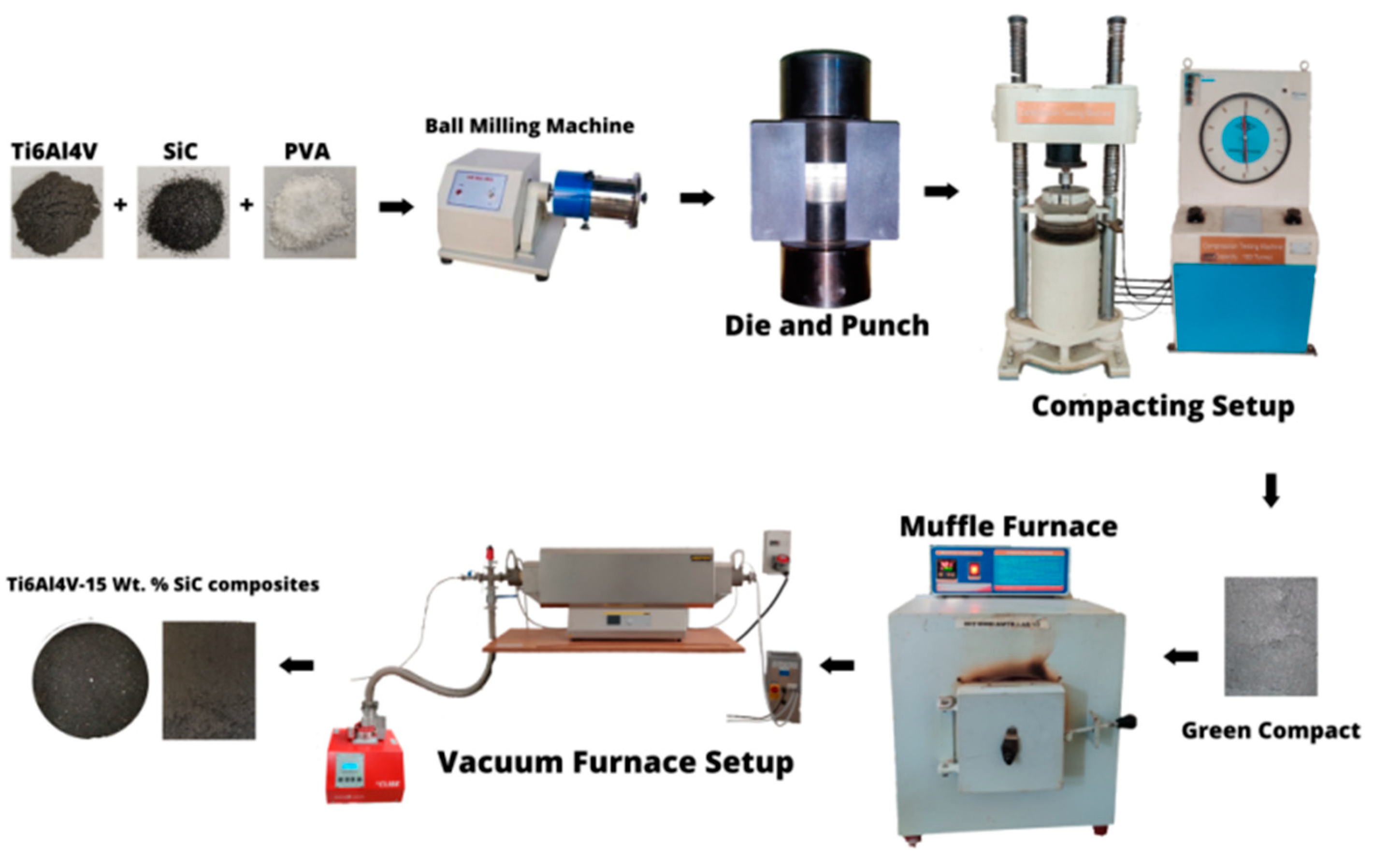
Figure 1.
Flowchart of Titanium Silicon Carbide composite processing [
20].
Figure 1.
Flowchart of Titanium Silicon Carbide composite processing [
20].
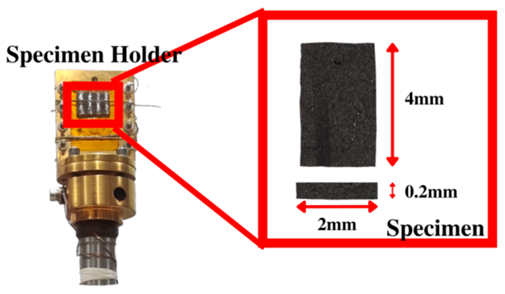
Figure 2.
Workpiece for measuring electrical conductivity.
Figure 2.
Workpiece for measuring electrical conductivity.
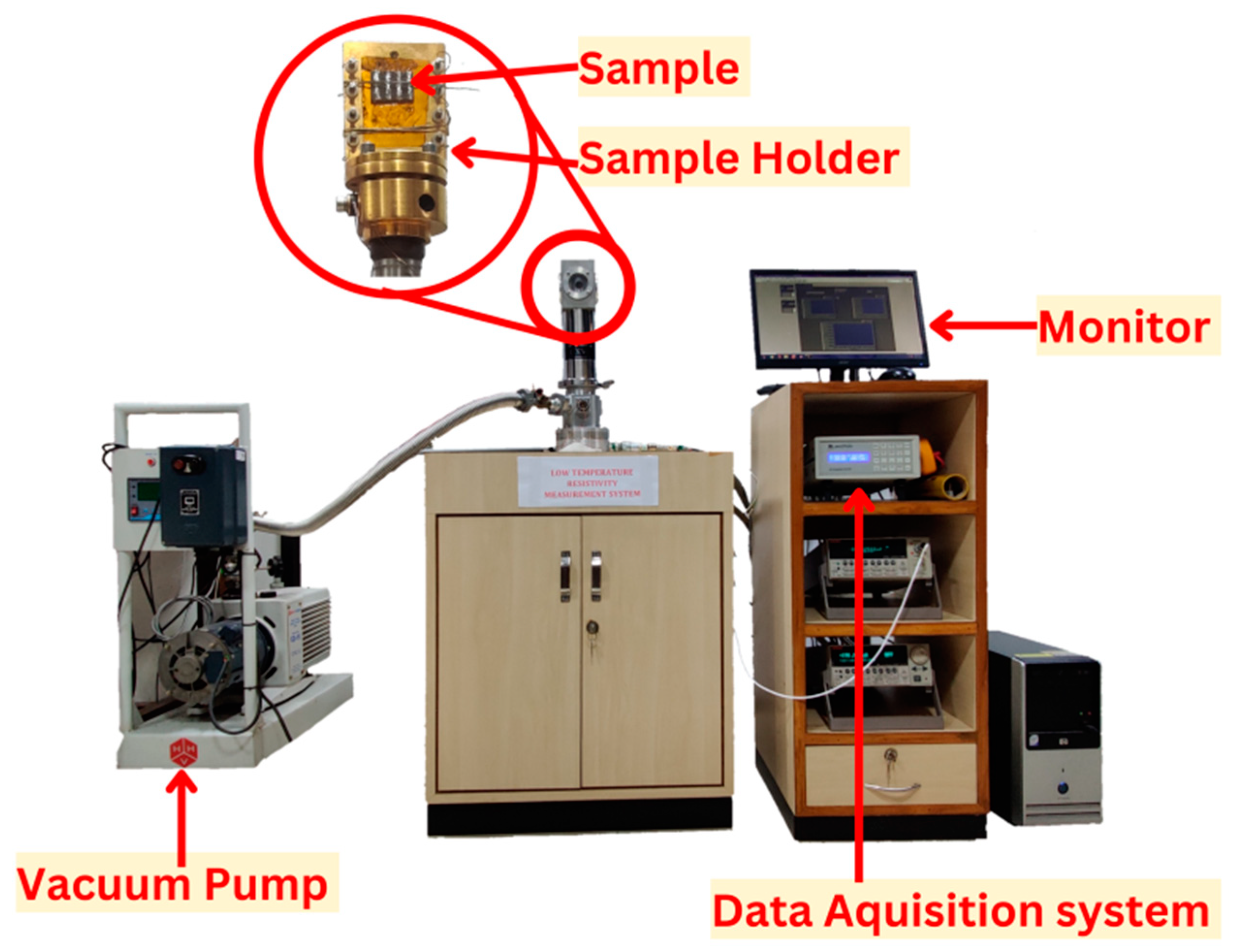
Figure 3.
Keith 400 low-temperature electrical resistivity measuring instrument.
Figure 3.
Keith 400 low-temperature electrical resistivity measuring instrument.
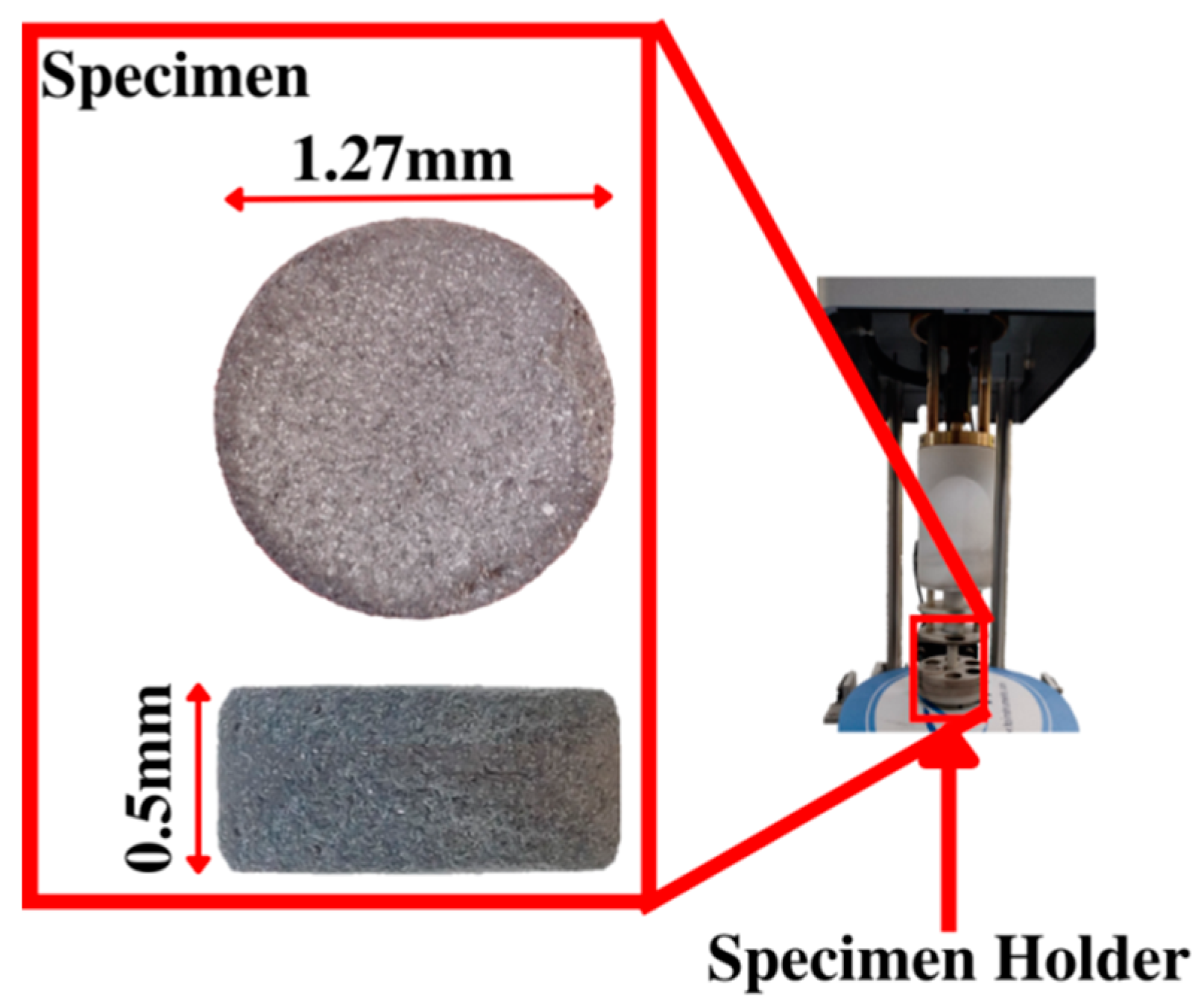
Figure 4.
Workpiece for measuring thermal conductivity.
Figure 4.
Workpiece for measuring thermal conductivity.
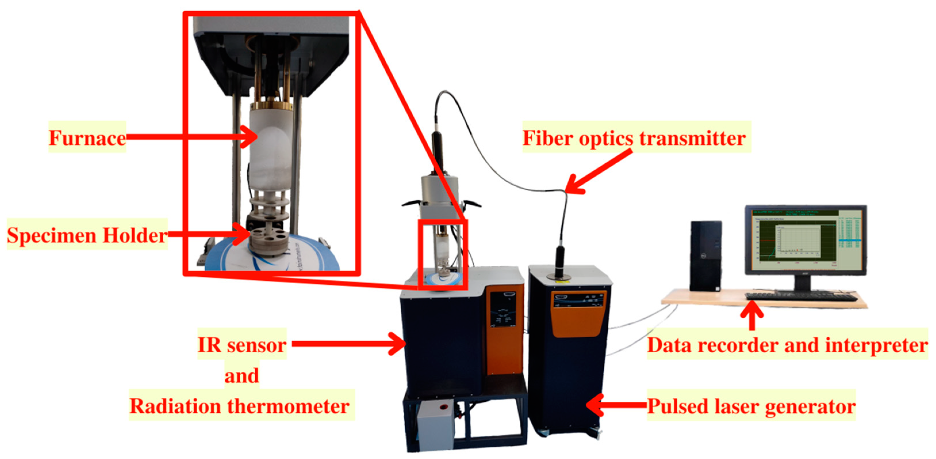
Figure 5.
LASER flash thermal analysis system.
Figure 5.
LASER flash thermal analysis system.
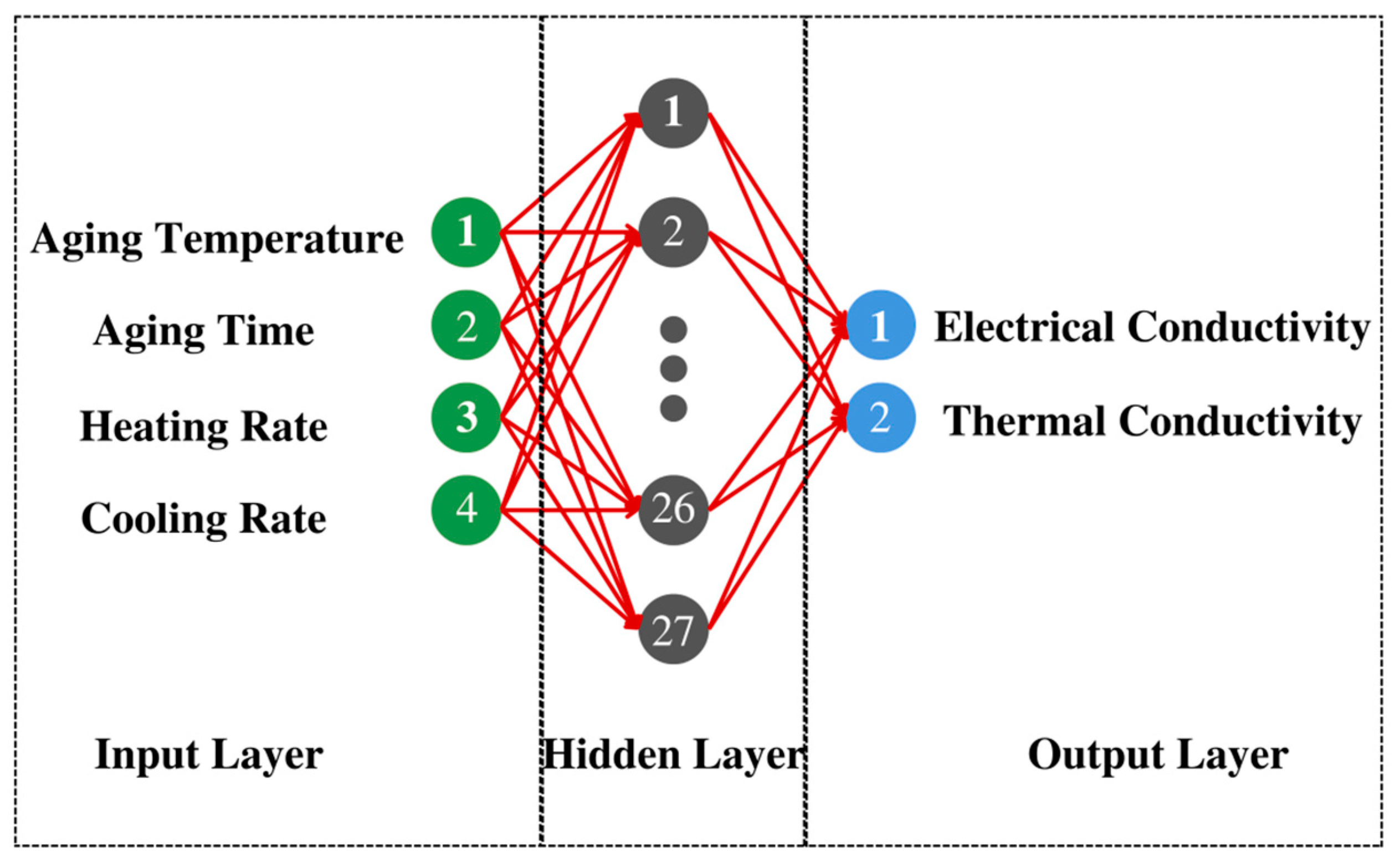
Figure 6.
Structure of Back Propagation Artificial Neural Network used in the study.
Figure 6.
Structure of Back Propagation Artificial Neural Network used in the study.
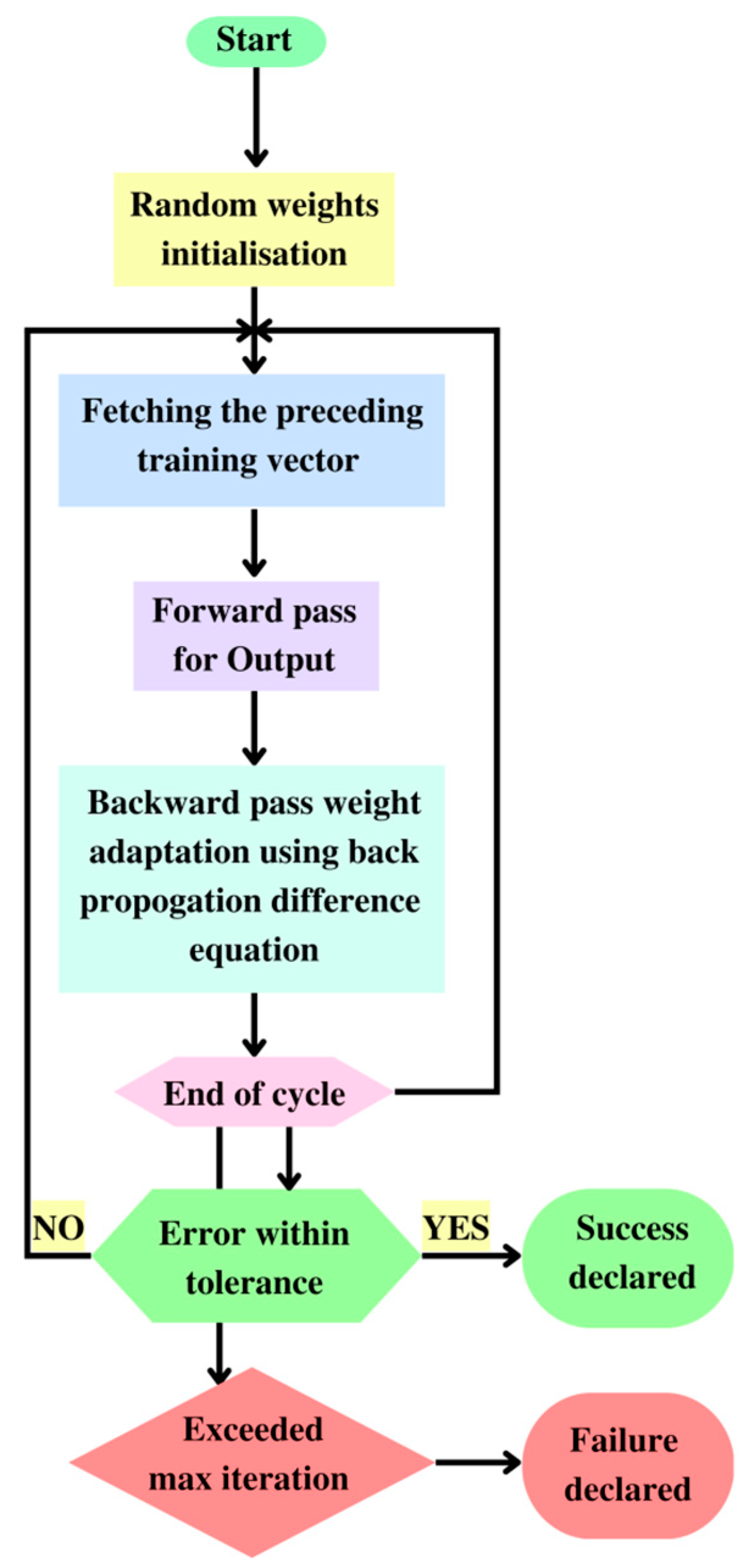
Figure 7.
Algorithm for the back-propagation artificial neural network program.
Figure 7.
Algorithm for the back-propagation artificial neural network program.
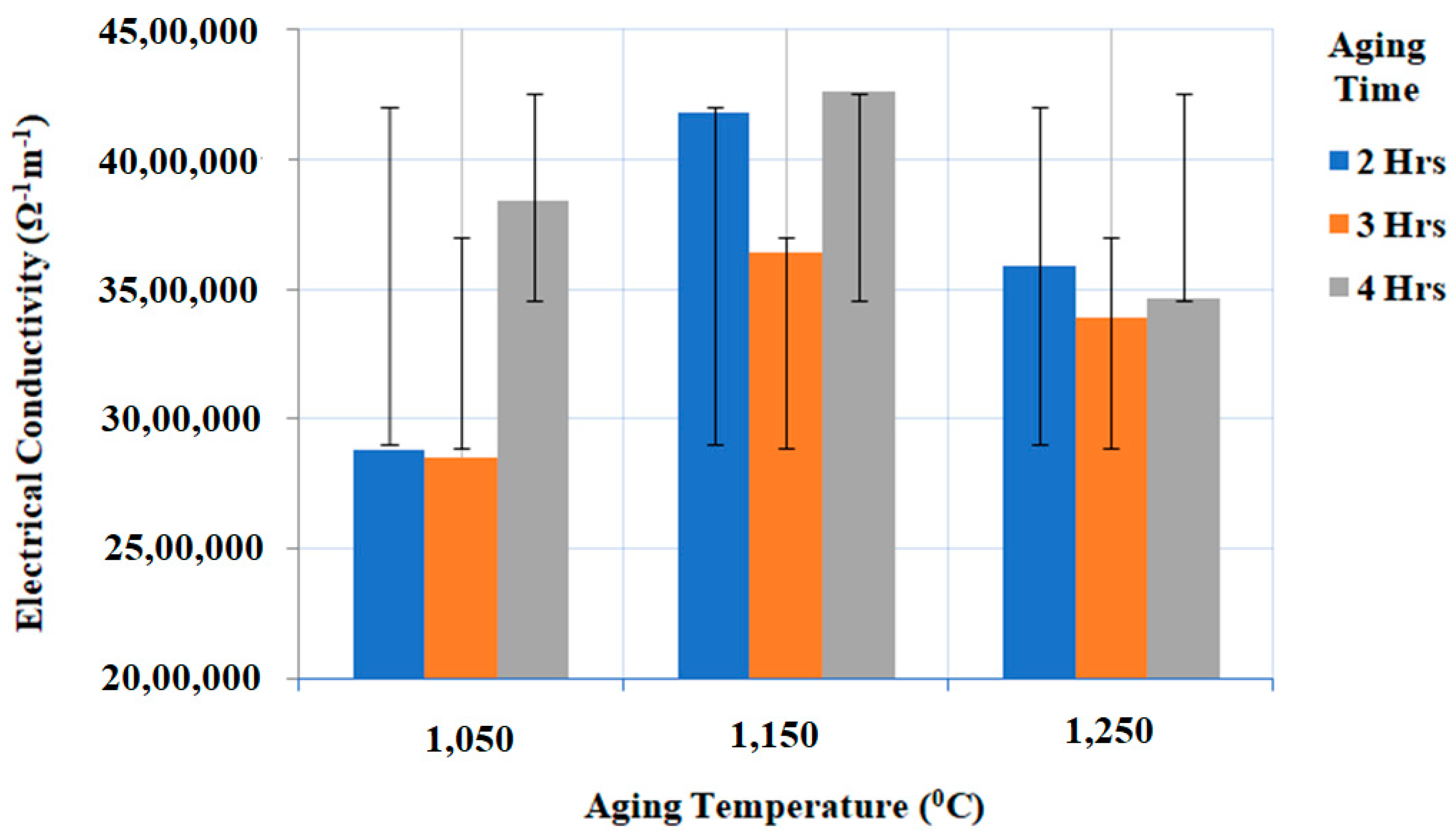
Figure 8.
Experimental results of electrical conductivity (Ω−1 m−1) under different aging temperatures (°C) and aging times (h) with the constant heating rate (°C/min), and cooling rate (°C/min).
Figure 8.
Experimental results of electrical conductivity (Ω−1 m−1) under different aging temperatures (°C) and aging times (h) with the constant heating rate (°C/min), and cooling rate (°C/min).
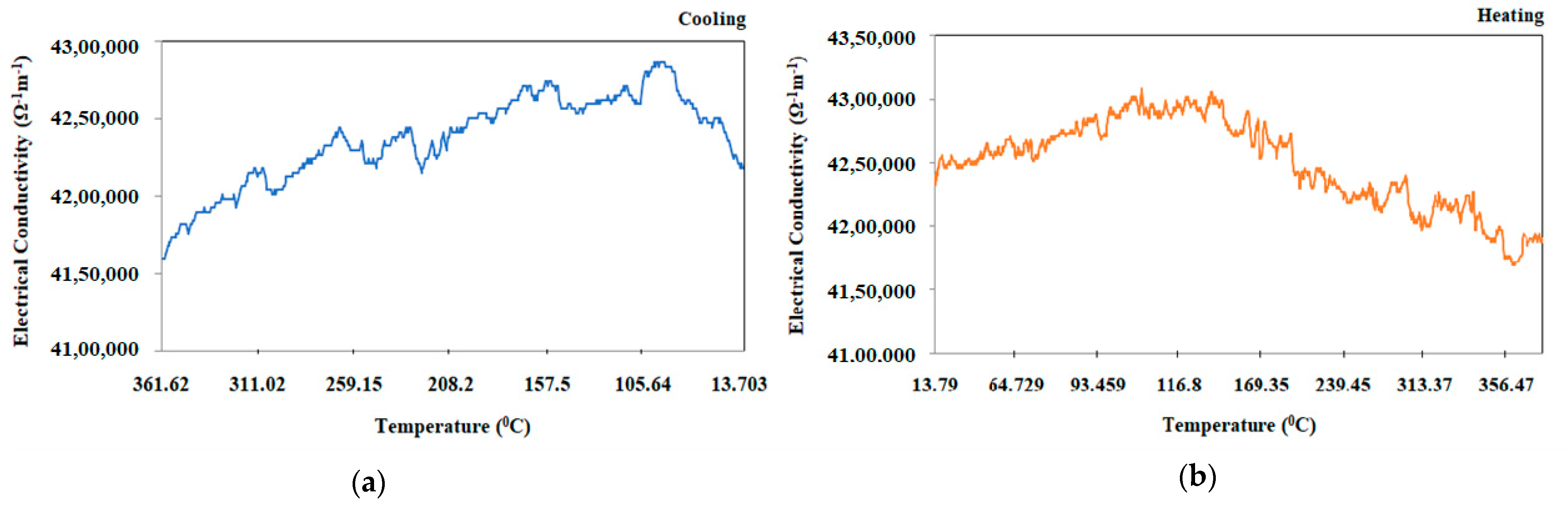
Figure 9.
Electrical conductivity versus temperature for Ti-6Al-4V-SiC (15 Wt.%) specimen processed at aging temperature (1150 °C), aging time (four hours), heating rate (25 °C/min), and cooling rate (5 °C/min) while cooling from 360–13 °C.
Figure 9.
Electrical conductivity versus temperature for Ti-6Al-4V-SiC (15 Wt.%) specimen processed at aging temperature (1150 °C), aging time (four hours), heating rate (25 °C/min), and cooling rate (5 °C/min) while cooling from 360–13 °C.
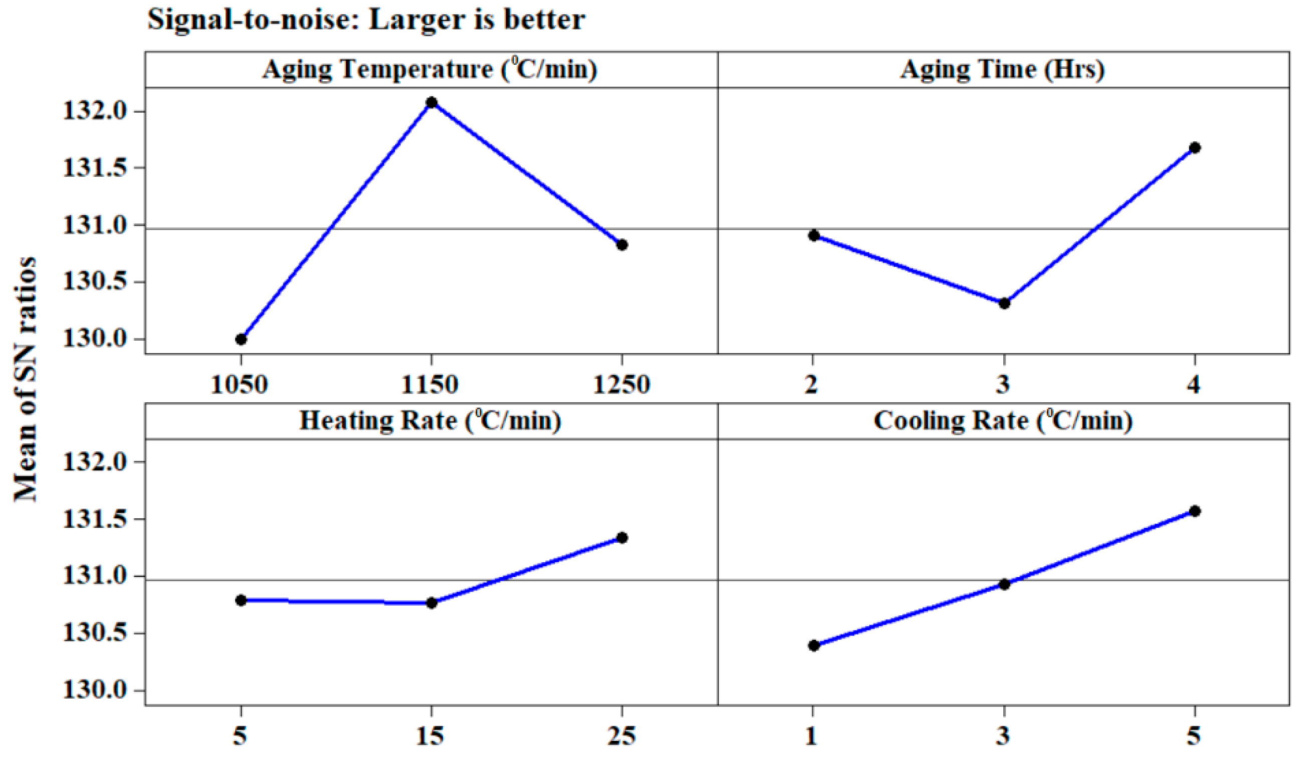
Figure 10.
Main effects plot for electrical conductivity (Ω−1 m−1).
Figure 10.
Main effects plot for electrical conductivity (Ω−1 m−1).
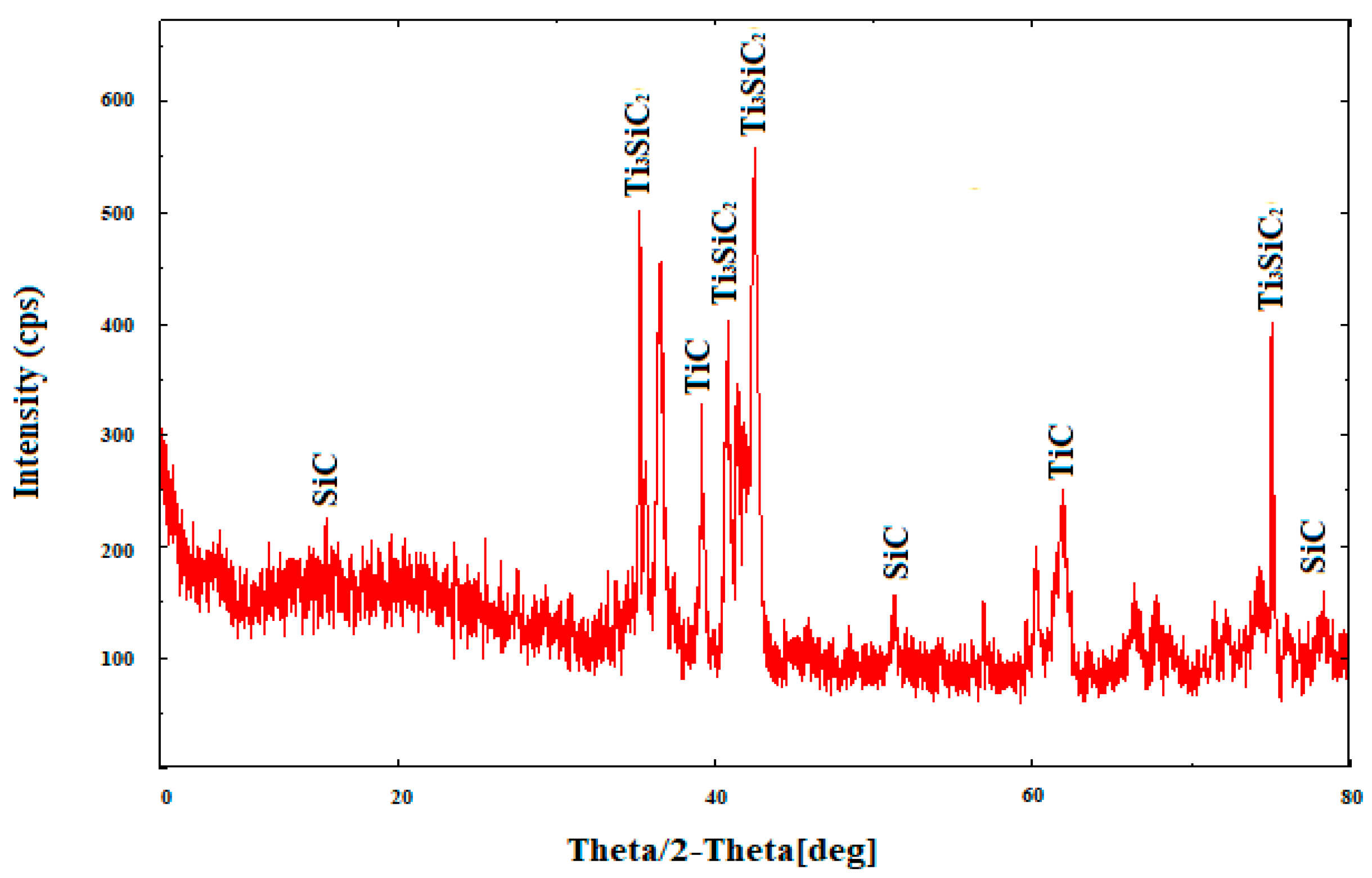
Figure 11.
XRD Peaks of Ti-6Al-4V-SiC(15 Wt.%) processed under aging temperature (1150 °C), aging time (four hours), heating rate (5 °C/min), and cooling rate (5 °C/min).
Figure 11.
XRD Peaks of Ti-6Al-4V-SiC(15 Wt.%) processed under aging temperature (1150 °C), aging time (four hours), heating rate (5 °C/min), and cooling rate (5 °C/min).
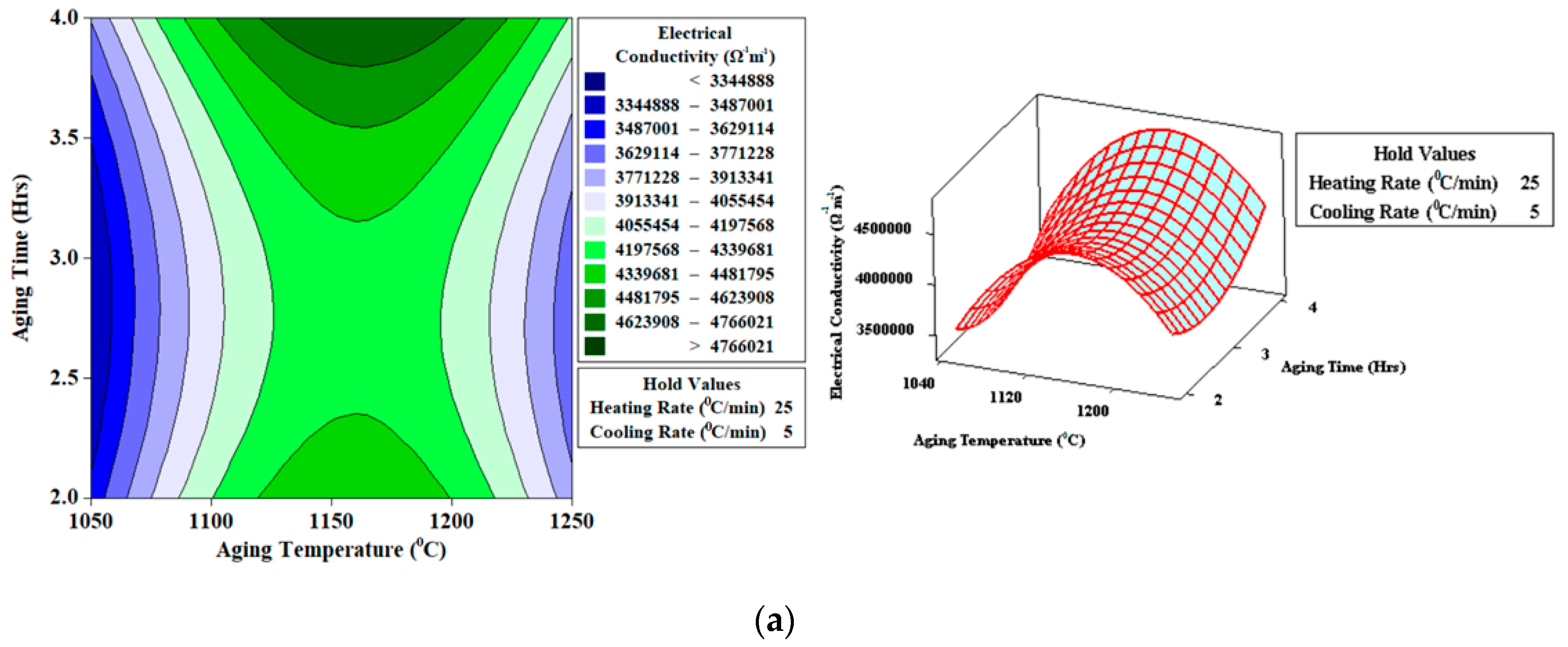
Figure 12.
Contour and surface plots for electrical conductivity (Ω−1 m−1) (a) Heating Rate (25 °C/min); Cooling Rate (5 °C/min) (b) Heating Rate (15 °C/min); Cooling Rate (3 °C/min) (c) Heating Rate (5 °C/min); Cooling Rate (1 °C/min).
Figure 12.
Contour and surface plots for electrical conductivity (Ω−1 m−1) (a) Heating Rate (25 °C/min); Cooling Rate (5 °C/min) (b) Heating Rate (15 °C/min); Cooling Rate (3 °C/min) (c) Heating Rate (5 °C/min); Cooling Rate (1 °C/min).
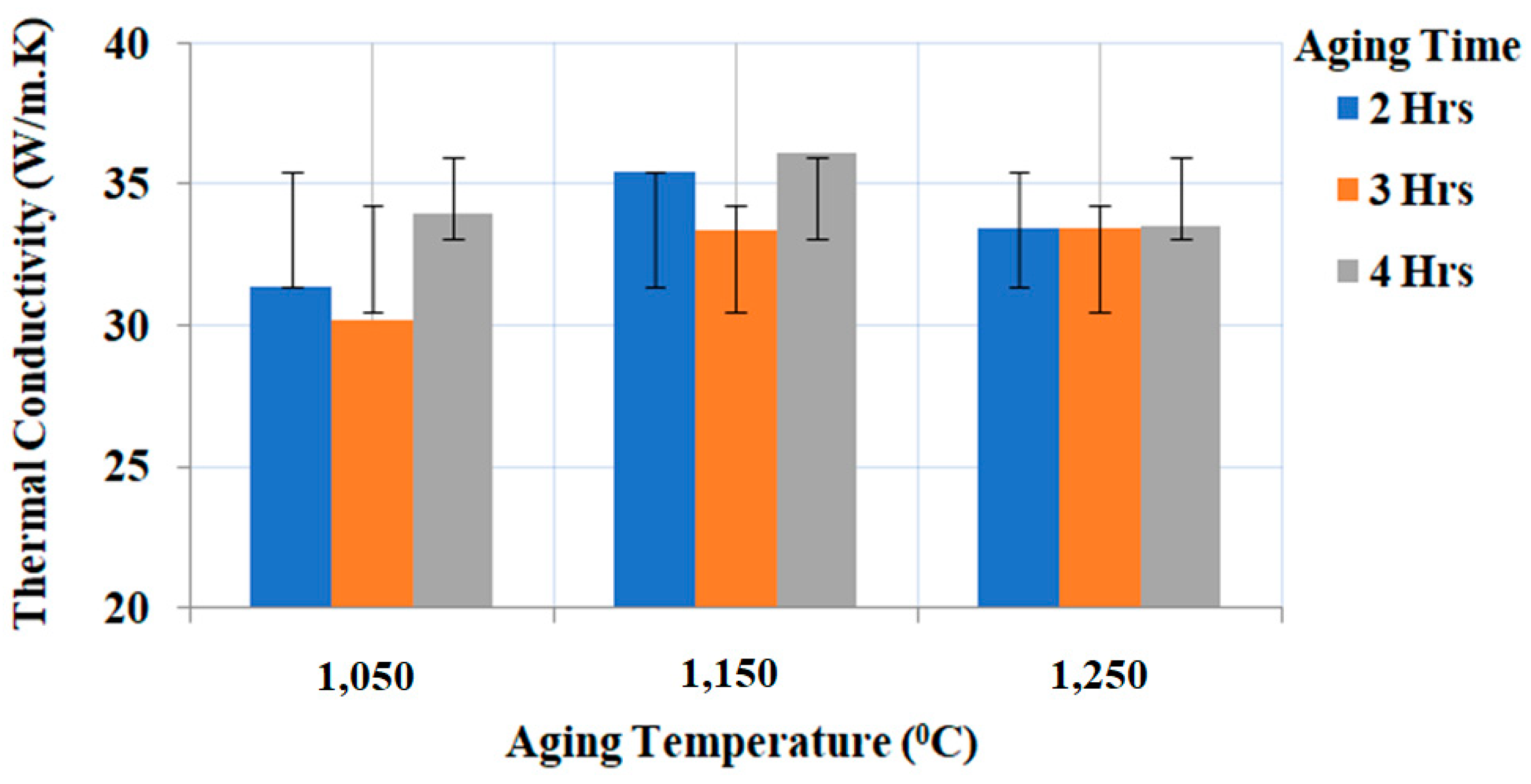
Figure 13.
Experimental results plot for thermal conductivity.
Figure 13.
Experimental results plot for thermal conductivity.
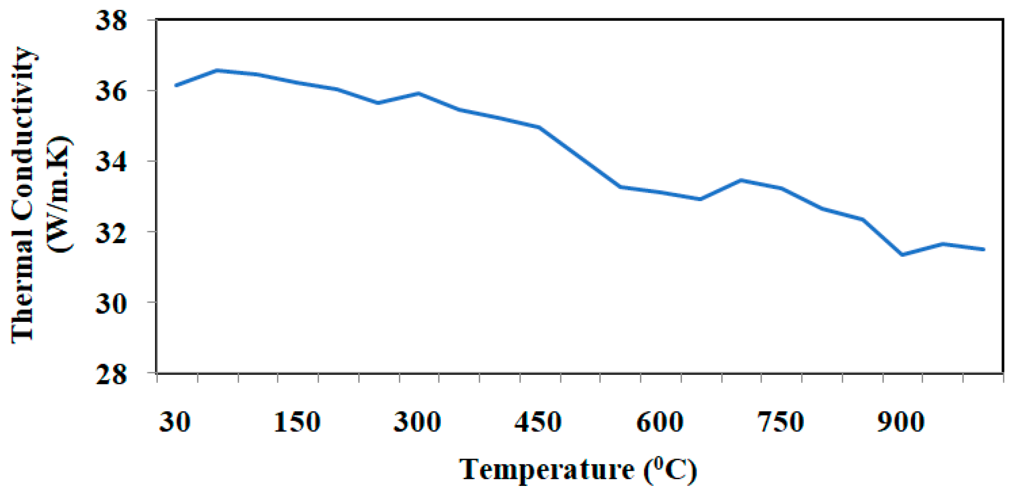
Figure 14.
Thermal conductivity versus temperature plot of Ti-6Al-4V-SiC(15 Wt.%) processed under aging temperature (1150 °C), aging time (four hours), heating rate (5 °C/min), and cooling rate (5 °C/min).
Figure 14.
Thermal conductivity versus temperature plot of Ti-6Al-4V-SiC(15 Wt.%) processed under aging temperature (1150 °C), aging time (four hours), heating rate (5 °C/min), and cooling rate (5 °C/min).
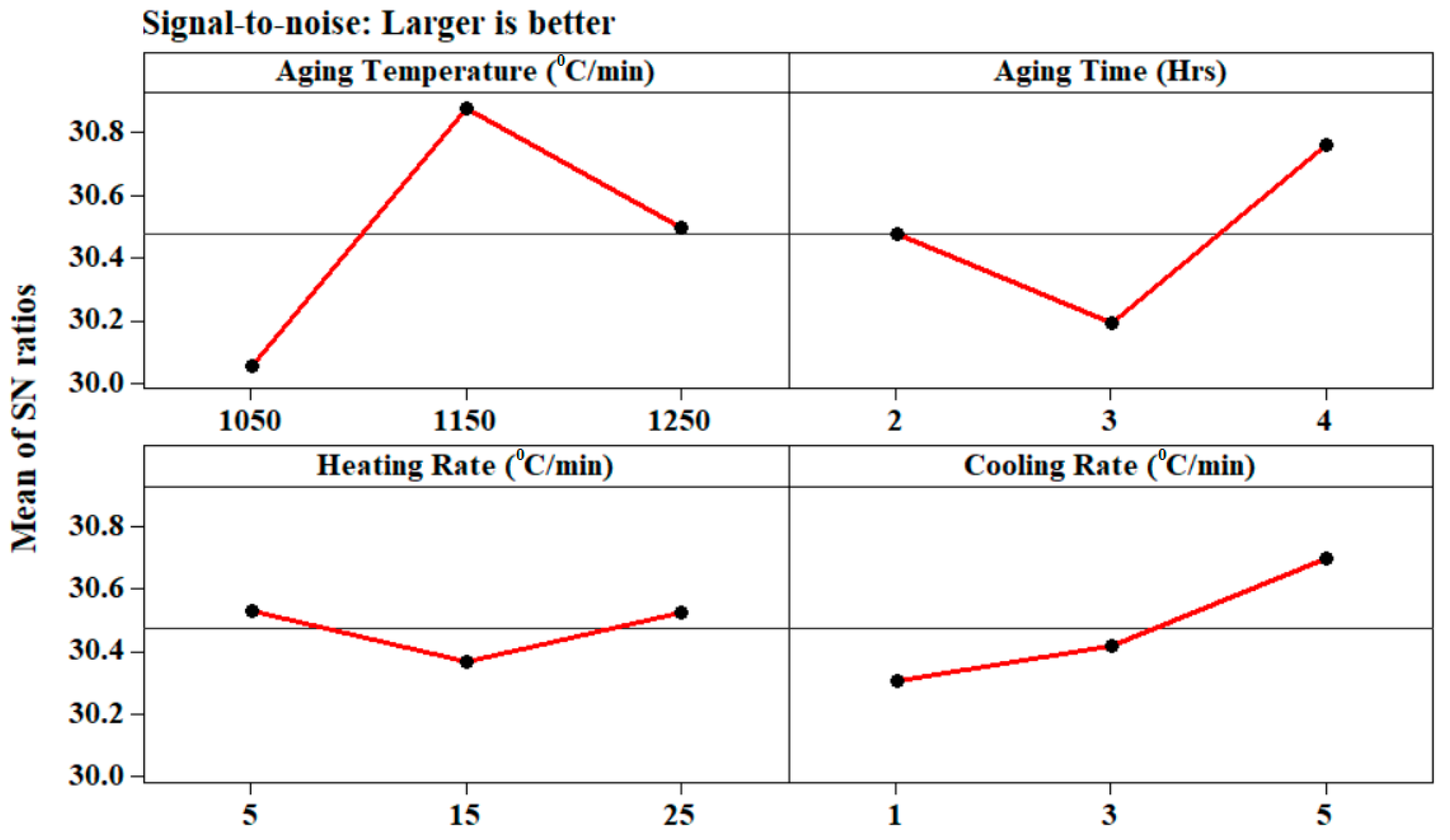
Figure 15.
Main effects plot for thermal conductivity.
Figure 15.
Main effects plot for thermal conductivity.
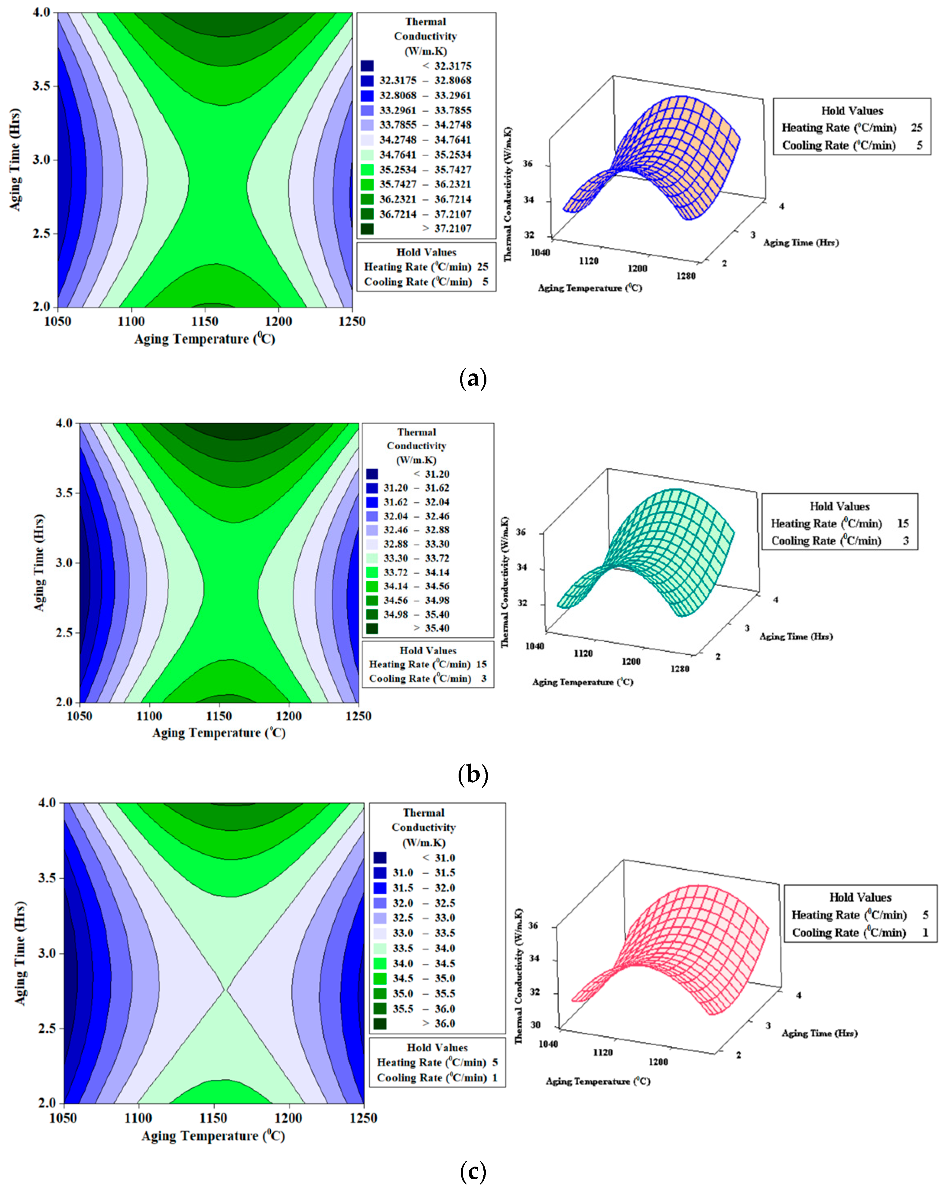
Figure 16.
Contour and surface plots for thermal conductivity (W/m·K) (a) Heating Rate (25 °C/min); Cooling Rate (5 °C/min) (b) Heating Rate (15 °C/min); Cooling Rate (3 °C/min) (c) Heating Rate (5 °C/min); Cooling Rate (1 °C/min).
Figure 16.
Contour and surface plots for thermal conductivity (W/m·K) (a) Heating Rate (25 °C/min); Cooling Rate (5 °C/min) (b) Heating Rate (15 °C/min); Cooling Rate (3 °C/min) (c) Heating Rate (5 °C/min); Cooling Rate (1 °C/min).
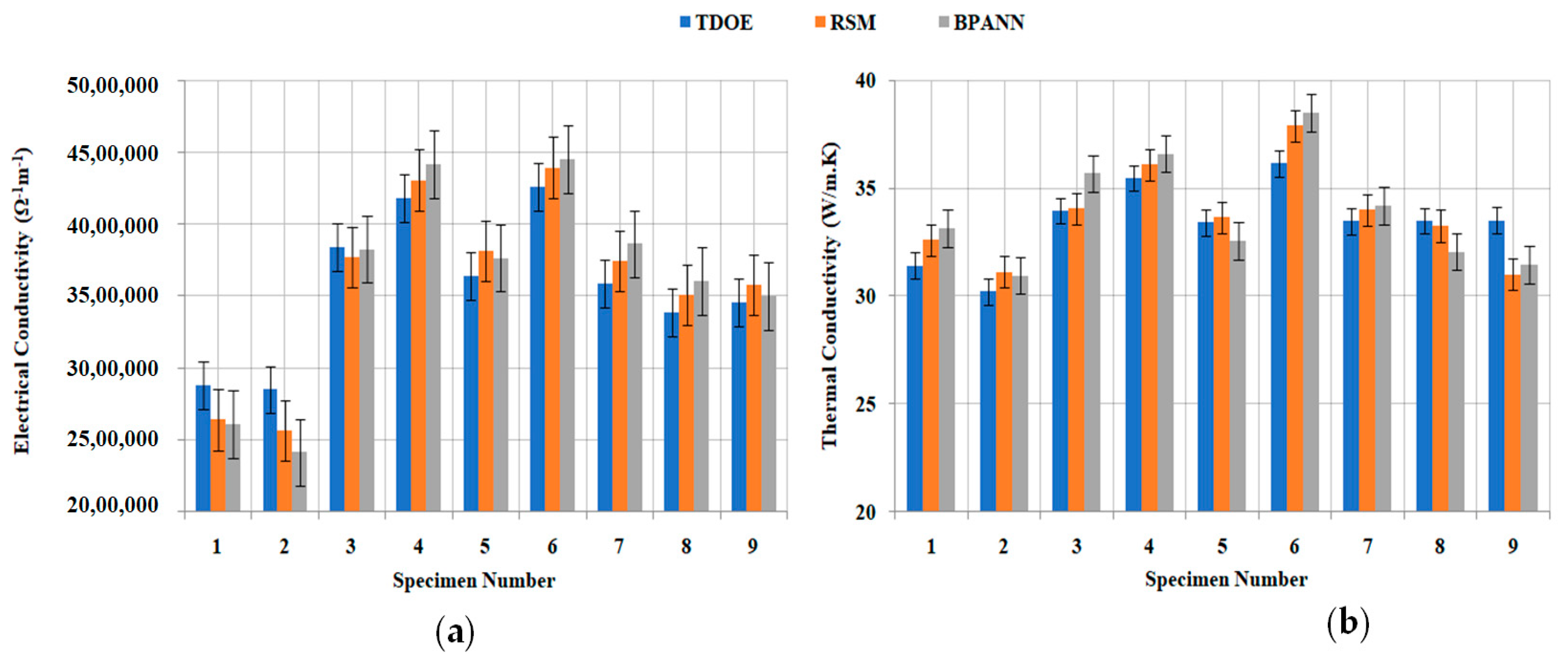
Figure 17.
Experimental versus RSM versus BPANN prediction values of (a) electrical conductivity and (b) thermal conductivity.
Figure 17.
Experimental versus RSM versus BPANN prediction values of (a) electrical conductivity and (b) thermal conductivity.
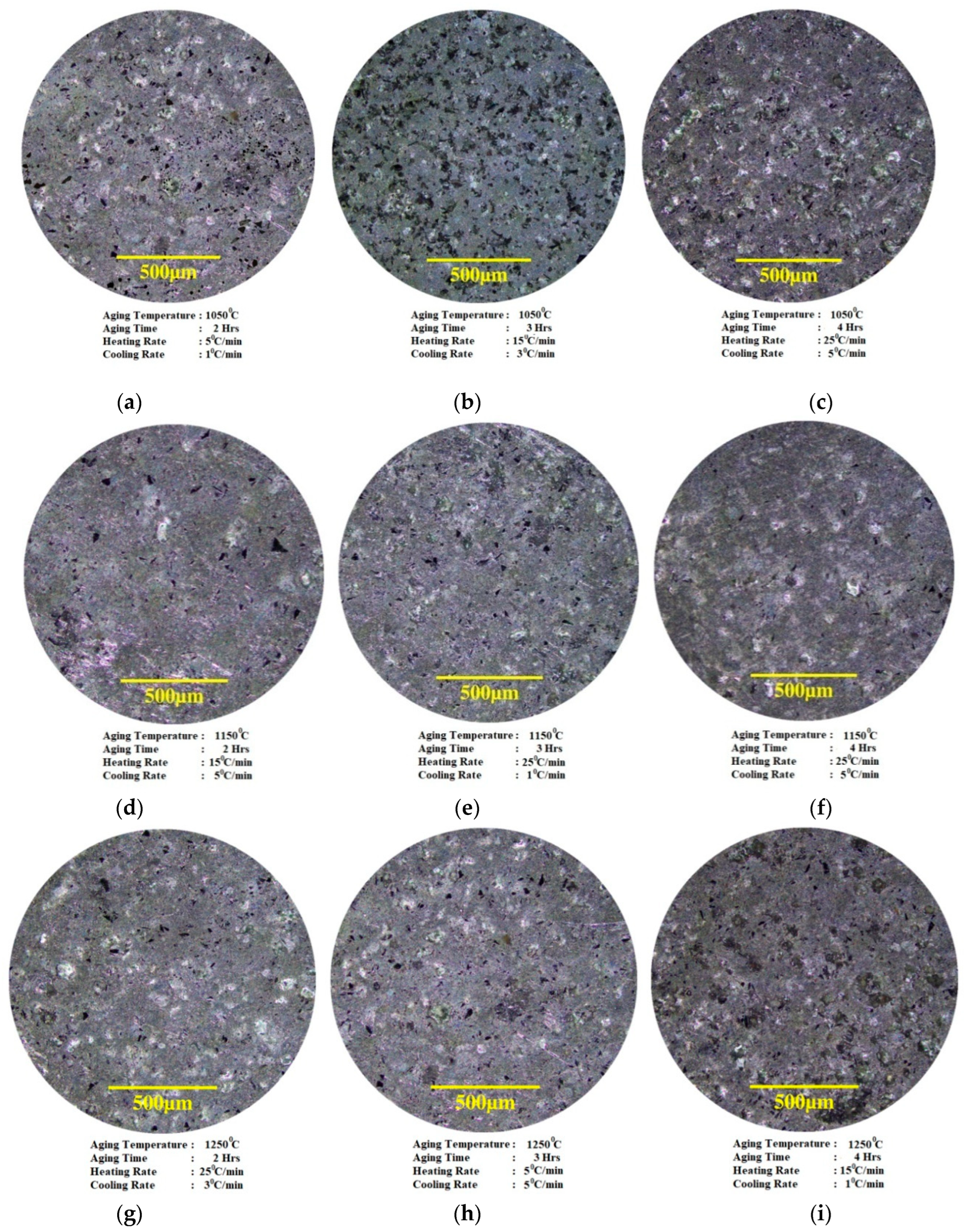
Figure 18.
Metallographic images of Ti-6Al-4V-SiC(15 Wt.%) processed under various conditions.
Figure 18.
Metallographic images of Ti-6Al-4V-SiC(15 Wt.%) processed under various conditions.
Figure 19.
Scanning Electron Microscope images of Ti-6Al-4V-SiC(15 Wt.%) processed under aging temperature (1150 °C), aging time (four hours), heating rate (25 °C/min), and cooling rate (5 °C/min).
Figure 19.
Scanning Electron Microscope images of Ti-6Al-4V-SiC(15 Wt.%) processed under aging temperature (1150 °C), aging time (four hours), heating rate (25 °C/min), and cooling rate (5 °C/min).
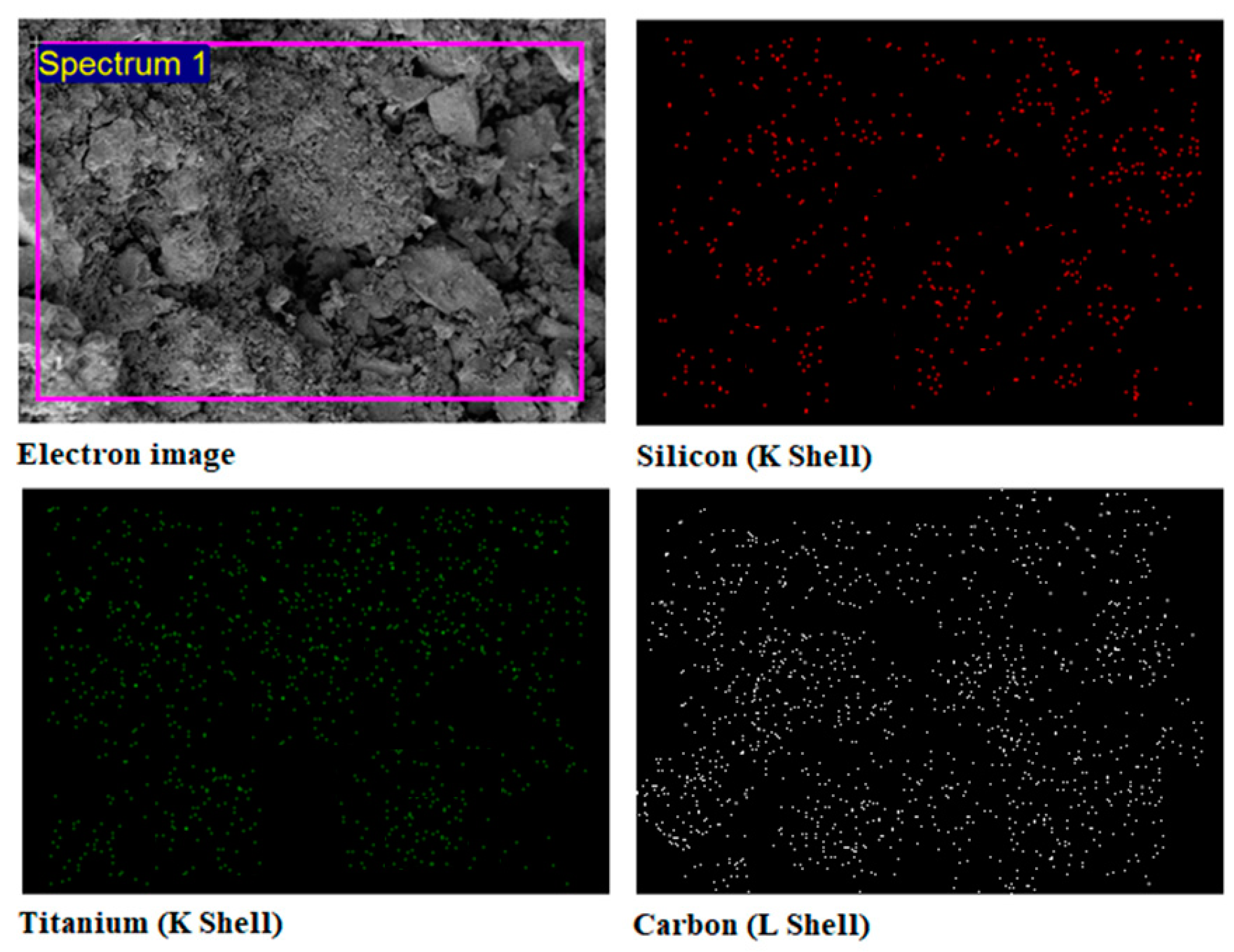
Figure 20.
Elemental Mapping of Ti-6Al-4V-SiC(15 Wt.%) composite processed under aging temperature (1150 °C), aging time (four hours), heating rate (25 °C/min), and cooling rate (5 °C/min) from electron dispersive X-ray analysis.
Figure 20.
Elemental Mapping of Ti-6Al-4V-SiC(15 Wt.%) composite processed under aging temperature (1150 °C), aging time (four hours), heating rate (25 °C/min), and cooling rate (5 °C/min) from electron dispersive X-ray analysis.
Table 1.
Composition (Wt%) of Ti-6Al-4V alloy [
20].
Table 1.
Composition (Wt%) of Ti-6Al-4V alloy [
20].
| Element | Aluminium | Vanadium | Iron | Oxygen | Carbon | Nitrogen | Titanium |
|---|
| Wt (%) | 6.1063 | 4.103 | 0.1675 | 0.1124 | 0.0235 | 0.0193 | Balance |
Table 2.
Composition (Wt%) of SiC reinforcement particle [
20].
Table 2.
Composition (Wt%) of SiC reinforcement particle [
20].
| Element | Carbon | Iron | Nitrogen | Aluminum | Calcium | Oxygen | Potassium | Silicon |
|---|
| Wt (%) | 1.172 | 0.664 | 1.4353 | 0.2557 | 0.1454 | 0.8642 | 0.3243 | Balance |
Table 3.
Thermal properties and Mechanical Properties of Ti-6Al-4V alloy [
20].
Table 3.
Thermal properties and Mechanical Properties of Ti-6Al-4V alloy [
20].
| Properties | Values (Units) |
|---|
| Density | 4.43 g/cm3 |
| Melting Point | 1604–1660 °C |
| Beta Transitional Temperature | 980 °C |
| Tensile Strength, Ultimate | 1170 Mpa |
| Tensile Strength, Yield | 1100 Mpa |
| Compressive Strength | 1070 Mpa |
| Modulus of Elasticity | 114 Gpa |
| Brinell Hardness | 379 BHN |
Table 4.
Thermal properties and Mechanical Properties of SiC [
20].
Table 4.
Thermal properties and Mechanical Properties of SiC [
20].
| Properties | Values (Units) |
|---|
| Density | 3.1 g/cm3 |
| Melting Point | 2730 °C |
| Beta Transitional Temperature | 2000 °C |
| Tensile Strength, Ultimate | 390 Mpa |
| Compressive Strength | 2000 Mpa |
| Modulus of Elasticity | 410 Gpa |
| Vicker’s Hardness | 2720 Hv |
Table 5.
Levels and Control factors for vacuum sintering (TDOE) [
20].
Table 5.
Levels and Control factors for vacuum sintering (TDOE) [
20].
| Control Factors | Levels |
|---|
| 1 | 2 | 3 |
|---|
| Aging Temperature (°C) | 1050 | 1150 | 1250 |
| Aging time (h) | 2 | 3 | 4 |
| Heating Rate (°C/min) | 5 | 15 | 25 |
| Cooling Rate (°C/min) | 1 | 3 | 5 |
Table 6.
L9 Orthogonal Array.
Table 6.
L9 Orthogonal Array.
| Trial No. | Factors and Levels |
|---|
| Aging Temp (°C) | Aging Time (h) | Heating Rate (°C/min) | Cooling Rate (°C/min) |
|---|
| 1 | 1 | 1 | 1 | 1 |
| 2 | 1 | 2 | 2 | 2 |
| 3 | 1 | 3 | 3 | 3 |
| 4 | 2 | 1 | 2 | 3 |
| 5 | 2 | 2 | 3 | 1 |
| 6 | 2 | 3 | 1 | 2 |
| 7 | 3 | 1 | 3 | 2 |
| 8 | 3 | 2 | 1 | 3 |
| 9 | 3 | 3 | 2 | 1 |
Table 7.
L31 Central Composite Design.
Table 7.
L31 Central Composite Design.
| Test No. | Blocks | A | B | C | D |
|---|
| 1 | 1 | −1 | −1 | −1 | −1 |
| 2 | 1 | 1 | −1 | −1 | −1 |
| 3 | 1 | −1 | 1 | −1 | −1 |
| 4 | 1 | 1 | 1 | −1 | −1 |
| 5 | 1 | −1 | −1 | 1 | −1 |
| 6 | 1 | 1 | −1 | 1 | −1 |
| 7 | 1 | −1 | 1 | 1 | −1 |
| 8 | 1 | 1 | 1 | 1 | −1 |
| 9 | 1 | −1 | −1 | −1 | 1 |
| 10 | 1 | 1 | −1 | −1 | 1 |
| 11 | 1 | −1 | 1 | −1 | 1 |
| 12 | 1 | 1 | 1 | −1 | 1 |
| 13 | 1 | −1 | −1 | 1 | 1 |
| 14 | 1 | 1 | −1 | 1 | 1 |
| 15 | 1 | −1 | 1 | 1 | 1 |
| 16 | 1 | 1 | 1 | 1 | 1 |
| 17 | 1 | −1 | 0 | 0 | 0 |
| 18 | 1 | 1 | 0 | 0 | 0 |
| 19 | 1 | 0 | −1 | 0 | 0 |
| 20 | 1 | 0 | 1 | 0 | 0 |
| 21 | 1 | 0 | 0 | −1 | 0 |
| 22 | 1 | 0 | 0 | 1 | 0 |
| 23 | 1 | 0 | 0 | 0 | −1 |
| 24 | 1 | 0 | 0 | 0 | 1 |
| 25 | 1 | 0 | 0 | 0 | 0 |
| 26 | 1 | 0 | 0 | 0 | 0 |
| 27 | 1 | 0 | 0 | 0 | 0 |
| 28 | 1 | 0 | 0 | 0 | 0 |
| 29 | 1 | 0 | 0 | 0 | 0 |
| 30 | 1 | 0 | 0 | 0 | 0 |
| 31 | 1 | 0 | 0 | 0 | 0 |
Table 8.
Control factors and levels for vacuum sintering (RSM).
Table 8.
Control factors and levels for vacuum sintering (RSM).
| Control Factors | Levels |
|---|
| −1 | +1 |
|---|
| Aging Temperature (°C) | 1050 | 1250 |
| Aging time (h) | 2 | 4 |
| Heating Rate (°C/min) | 5 | 25 |
| Cooling Rate (°C/min) | 1 | 5 |
Table 9.
Observations of the output response.
Table 9.
Observations of the output response.
| Itinerary | Description |
|---|
| Configuration of the network | 4-27-2 |
| Hidden Layer | 1 |
| Hidden neurons | 27 |
| Applied transfer function | “Logsig (sigmoid)” |
| Training pattern count | 9 |
| Testing pattern count | 9 |
| Epoch count | 8000 |
| (η) Factor for learning | 0.6 |
| (α) Factor of momentum | 1 |
Table 10.
Estimated Regression Coefficients for Electrical Conductivity (Ω−1 m−1).
Table 10.
Estimated Regression Coefficients for Electrical Conductivity (Ω−1 m−1).
| Term | Coef | SE Coef | T | P |
|---|
| Constant | 3,825,280 | 22,155 | 172.660 | 0.000 |
| A | 134,444 | 17,603 | 7.637 | 0.000 |
| B | 153,333 | 17,603 | 8.710 | 0.000 |
| C | 16,667 | 17,603 | 0.947 | 0.358 |
| D | 321,667 | 17,603 | 18.273 | 0.000 |
| A*A | −774,773 | 46,361 | −16.712 | 0.000 |
| B*B | 305,227 | 46,361 | 6.584 | 0.000 |
| C*C | 75,227 | 46,361 | 1.623 | 0.124 |
| D*D | 80,227 | 46,361 | 1.730 | 0.103 |
| A*B | 26,250 | 18,671 | 1.406 | 0.179 |
| A*C | −18,750 | 18,671 | −1.004 | 0.330 |
| A*D | 53,750 | 18,671 | 2.879 | 0.011 |
| B*C | −18,750 | 18,671 | −1.004 | 0.330 |
| B*D | 13,750 | 18,671 | 0.736 | 0.472 |
| C*D | −18,750 | 18,671 | −1.004 | 0.330 |
Table 11.
Analysis of variance for electrical conductivity.
Table 11.
Analysis of variance for electrical conductivity.
| Source | DF | Seq SS | Adj SS | Adj MS | F | P |
|---|
| Regression | 14 | 4.65159 × 10¹² | 4.65159 × 10¹² | 3.32257 × 10¹¹ | 59.57 | 0.000 |
| Residual Error | 16 | 89,244,311,111 | 89,244,311,111 | 5,577,769,444 | | 0.000 |
| Total | 30 | 4.74084 × 10¹² | | | | |
Table 12.
Estimated regression coefficients for thermal conductivity (W/m·K).
Table 12.
Estimated regression coefficients for thermal conductivity (W/m·K).
| Term | Coef | SE Coef | T | P |
|---|
| Constant | 33.8480 | 0.09255 | 365.719 | 0.000 |
| A | 0.4628 | 0.07354 | 6.293 | 0.000 |
| B | 0.5256 | 0.07354 | 7.147 | 0.000 |
| C | 0.0567 | 0.07354 | 0.771 | 0.452 |
| D | 0.8506 | 0.07354 | 11.566 | 0.000 |
| A*A | −2.5590 | 0.19367 | −13.213 | 0.000 |
| B*B | 1.3560 | 0.19367 | 7.002 | 0.000 |
| C*C | 0.1560 | 0.19367 | 0.805 | 0.432 |
| D*D | 0.5210 | 0.19367 | 2.690 | 0.016 |
| A*B | 0.2075 | 0.07800 | 2.660 | 0.017 |
| A*C | −0.0637 | 0.07800 | −0.817 | 0.426 |
| A*D | 0.0875 | 0.07800 | 1.122 | 0.278 |
| B*C | −0.0637 | 0.07800 | −0.817 | 0.426 |
| B*D | −0.0225 | 0.07800 | −0.288 | 0.777 |
| C*D | −0.0638 | 0.07800 | −0.817 | 0.426 |
Table 13.
Analysis of variance for thermal conductivity (W/m·K).
Table 13.
Analysis of variance for thermal conductivity (W/m·K).
| Source | DF | Seq SS | Adj SS | Adj MS | F | P |
|---|
| Regression | 14 | 41.822 | 41.8222 | 2.98730 | 30.69 | 0.000 |
| Residual Error | 16 | 1.5574 | 1.5574 | 0.09734 | | |
| Total | 30 | 43.3796 | | | | |
Table 14.
Electrical conductivity and thermal conductivity of Ti-6Al-4V-SiC(15 Wt.%) specimen processed under various processing conditions.
Table 14.
Electrical conductivity and thermal conductivity of Ti-6Al-4V-SiC(15 Wt.%) specimen processed under various processing conditions.
| Trial No. | Electrical Conductivity (Ω−1 m−1) | Error (%) | Thermal Conductivity (W/m·K) | Error (%) |
|---|
| TDOE | RSM | BPANN | RSM | BPANN | TDOE | RSM | BPANN | RSM | BPANN |
|---|
| 1 | 2,880,000 | 2,641,592 | 2,611,491 | 9.025 | 1.152 | 31.41 | 32.59844 | 33.1425 | 3.645 | 1.641 |
| 2 | 2,850,000 | 2,567,891 | 2,415,789 | 10.98 | 6.296 | 30.22 | 31.11954 | 30.95 | 2.89 | 0.547 |
| 3 | 3,840,000 | 3,769,585 | 3,825,495 | 1.867 | 1.461 | 33.95 | 34.05957 | 35.6830 | 0.321 | 4.549 |
| 4 | 4,180,000 | 4,305,898 | 4,413,895 | 2.923 | 2.446 | 35.46 | 36.07785 | 36.5815 | 1.712 | 1.376 |
| 5 | 3,640,000 | 3,812,258 | 3,764,822 | 4.518 | 1.259 | 33.41 | 33.64925 | 32.5512 | 0.711 | 3.373 |
| 6 | 4,260,000 | 4,393,699 | 4,452,174 | 3.042 | 1.313 | 36.15 | 37.88915 | 38.4951 | 4.59 | 1.574 |
| 7 | 3,590,000 | 3,745,102 | 3,862,733 | 4.141 | 3.045 | 33.46 | 33.99454 | 34.1920 | 1.572 | 0.577 |
| 8 | 3,390,000 | 3,508,955 | 3,605,897 | 3.390 | 2.688 | 33.49 | 33.24958 | 32.0552 | 0.723 | 3.726 |
| 9 | 3,460,000 | 3,577,488 | 3,498,621 | 3.284 | 2.254 | 33.51 | 31.01259 | 31.4586 | 8.052 | 1.417 |


 ,
, 


