

A Comparison between the Results from Linear Analysis and Nonlinear Analysis in the Context of Simulation of Biological Materials

Department of Mechanical and Industrial Engineering, Manipal Institute of Technology, Manipal Academy of Higher Education, Manipal 576104, Karnataka, India
J. Compos. Sci. 2023, 7(3), 109; https://doi.org/10.3390/jcs7030109
Submission received: 21 September 2022
/
Revised: 15 November 2022
/
Accepted: 3 January 2023
/
Published: 8 March 2023
(This article belongs to the Special Issue Advanced Polymeric Composites and Hybrid Materials)
Abstract
:Surgical simulations require fast and accurate simulation of biological materials. In general, linear analysis is faster but less accurate, whereas nonlinear analysis is more accurate but slower. In this work, a kidney is simulated by using both linear analysis and nonlinear analysis, the results are compared, and the errors quantified. The software package ANSYS is used for the purpose. This work presents detailed results and comparison of linear and nonlinear analysis in the context of simulation of a human kidney, which is not easily found in the literature. The results reinforce the idea that linear analysis is a useful tool for simulating biological materials when solution time is as much important as the accuracy of solutions.
1. Introduction
Surgeons need to develop certain skills like eye-hand coordination for successfully carrying out certain surgical procedures [1,2]. The skills they need to acquire may vary from one surgical procedure to another. Traditionally, surgeons were trained using real patients. Since it is risky to allow an inexperienced surgeon to operate on real patients, there is a need to develop simulators that can simulate different surgical procedures. A few simulators are already available in the market [3,4,5,6,7,8,9], and more are being developed. The surgical simulators that are already available in the market have been found to be simulating a few surgical procedures, with varying levels of fidelity.
Surgical simulators should be able to simulate the mechanical behaviour of biological materials. In fact, fidelity of a surgical simulator largely depends on how realistically the mechanical behaviour of biological materials (organs) is incorporated into the simulator.
Mainly two approaches are being used to incorporate the mechanical behaviour of biological materials into surgical simulators. They are: using spring-mass models, and using continuum-mechanics based models. Spring-mass models are generally faster but less accurate whereas continuum-mechanics based models are slower but more accurate. Fidelity of a surgical simulator depends on both the speed and the accuracy of simulations. Since modern computers are faster, they can simulate even the continuum mechanics-based models reasonably fast. Hence it is generally agreed that the approach of using continuum-mechanics based models is preferable over the approach of using spring-mass models.
A few continuum-mechanics based models that are available are: using the finite element method, using the boundary element method, using meshfree methods. The finite element method is the most popular and the most well-established continuum-mechanics based method. Hence finite element method is utilized in the present work. Biological materials are inherently nonlinear, and the finite element method is suitable for simulating both linear and nonlinear materials.
It is a well-known fact that the nonlinear simulation gives more accurate results when compared to the linear simulation, if the mechanical behaviour is nonlinear. It is also a well-known fact that the nonlinear analysis (simulation) takes more time when compared to the linear analysis (simulation). As already mentioned earlier, fidelity of a surgical simulator largely depends on the level of realism offered by the simulations, and the realism offered by the simulations depend both on the speed and the accuracy of simulations. Hence there is a need to further investigate whether a linear analysis or a nonlinear analysis is preferable to be employed in the simulations, when building a particular surgical simulator when the underlying material behaviour (mechanical behaviour) is nonlinear, and the underlying mechanical behaviour most of the time is nonlinear in the case of surgical simulators. Hence, one cannot just concentrate only on speed or accuracy, but one needs to concentrate on both speed and accuracy. This means that one cannot just decide to use only the nonlinear analysis or only the linear analysis while building every simulator; one needs to carry out further studies, by carrying out both the linear analysis and the nonlinear analysis, to decide which of the two simulations (analyses) is more suitable for a particular purpose.
To sum it up, simulation of biological materials assumes significance in the context of surgical simulations [10,11,12,13,14,15,16,17,18,19,20]. Biological materials are inherently nonlinear. Relevant literature indicates that it is preferable to use continuum–mechanics-based computational techniques (e.g., finite element method, boundary element method) for the simulation of biological materials. Continuum–mechanics-based simulation of biological materials may, at times, consider biological materials to be approximated as linear elastic materials, e.g., [21]. Although nonlinear analysis may result in more accurate simulations, assuming biological materials to be linearly elastic in such cases results in faster simulations without significantly affecting accuracy.
Hence both linear and nonlinear analyses have their own importance in the context of simulation of biological materials. Although linear analysis in general gives less accurate results when compared to nonlinear analysis, in some cases, linear analysis can offer better realism because it is faster. Hence, in the context of simulation of biological organs, there is a need to compare the realism offered by linear analysis with that offered by nonlinear analysis, on a case-by-case basis. Studies that offer detailed side-by-side comparison of results from linear simulation and nonlinear simulation are rare to find in the literature. Hence in this paper, detailed quantitative results from both linear and nonlinear analyses are presented in the form of figures and tables, in the context of real-time simulation of a human kidney. The results presented in this paper could be useful when building a surgical simulator that can simulate palpation of kidney.
This paper simulates a human kidney, a biological organ, by using the finite element method. Detailed results are presented by using linear analysis and also by using nonlinear analysis. Percentage error resulting from the use of linear elastic analysis (when compared to nonlinear analysis) is also calculated.
The analyses presented in this paper are not specific to any particular renal surgery. Kidney is considered homogeneous and isotropic.
2. Materials and Methods
In this paper, a comparison is made between the results obtained by using linear elastostatic analysis and geometrically nonlinear analysis. The commercial software package ANSYS is used for the purpose; ANSYS is used for both linear and nonlinear analysis.
The biological organ simulated in this paper was the left kidney of the Visible Human male [22]. The kidney was extracted from CT scan images that are downloadable from the Visible Human Project [22] for free. The images used were that of a human male (Visible Human male). The author followed the procedure explained in [23] to obtain the 3D model (geometry) of the human kidney. The procedure involved segmentation, 3D reconstruction etc., as explained in [23]. The next few paragraphs give some more details about the way the 3D model of the kidney (geometry) was obtained.
Visible Human Project (VHP) provides freely downloadable images of cross-sections of a complete male human body and a complete female human body. The images were obtained by slicing a male cadaver (known as Visible Human male) and a female cadaver (known as Visible Human female). The images are available as CT or MRI images. All the images related to the male cadaver are together called as Visible Man data set, and all the images related to the female cadaver are together called as Visible Woman data set. The Visible Man data set and the Visible Woman data set are collectively called as the Visible Human Data Set (VHD). The Visible Man data set is of size 15 gigabytes, and the Visible Woman data set is of size 40 gigabytes. A license that was free of cost was required for downloading the images earlier, but no license is required now. As mentioned earlier, CT scan images from Visible Man data set are used in the present work. In the case of Visible Man data set, to get the CT scan images, axial scans of the entire male cadaver were carried out at an interval of 1 mm, and there are 1871 CT scan images in total. CT scan images for the Visible Man data set have a resolution of 512 by 512 pixels, and 12 bits of gray tone for each pixel. The geometry that is used for the simulations in the present work, i.e., left kidney of Visible Human male is extracted from the Visible Man data set by using the free software packages ImageJ, ITK-SNAP, and MeshLab, and the commercial software package Rhinoceros, by following the procedure given by [23]. The exact procedure that was followed to get the 3D model of the left kidney of the Visible Human male is explained in the next few paragraphs in some detail, and the explanations closely match the explanations provided in [23].
The Visible Human Project provides images in different file formats. Present work uses images in the ‘png’ format since this is the file format recommended by VHP. The reason for using the CT scan images (instead of MRI images) is that the file size of CT-scan images is small, and the images are good enough for reconstructing a 3D model of the whole kidney (i.e., inner (or finer) details of kidney are not present; reconstructed 3D model represents just the outer surface of kidney). Also, one can easily identify human kidney in the CT-scan images of VHD. In the present work, the free and open-source software package ImageJ is used to form an image stack which contains the kidney. ITK-SNAP, another free and open-source software package, is used for segmentation and 3D reconstruction to the correct scale. MeshLab, one more free and open-source software package, is used to control the level of detail in the reconstructed 3D model; it also serves as a tool to smoothen the 3D model and reduce its file size. Now the method of using these three software packages (ImageJ, ITK-SNAP, and MeshLab) is explained in some detail.
ImageJ [24,25] was used to form a stack of images that belong to the kidney. From the CT scan images (png format) from the Visible Man data set, the images which belong to left kidney were to be identified. Upon viewing individual images in ImageJ, one could conclude that for visible human male, the left kidney is contained between the images ‘cvm1551f.png’ and ‘cvm1692f.png’ (47 images in total). These 47 images were copied into an empty folder. Now, to form an image stack, the menu item ‘File -> Import -> Image Sequence…’ was selected, browsed to the location of the folder containing 47 images and the first image in the folder was selected and the prompts were followed (with default options); all 47 images were now displayed in ImageJ as an image stack; now, the menu item ‘File -> Save As -> Raw Data…’ was selected to save the image stack in the ‘*.raw’ format (where * is the file name given).
ITK-SNAP [26] was used next to perform segmentation and 3D reconstruction. ITK-SNAP does the segmentation and 3D reconstruction to the correct scale. Hence header information for the images in the image stack is essential. VHD contains header information for each of the images in its database. Upon going through the header files of each of the 47 images of male, one can note that the following header information is identical for all the 47 images: Image matrix size—X = 512, Image matrix size—Y = 512, Image dimension—X = 460 mm, Image dimension—Y = 460 mm, Image pixel size—X = 0.898438, Image pixel size—Y = 0.898438, Screen Format = 16 bit, Spacing between scans = 3 mm. Next, the menu item ‘File -> Open Greyscale Image…’ was selected, browsed to the location of the image stack for male, the prompts were followed and the header information was supplied. The ‘missing header information’ to be supplied for the image stack was: Image dimensions: X: 512, Y: 512, Z: 47, Voxel spacing: X = 0.898438, Y = 0.898438, Z = 3, Voxel representation: 16 bit, unsigned. Once the header information was supplied, image stack was displayed in ITK-SNAP. One could browse through all the 47 images in the image stack. Now the task was to do the segmentation. The ‘Polygon tool’ from the ‘IRIS Toolbox’ was selected, for slice-by-slice manual segmentation. The ‘continuous’ radio button under ‘Polygon Tool’ was selected. The mouse was clicked and the mouse cursor was dragged along the edge of the kidney (as seen in the axial view (window)), carefully. This drew the contour of the edge of the kidney. Now, right clicked on the image, and the ‘accept’ button was selected to create the segmentation for the image on display. This process was to be repeated for all images in the image stack, which contain pixels that belong to the left kidney. Once the segmentation was over, 3D reconstruction was to be carried out. This was accomplished by the menu item ‘Segmentation -> Save As Mesh…’, following prompts, browsing to the location where the reconstructed model was to be stored, and giving a name in the format ‘path\*.stl’ for the file that represented the reconstructed 3D model (where ‘path’ is the complete path, e.g., C:\Users\PC\Desktop\*.stl, and * is any file name). Now, a 3D reconstruction of the left kidney for the visible human male was over.
MeshLab [27] was used next to reduce the total number of faces describing the 3D model of the kidney. This step was required because the 3D surface model of the kidney obtained through the use of ITK-SNAP was of very large size and was described by a very large number of surface triangles. MeshLab was helpful in reducing the total number of surface triangles that were needed to describe the 3D surface model satisfactorily. It also served as a tool to smoothen the reconstructed 3D geometry; after using smoothing features provided by MeshLab, it was necessary to scale the 3D model to the correct dimensions, to strictly retain the original dimensions. MeshLab could also improve the triangle quality of surface triangles of the 3D surface model. It could also reduce the file size.
The geometry of kidney obtained by using the procedure explained above was not a 3D solid model; it was a 3D surface model made up of 3D surface triangles. Since ANSYS was to be used next for the linear and nonlinear simulations on the liver, a 3D solid model of the liver was required. This was because a 3D surface model cannot be imported into ANSYS whereas a 3D solid model can readily be imported into ANSYS for further analyses (simulations). Hence the 3D surface model of the kidney (obtained above) was converted into a 3D solid model by using the commercial software package Rhinoceros [28]. Now the geometry (geometry of liver) required for the linear and nonlinear simulations (analyses) was ready.
The material properties used were [29] the following: Young’s modulus = 150 N/mm2, Poisson’s ratio = 0.4, and only geometric nonlinearity was considered (the material was considered to be linearly elastic, but the material could undergo large deformation). The selection of this material model was justified by the fact that it was much more important to incorporate geometric nonlinearity when compared to incorporating nonlinear material models, and many a time just incorporating geometric nonlinearity, while using just the linear elastic constitutive model, results in highly accurate simulations [30].
Human kidneys are subjected to boundary conditions that are so complicated that it is virtually impossible to reproduce the boundary conditions in a computer model. Hence the kidney was subjected to arbitrary boundary conditions here. The idea was that if a computer model could give accurate solutions for many sets of arbitrary boundary conditions, then it was reasonable to assume that the user could specify whatever set of boundary conditions the user wanted to impose and the solution obtained for the specified set of boundary conditions would be accurate. The kidney considered in this work was subjected to three different sets of arbitrary boundary conditions, giving rise to three different problems to be solved. These three problems were named as Problem 1, Problem 2, and Problem 3.
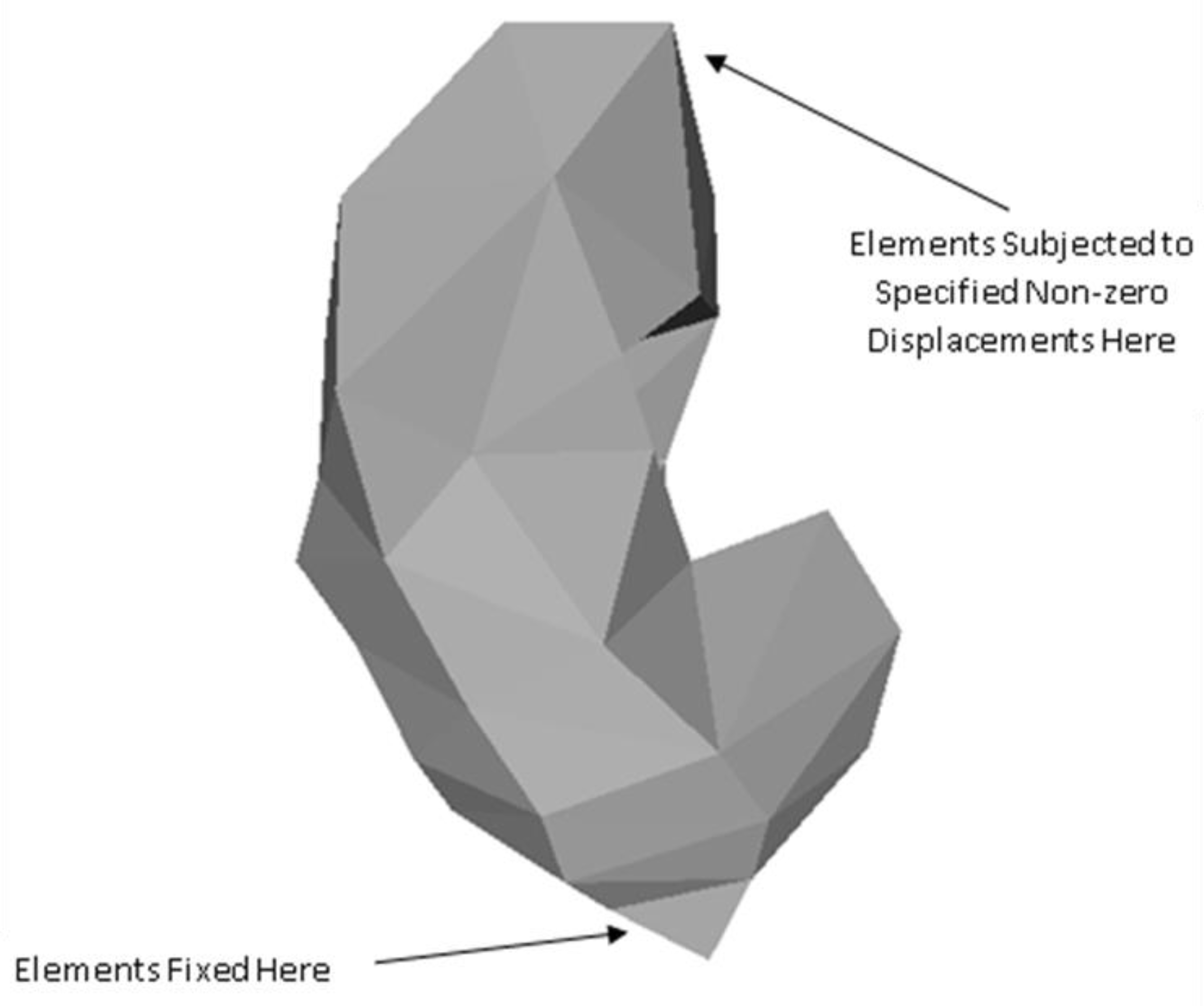
Geometry and material properties were the same for Problem 1, Problem 2, and Problem 3. With regard to boundary conditions, for each of Problem 1, Problem 2, and Problem 3, some portion of the surface of the kidney was assumed to be fixed while a known displacement was assumed to be applied on the surface of the kidney at some other location. The location where the kidney was assumed to be fixed, and the location where a known displacement was applied were the same for Problem 1, Problem 2, and Problem 3. Hence the only difference between Problem 1, Problem 2, and Problem 3 was that the directions of the applied nonzero displacements were different. The location where the kidney was fixed (i.e., zero displacement specified in all the x, y, and z directions), and the location where a specified non-zero displacement was specified are shown in Figure 1. As mentioned earlier, these locations were the same for Problem 1, Problem 2, and Problem 3.
The geometry of the kidney was discretized into 3D elements using the software package ANSYS. The element type used was Tet 10node 187. The geometry was discretized into 782 nodes in total. The element numbers for the elements at the location where the kidney was fixed were observed to be 8, 15, and 24. These elements were fixed, i.e., subjected to the zero-displacement boundary condition in each of the x, y, and z directions. The element number 94 happened to be the element located at the location where the known nonzero displacements were applied.
The difference between Problem 1, Problem 2, and Problem 3, was that, for Problem 1, the element 94 was subjected to the non-zero displacement of 5 mm in the x direction. For Problem 2, the element 94 was subjected to the non-zero displacement of 5 mm in the y direction. For Problem 3, the element 94 was subjected to the non-zero displacement of 5 mm in the z direction. The value of 5 mm was chosen for all the problems because this value of displacement corresponded to about 5% deformation along the largest dimension of the biological organ considered, if the load that caused the deformation was applied along the same direction. Of course, specifying 5 mm displacement in other directions could result in deformations that were not close to the 5% deformation. However, one could note that the idea here was to specify physically meaningful non-zero displacement boundary conditions. This author had not aligned the kidney to match the largest dimension of the kidney to any of the x, y, and z axes. Hence, although the non-zero displacement boundary conditions were specified along only one of x, y, and z axes (at a time), for all of the problems considered, one could note that it was reasonable to assume that the biological organ had been subjected to arbitrary boundary conditions.
It may be noted that the idea behind applying 5% deformations was to apply physically meaningful deformations. The results presented in this work could be of use while building simulators that can simulate palpation of liver. Since the largest dimension of a typical human kidney is of the order of 100 mm, and since a 5 mm displacement during palpation appears realistic, it was decided to apply 5% of 100 mm displacement, i.e., 5 mm, at the location subjected to non-zero displacement boundary condition.
For the three simulations involving the kidney, results of linear and nonlinear analyses are presented in the next section.
3. Results
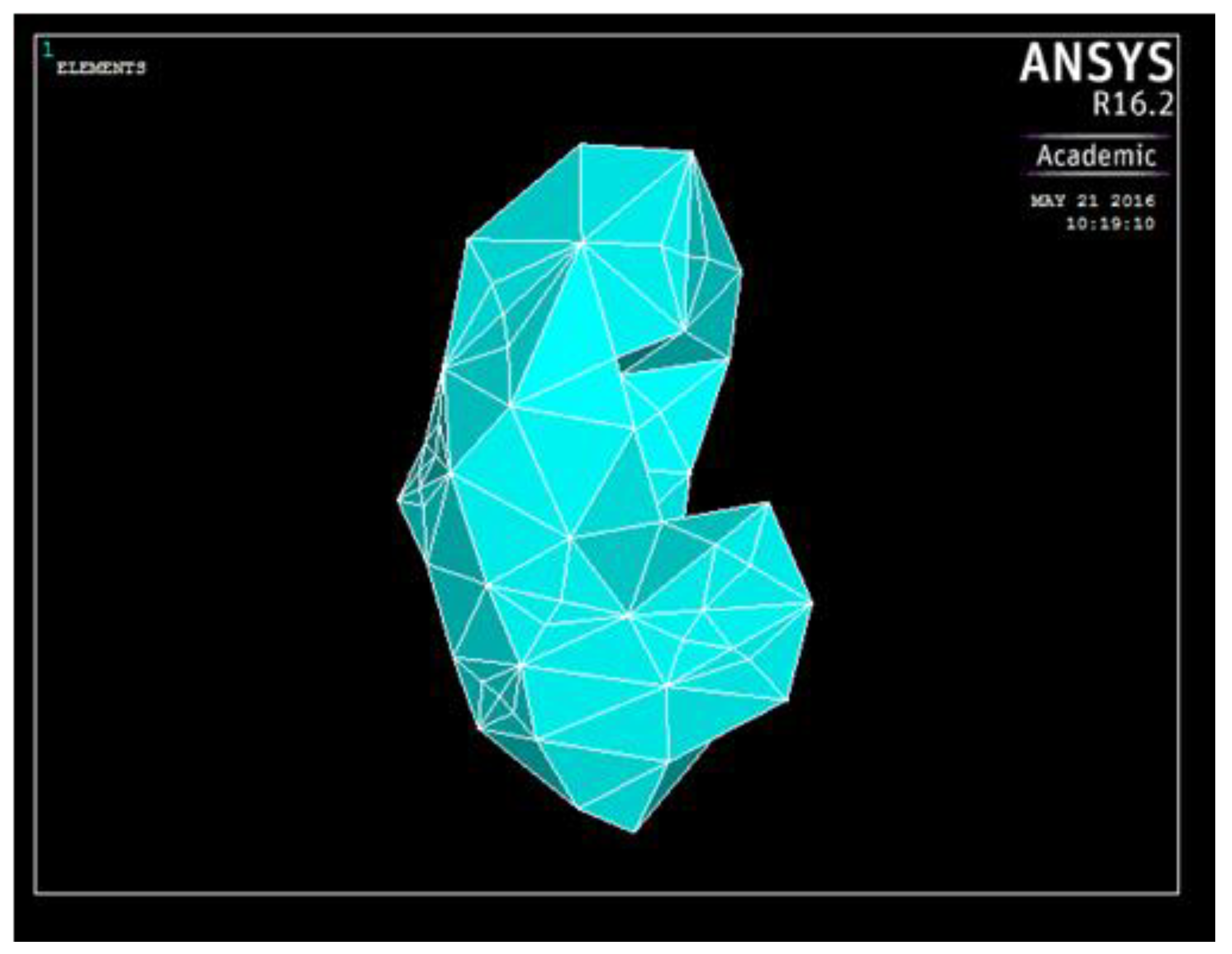
The discretized geometry (undeformed geometry), as displayed in ANSYS, is shown in Figure 2. To get an idea of the size of the geometry and the extent of deformations, one may note that the largest dimension of a typical human kidney is of the order of 100 mm.
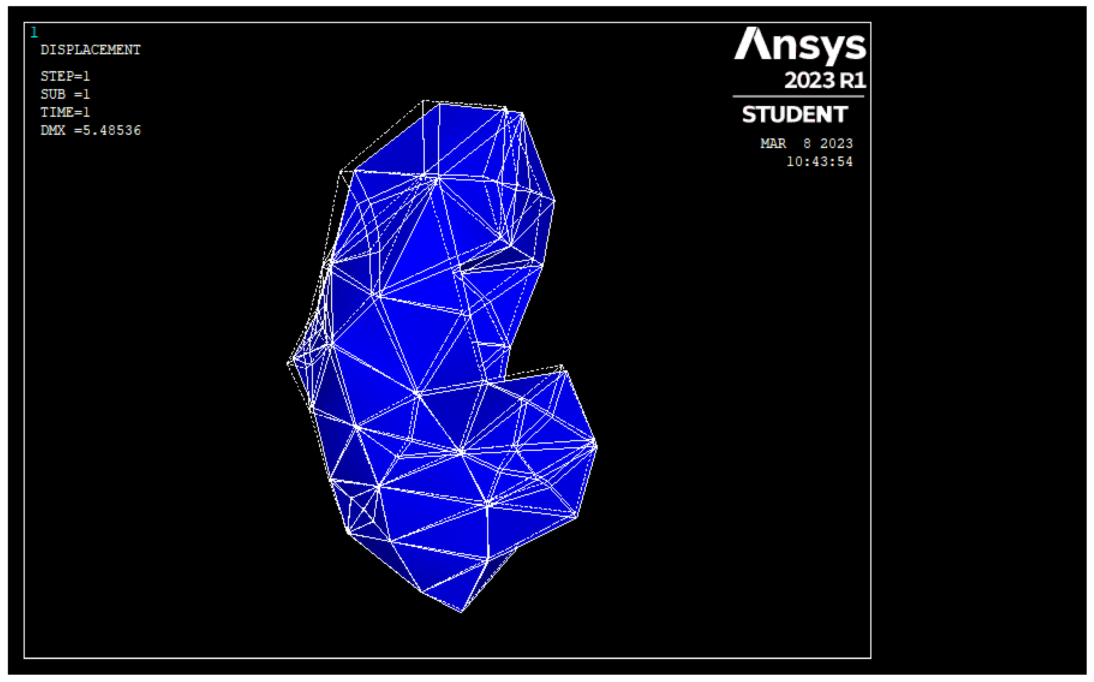
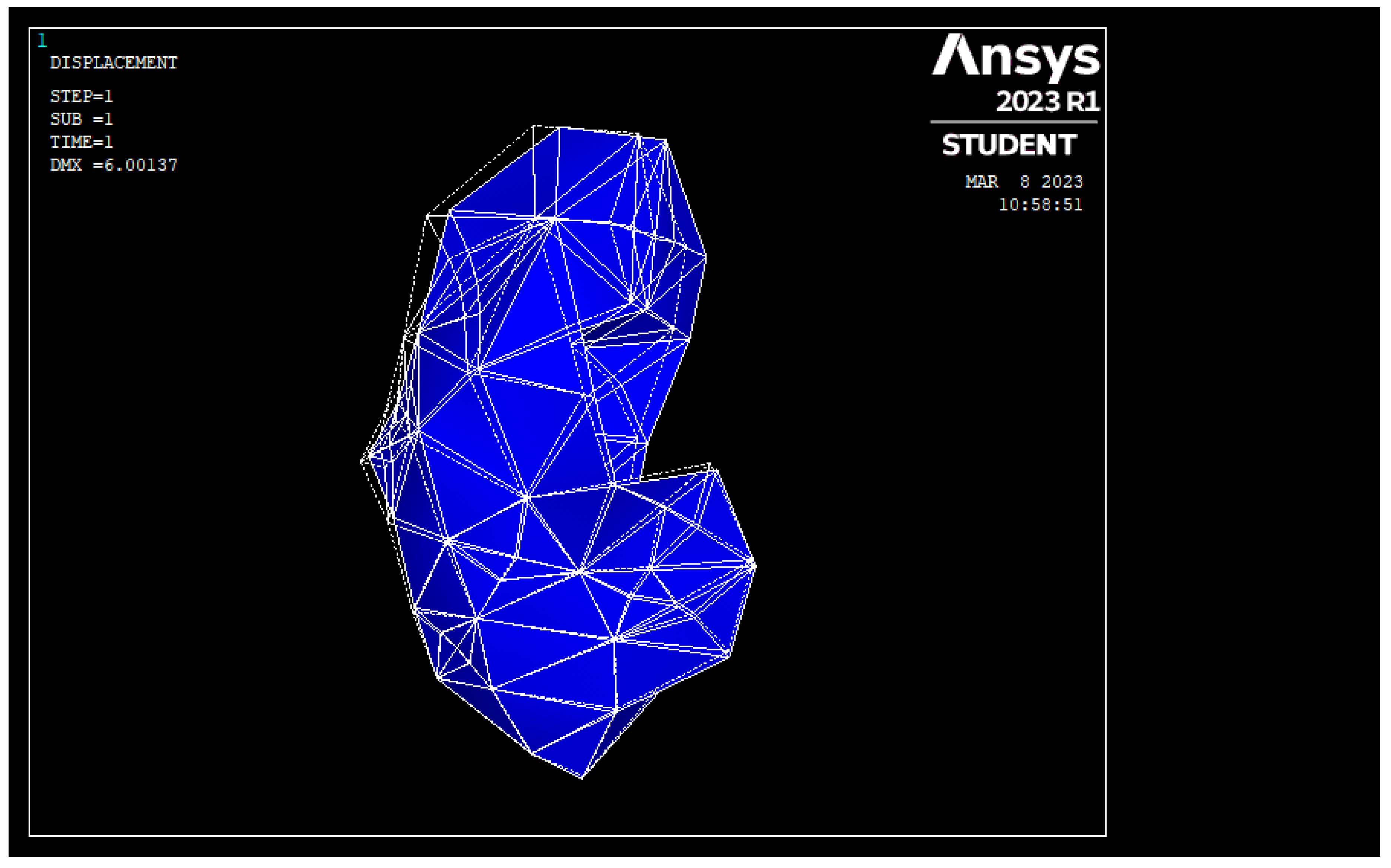
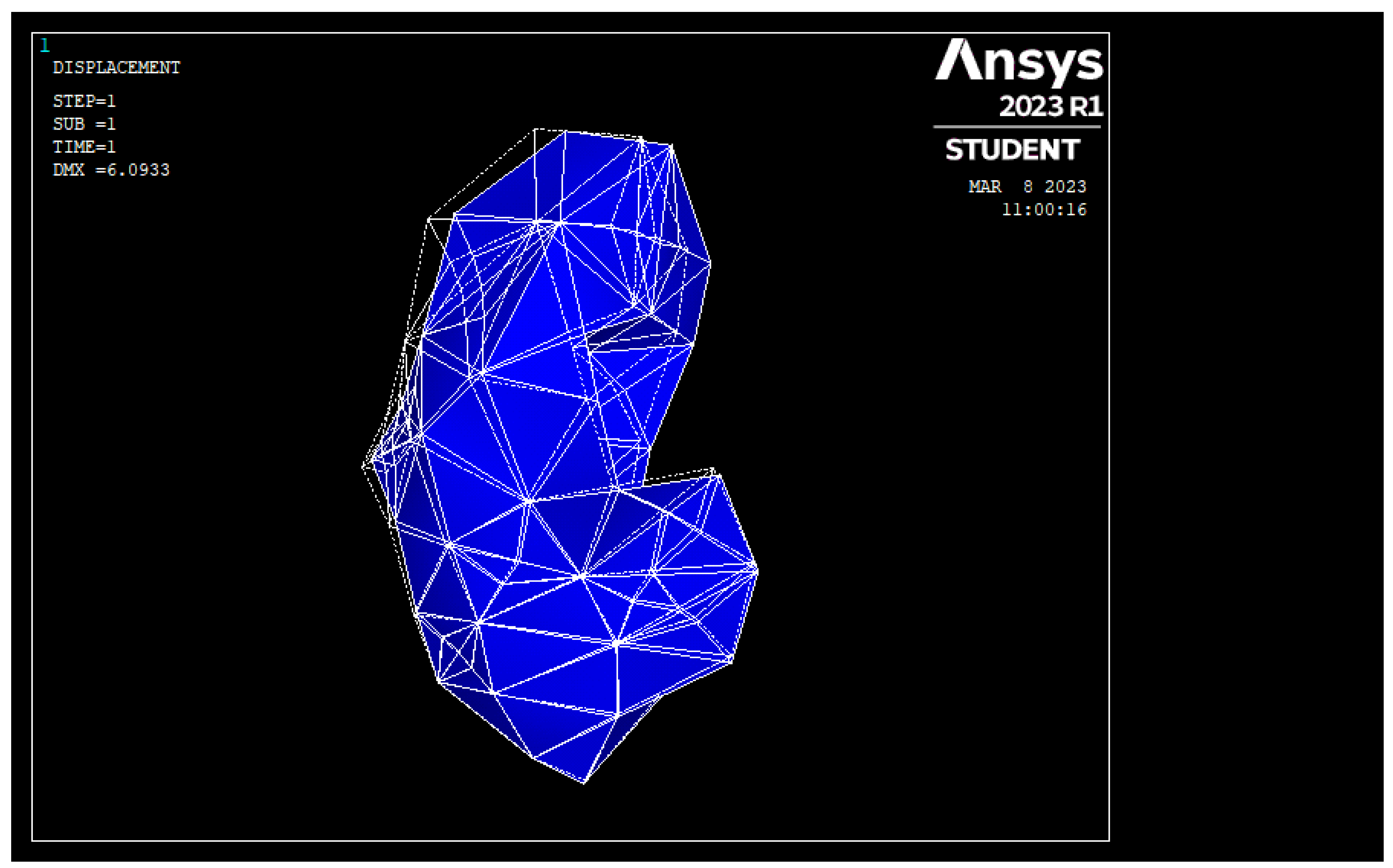
Figure 3 shows the undeformed and deformed geometry, displayed over the same frame, for Problem 1 and for the linear analysis (the rendered mesh refers to the undeformed geometry, whereas the wireframe mesh refers to the deformed geometry). Similarly, Figure 4 shows the undeformed and deformed geometries, displayed over the same frame, for Problem 1 and for the nonlinear analysis (the rendered mesh refers to the undeformed geometry, whereas the wireframe mesh refers to the deformed geometry).
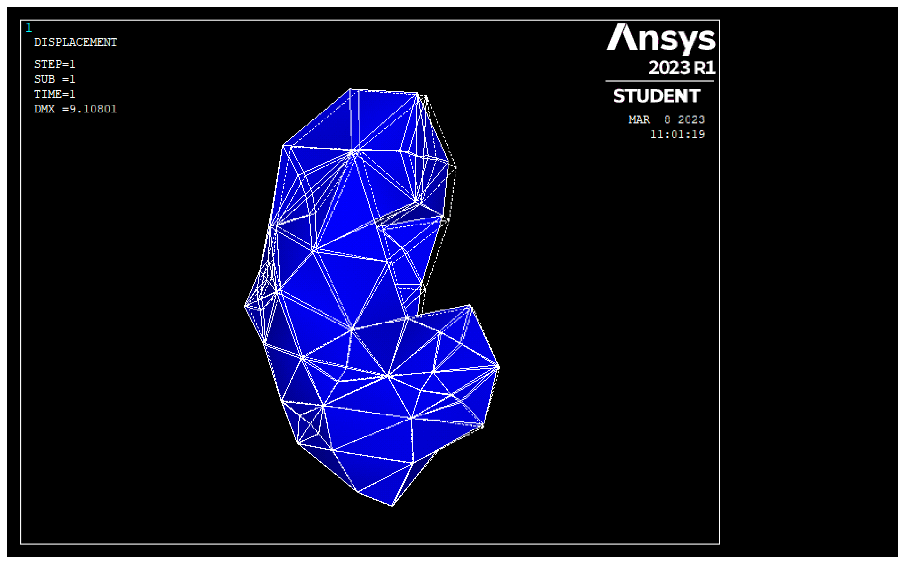
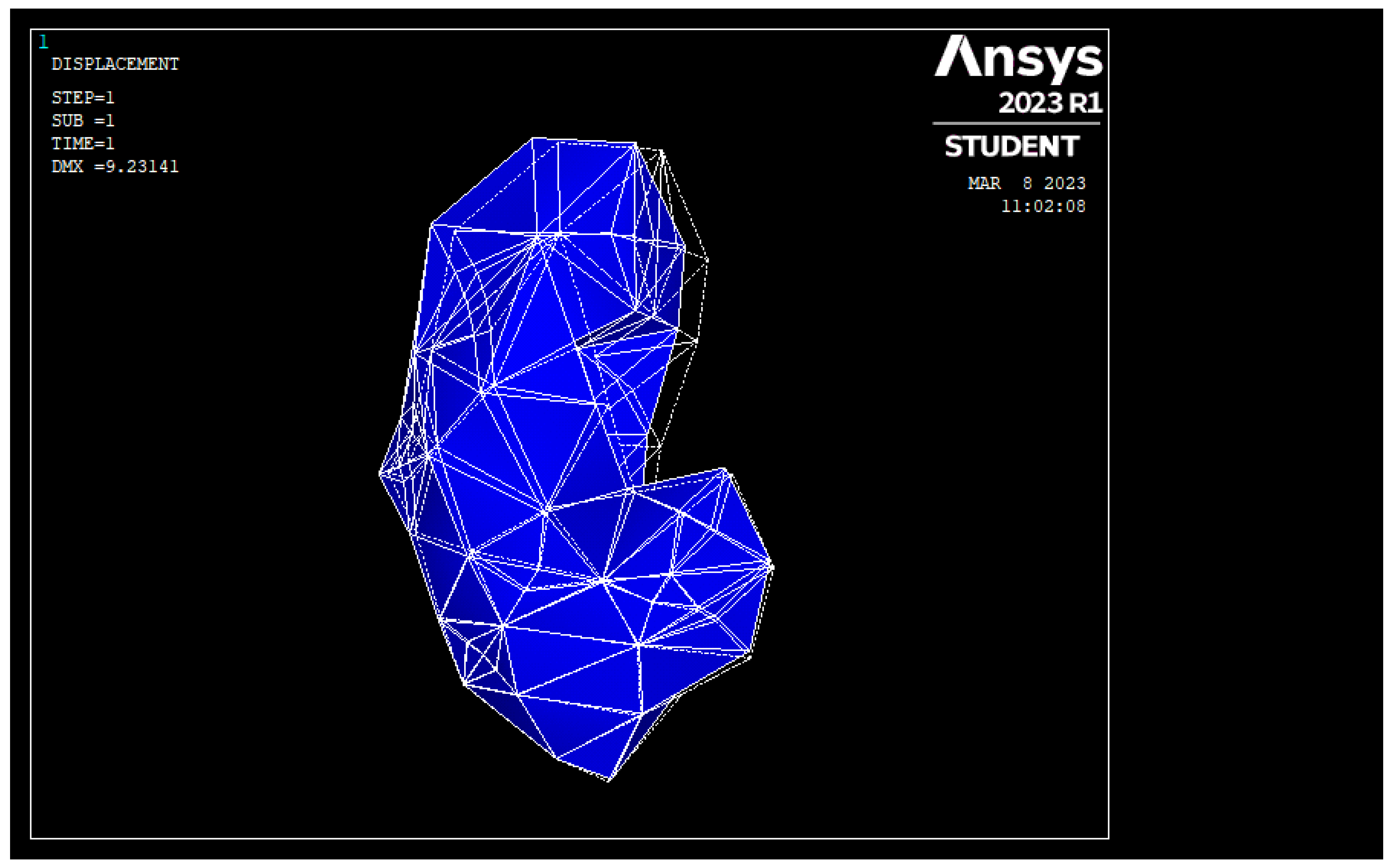
Similarly, Figure 5 shows the undeformed and deformed geometry, for Problem 2 and for the linear analysis (For Figure 5, Figure 6, Figure 7 and Figure 8, the rendered mesh refers to the undeformed geometry whereas the wireframe mesh refers to the deformed geometry). Figure 6 shows the undeformed and deformed geometry for Problem 2 and for the nonlinear analysis. Figure 7 shows the undeformed and deformed geometry for Problem 3 and for the linear analysis. Figure 8 shows the undeformed and deformed geometry for Problem 3 and for the nonlinear analysis.
It is easier to compare the differences between the results from linear and nonlinear analyses if the actual values of the displacements are tabulated. Hence, for each of the analyses above, the values of the displacement vector sum at eleven distinct nodes were noted. These values are tabulated in Table 1, Table 2 and Table 3. The eleven nodes were selected such that they were not from a certain part of the geometry only (i.e., nodes were scattered throughout the geometry). The node numbers of the chosen nodes were 41, 43, 50, 49, 34, 15, 11, 4, 18, 246, 20. The node numbers mentioned here were just the node numbers as named by ANSYS. These nodes were randomly scattered over the entire surface of the kidney. The idea was to try to quantify the deformation of the entire surface of the kidney by noting down the deformation of a few nodes located on the surface of the kidney.
One may note that Figure 3, Figure 4, Figure 5, Figure 6, Figure 7 and Figure 8 plot the deformations considering all the nodes present in the discretized model, but the tables below list the results only for a small representative subset of the total nodes present on the surface of the kidney. Hence, ordering of rows did not matter for the tables, and the node numbers were just the names assigned by ANSYS to a few nodes on the surface of the kidney.
Percentage error in Table 1, Table 2 and Table 3 is relative error, determined with reference to results from a large deformation analysis (i.e., nonlinear analysis). This meant that the error quantified the deviation of results of linear analysis by considering the results from nonlinear analysis as the reference values.
4. Conclusions
From the figures in the last section, deformed geometry obtained by linear analysis appeared to be almost same as the deformed geometry obtained by nonlinear analysis, for all the problems considered. From the tables in the last section, percentage errors were small for most of the nodes considered. However, it was difficult to definitively say how much error was allowed. Only surgeons can say whether a simulation is useful or not. In fact, validating a numerical model by taking feedback from many surgeons, many surgical procedures, and many trials could itself be a research topic. As of present, there is no clarity on what the allowable error in a simulation is, and the subject is a research topic which has not been well explored. However, since linear analysis takes much less time when compared to nonlinear analysis, the results presented in this paper reinforce the idea that just using the linear elastostatic analysis for simulating biological materials could provide usable results quickly and easily. Although preliminary assessments related to the usefulness of the results presented in this paper while building a surgical simulator could have enhanced the utility value of the present study, this author intends to carry out this task in the future (future work).
The results presented in this work could be of use while building simulators that can simulate palpation of liver. As to the limitations of this work, only limited numbers/types of boundary conditions, and only one material model, were considered. Future work could involve considering more boundary conditions and including more material models.
Surgical Simulation is an emerging area that requires fast and accurate simulation of biological materials, and this paper is a small step towards achieving fast and reasonably accurate simulation of biological materials. Although the whole idea of using the finite element method for simulating biological materials is not new, a systematic comparison of the results obtained by using the linear analysis versus the results obtained by using the nonlinear analysis, together with the quantification of errors, is not readily available in the literature and this work assumes significance from that perspective.
Funding
This research received no external funding.
Conflicts of Interest
The authors declare no conflict of interest.
References
- Topalli, D.; Cagiltay, N.E. Eye-hand coordination patterns of intermediate and novice surgeons in a simulation-based endoscopic surgery training environment. J. Eye Mov. Res. 2018, 11, 1. [Google Scholar] [CrossRef] [PubMed]
- Wilson, M.; Coleman, M.; McGrath, J. Developing basic hand-eye coordination skills for laparoscopic surgery using gaze training. BJU Int. 2010, 105, 1356–1358. [Google Scholar] [CrossRef] [PubMed]
- Badash, I.; Burtt, K.; Solorzano, C.A.; Carey, J.N. Innovations in surgery simulation: a review of past, current and future techniques. Ann. Transl. Med. 2016, 4, 453. [Google Scholar] [CrossRef] [PubMed] [Green Version]
- Simbionix Simulators. Available online: https://simbionix.com/simulators/ (accessed on 2 January 2023).
- Surgical Simulation. Available online: https://www.healthysimulation.com/surgical-simulation/ (accessed on 2 January 2023).
- Surgery Simulators. Available online: https://www.medicalexpo.com/medical-manufacturer/surgery-simulator-44251.html (accessed on 2 January 2023).
- Simulation Software for Surgical Training and Education. Available online: https://www.insimo.com/ (accessed on 2 January 2023).
- Surgical Simulation. Available online: https://www.caehealthcare.com/surgical-simulation/ (accessed on 2 January 2023).
- TraumaMan Surgical Simulator. Available online: https://simulab.com/products/traumaman-surgical-simulator (accessed on 2 January 2023).
- Liu, S.; Zhang, Y.; Zheng, W.; Yang, B. Real-time Simulation of Virtual Palpation System. IOP Conf. Series: Earth Environ. Sci. 2019, 234, 12070. [Google Scholar] [CrossRef]
- Moreno-Guerra, M.R.; Martínez-Romero, O.; Palacios-Pineda, L.M.; Olvera-Trejo, D.; Diaz-Elizondo, J.A.; Flores-Villalba, E.; da Silva, J.V.L.; Elías-Zúñiga, A.; Rodriguez, C.A. Soft Tissue Hybrid Model for Real-Time Simulations. Polymers 2022, 14, 1407. [Google Scholar] [CrossRef] [PubMed]
- Mendizabal, A.; Tagliabue, E.; Hoellinger, T.; Brunet, J.-N.; Nikolaev, S.; Cotin, S. Data-driven simulation for augmented surgery. Dev. Nov. Approaches Biomech. Metamaterials 2020, 132, 71–96. [Google Scholar]
- Sacks, M.S.; Motiwale, S.; Goodbrake, C.; Zhang, W. Neural Network Approaches for Soft Biological Tissue and Organ Simulations. J. Biomech. Eng. 2022, 144, 121010. [Google Scholar] [CrossRef] [PubMed]
- Coveney, P.V.; Hoekstra, A.; Rodriguez, B.; Viceconti, M. Computational biomedicine. Part II: organs and systems. Interface Focus 2020, 11, 20200082. [Google Scholar] [CrossRef]
- Zhang, J.; Zhong, Y.; Gu, C. Deformable models for surgical simulation: A survey. IEEE Rev. Biomed. Eng. 2018, 11, 143–164. [Google Scholar] [CrossRef] [PubMed] [Green Version]
- Meier, U.; Lopez, O.; Monserrat, C.; Juan, M.C.; Alcaniz, M. Real-time deformable models for surgery simulation: A survey. Comput. Methods Programs Biomed. 2005, 77, 183–197. [Google Scholar] [CrossRef] [PubMed]
- Delingette, H. Toward realistic soft-tissue modeling in medical simulation. Proc. IEEE 1998, 86, 512–523. [Google Scholar] [CrossRef]
- Villard, P.; Koenig, N.; Perrenot, C.; Perez, M.; Boshier, P. Toward a realistic simulation of organ dissection. Stud. Health Technol. Inf. 2014, 196, 452–456. [Google Scholar]
- Sui, Y.; Pan, J.J.; Qin, H.; Liu, H.; Lu, Y. Real-time simulation of soft tissue deformation and electrocautery procedures in laparoscopic rectal cancer radical surgery. Int. J. Med. Robot. 2017, 13, e1827. [Google Scholar] [CrossRef] [PubMed]
- Chen, X.; Hu, J. A review of haptic simulator for oral and maxillofacial surgery based on virtual reality. Expert Rev. Med. Devices 2018, 15, 435–444. [Google Scholar] [CrossRef] [PubMed]
- Kirana Kumara, P. Studies on the Viability of the Boundary Element Method for the Real-Time Simulation of Biological Organs. Ph.D. Thesis, Centre for Product Design & Manufacturing, Indian Institute of Science, Bangalore, India, 2016. [Google Scholar]
- VHP, n.d. Visible Human Project. Available online: http://www.nlm.nih.gov/research/visible/visible_human.html (accessed on 19 September 2022).
- Kirana Kumara, P. Extracting Three Dimensional Surface Model of Human Kidney from the Visible Human Data Set using Free Software. Leonardo Electron. J. Pract. Technol. 2012, 11, 115–126. [Google Scholar]
- Rasband, W.S.; ImageJ; U.S. National Institutes of Health, Bethesda, Maryland, USA, 1997–2018. Available online: https://imagej.nih.gov/ij/ (accessed on 2 January 2023).
- Schneider, C.A.; Rasband, W.S.; Eliceiri, K.W. NIH Image to ImageJ: 25 years of image analysis. Nat. Methods. 2012, 9, 671–675. [Google Scholar] [CrossRef] [PubMed]
- Yushkevich, P.A.; Piven, J.; Hazlett, H.C.; Smith, R.G.; Ho, S.; Gee, J.C.; Gerig, G. User-guided 3D active contour segmentation of anatomical structures: Significantly improved efficiency and reliability. Neuroimage 2006, 31, 1116–1128. [Google Scholar] [CrossRef] [PubMed] [Green Version]
- Cignoni, P.; Callieri, M.; Corsini, M.; Dellepiane, M.; Ganovelli, F.; Ranzuglia, G. MeshLab: an Open-Source Mesh Processing Tool. In Proceedings of the Sixth Eurographics Italian Chapter Conference, Salerno, Italy, 2–4 July 2008; pp. 129–136. [Google Scholar]
- Rhinoceros. Available online: https://www.rhino3d.com/ (accessed on 2 January 2023).
- Monserrat, C.; Meier, U.; Alcaniz, M.; Chinesta, F.; Juan, M.C. A new approach for the real-time simulation of tissue deformations in surgery simulation. Comput. Methods Programs Biomed. 2001, 64, 77–85. [Google Scholar] [CrossRef] [PubMed]
- Wittek, A.; Hawkins, T.; Miller, K. On the unimportance of constitutive models in computing brain deformation for image-guided surgery. Biomech. Model Mechanobiol. 2009, 8, 77–84. [Google Scholar] [CrossRef] [PubMed] [Green Version]
Figure 1.
Boundary Conditions for the Kidney.

Figure 2.
Discretized Geometry as Displayed in ANSYS.

Figure 3.
Undeformed and Deformed Geometry for Problem 1 (Linear Analysis).

Figure 4.
Undeformed and Deformed Geometry for Problem 1 (Nonlinear Analysis).

Figure 5.
Undeformed and Deformed Geometry for Problem 2 (Linear Analysis).

Figure 6.
Undeformed and Deformed Geometry for Problem 2 (Nonlinear Analysis).

Figure 7.
Undeformed and Deformed Geometry for Problem 3 (Linear Analysis).

Figure 8.
Undeformed and Deformed Geometry for Problem 3 (Nonlinear Analysis).


Table 1.
Percentage Errors for Problem 1.
| Node Number | Displacement Vector Sum for the Large Deformation Analysis (mm) | Displacement Vector Sum for the Small Deformation Analysis (mm) | Percentage Error |
|---|---|---|---|
| 41 | 4.176 | 5.011 | 19.995 |
| 43 | 5.485 | 5.983 | 9.079 |
| 50 | 5.161 | 5.854 | 13.428 |
| 49 | 5.177 | 5.210 | 0.637 |
| 34 | 2.200 | 2.300 | 4.545 |
| 15 | 0.000 | 0.000 | 0.000 |
| 11 | 0.728 | 0.659 | −9.478 |
| 4 | 0.750 | 0.982 | 30.933 |
| 18 | 1.384 | 1.375 | −0.650 |
| 246 | 1.551 | 1.583 | 2.063 |
| 20 | 1.870 | 1.763 | −5.722 |
Table 2.
Percentage Errors for Problem 2.
| Node Number | Displacement Vector Sum for the Large Deformation Analysis (mm) | Displacement Vector Sum for the Small Deformation Analysis (mm) | Percentage Error |
|---|---|---|---|
| 41 | 5.043 | 5.011 | −0.635 |
| 43 | 6.048 | 5.983 | −1.075 |
| 50 | 5.932 | 5.854 | −1.315 |
| 49 | 5.251 | 5.210 | −0.781 |
| 34 | 2.323 | 2.300 | −0.990 |
| 15 | 0.000 | 0.000 | 0.000 |
| 11 | 0.661 | 0.659 | −0.303 |
| 4 | 0.984 | 0.982 | −0.203 |
| 18 | 1.373 | 1.375 | 0.146 |
| 246 | 1.584 | 1.583 | −0.063 |
| 20 | 1.767 | 1.763 | −0.226 |
Table 3.
Percentage Errors for Problem 3.
| Node Number | Displacement Vector Sum for the Large Deformation Analysis (mm) | Displacement Vector Sum for the Small Deformation Analysis (mm) | Percentage Error |
|---|---|---|---|
| 41 | 7.551 | 7.260 | −3.854 |
| 43 | 8.922 | 8.726 | −2.197 |
| 50 | 9.231 | 9.108 | −1.332 |
| 49 | 8.446 | 8.467 | 0.249 |
| 34 | 3.146 | 3.090 | −1.780 |
| 15 | 0.000 | 0.000 | 0.000 |
| 11 | 0.948 | 0.910 | −4.008 |
| 4 | 1.488 | 1.371 | −7.863 |
| 18 | 1.610 | 1.459 | −9.379 |
| 246 | 1.776 | 1.556 | −12.387 |
| 20 | 2.051 | 1.822 | −11.165 |
Disclaimer/Publisher’s Note: The statements, opinions and data contained in all publications are solely those of the individual author(s) and contributor(s) and not of MDPI and/or the editor(s). MDPI and/or the editor(s) disclaim responsibility for any injury to people or property resulting from any ideas, methods, instructions or products referred to in the content. |
© 2023 by the author. Licensee MDPI, Basel, Switzerland. This article is an open access article distributed under the terms and conditions of the Creative Commons Attribution (CC BY) license (https://creativecommons.org/licenses/by/4.0/).
Share and Cite
MDPI and ACS Style
P, K.K. A Comparison between the Results from Linear Analysis and Nonlinear Analysis in the Context of Simulation of Biological Materials. J. Compos. Sci. 2023, 7, 109. https://doi.org/10.3390/jcs7030109
AMA Style
P KK. A Comparison between the Results from Linear Analysis and Nonlinear Analysis in the Context of Simulation of Biological Materials. Journal of Composites Science. 2023; 7(3):109. https://doi.org/10.3390/jcs7030109
Chicago/Turabian StyleP, Kirana Kumara. 2023. "A Comparison between the Results from Linear Analysis and Nonlinear Analysis in the Context of Simulation of Biological Materials" Journal of Composites Science 7, no. 3: 109. https://doi.org/10.3390/jcs7030109