
Development of a Computationally Efficient Model of the Heating Phase in Thermoforming Process Based on the Experimental Radiation Pattern of Heaters

Abstract
:1. Introduction
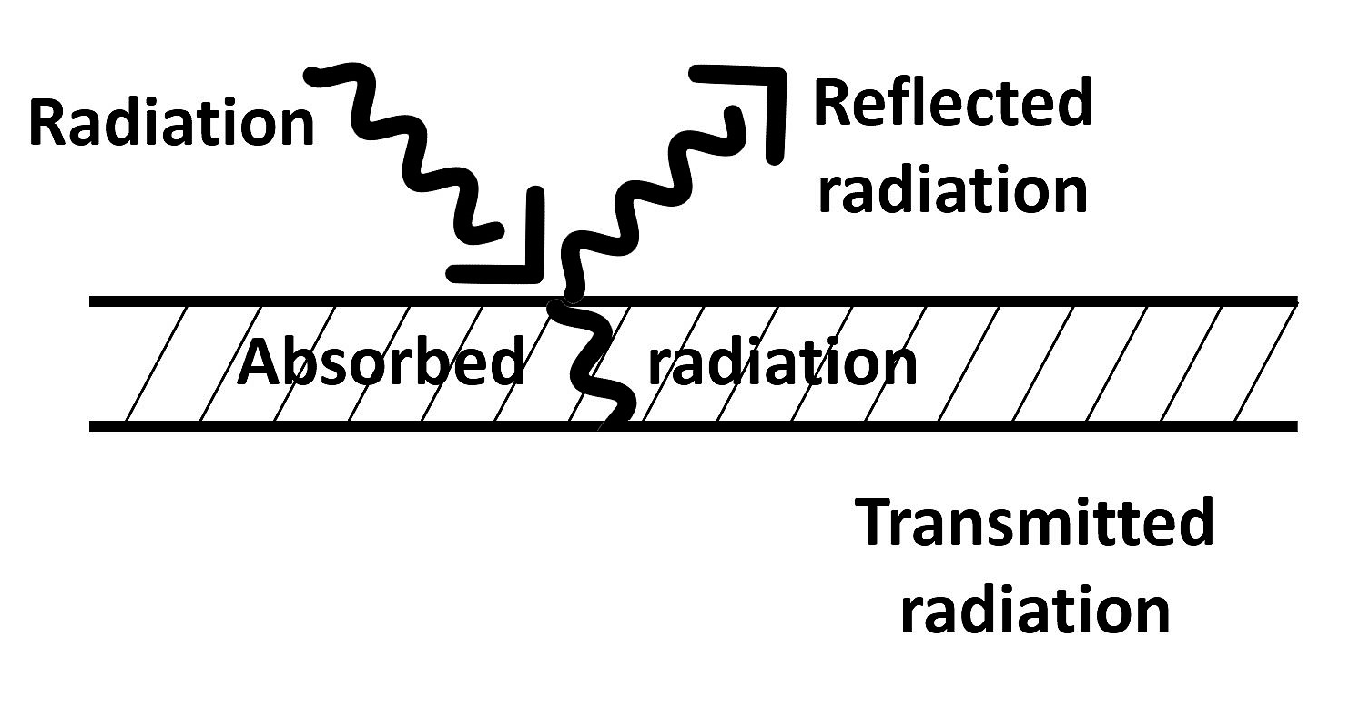
2. Modeling
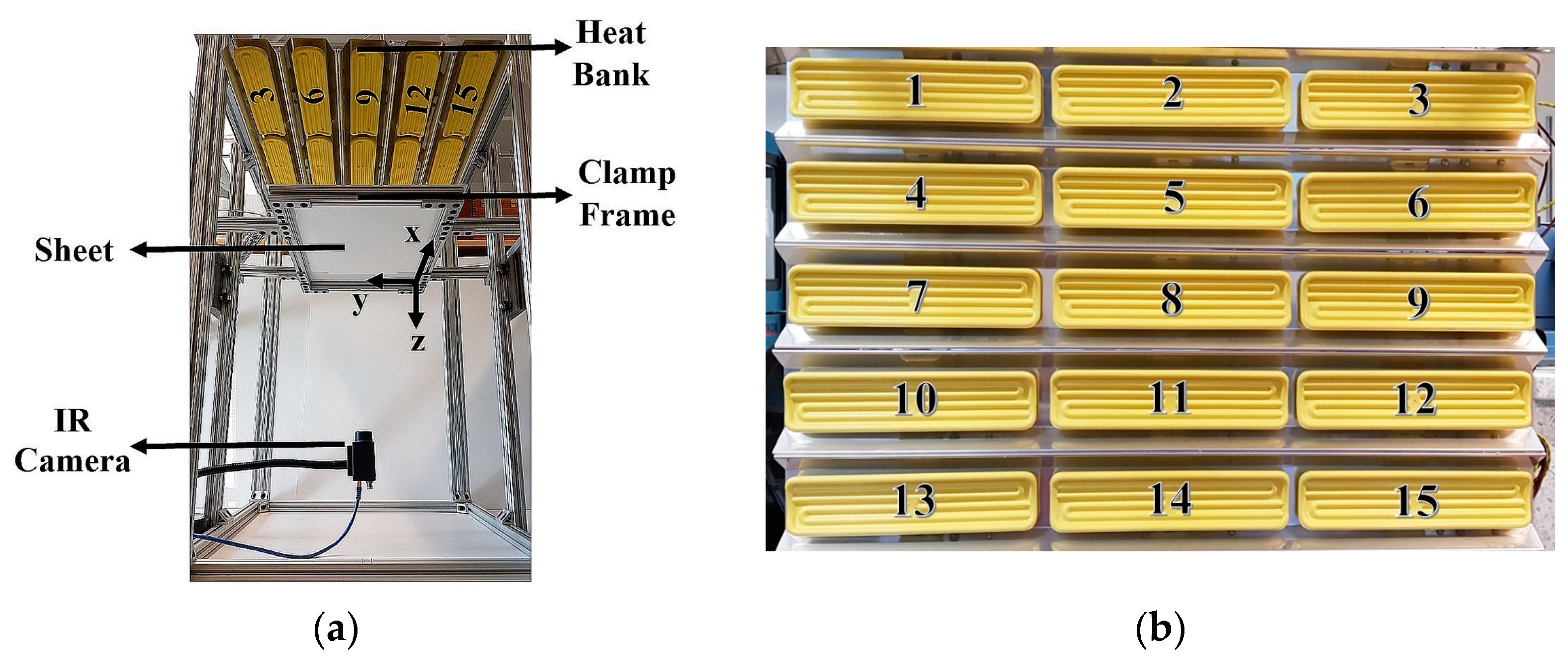
3. Laboratory-Scale Setup
3.1. Heating Element’s Surface Temperature Variation Modelling
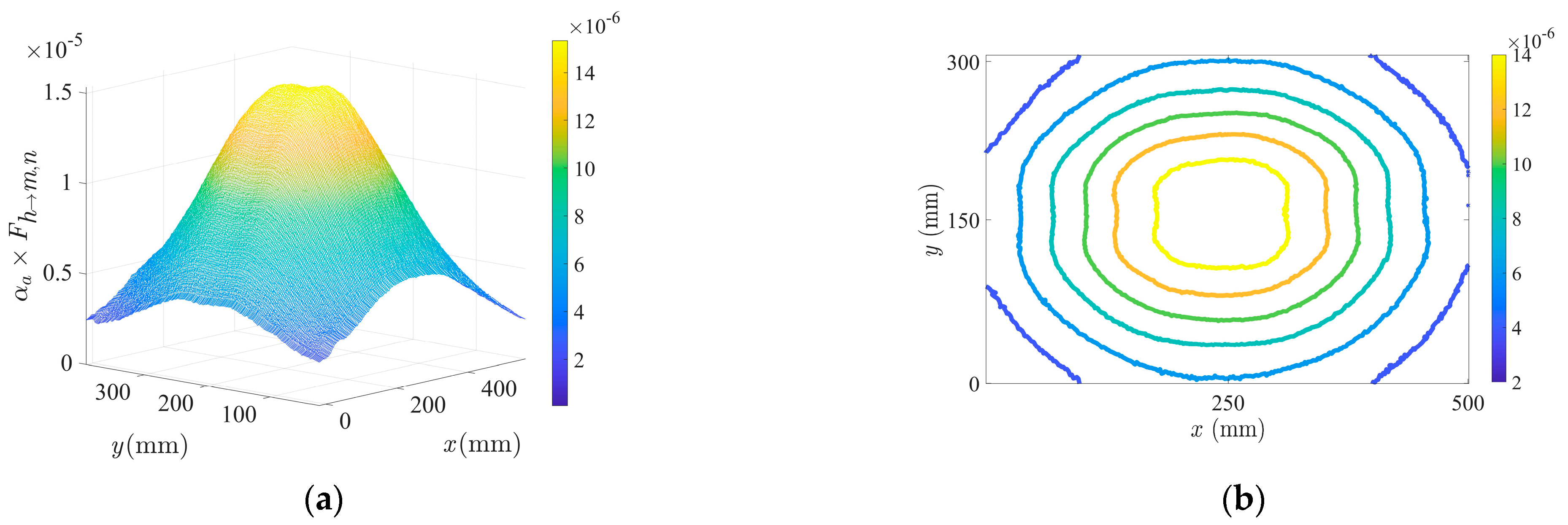
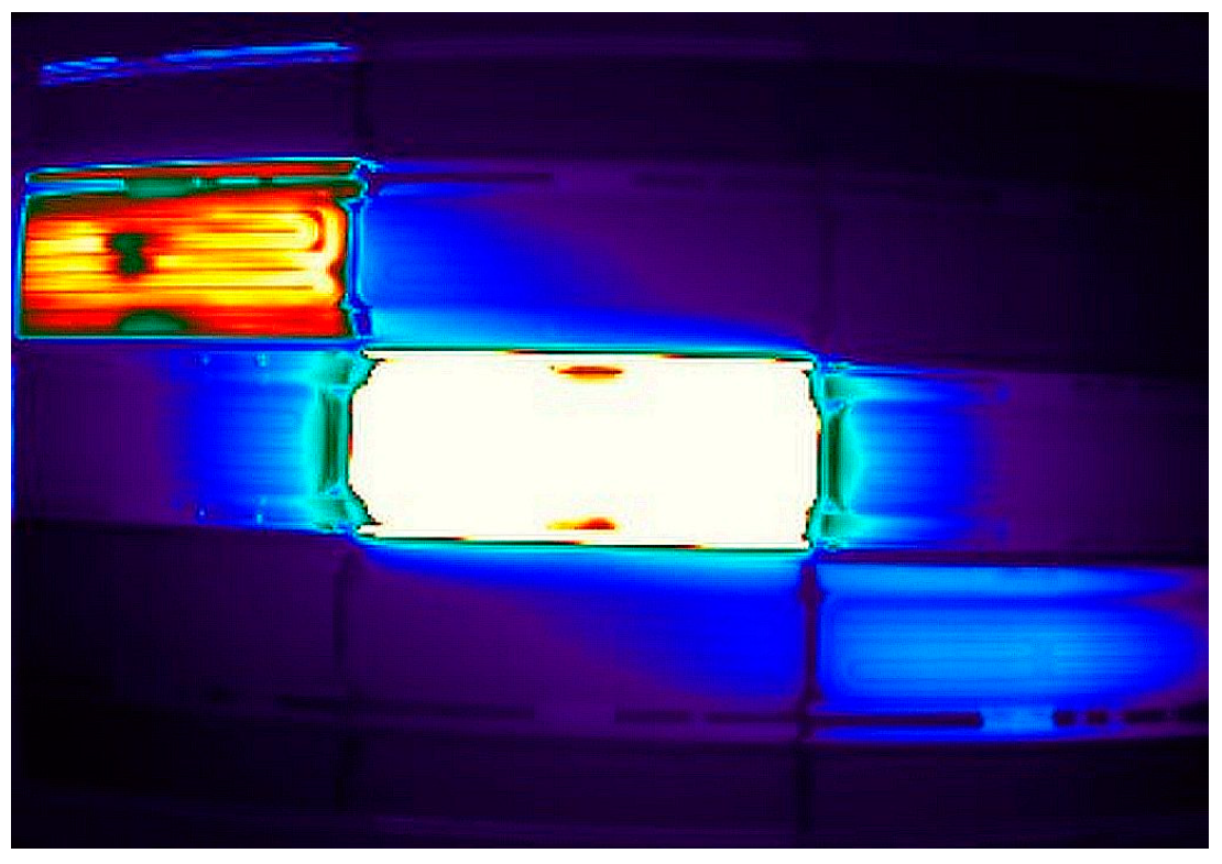
3.2. Experiment to Determine Heating Element’s Radiation Pattern
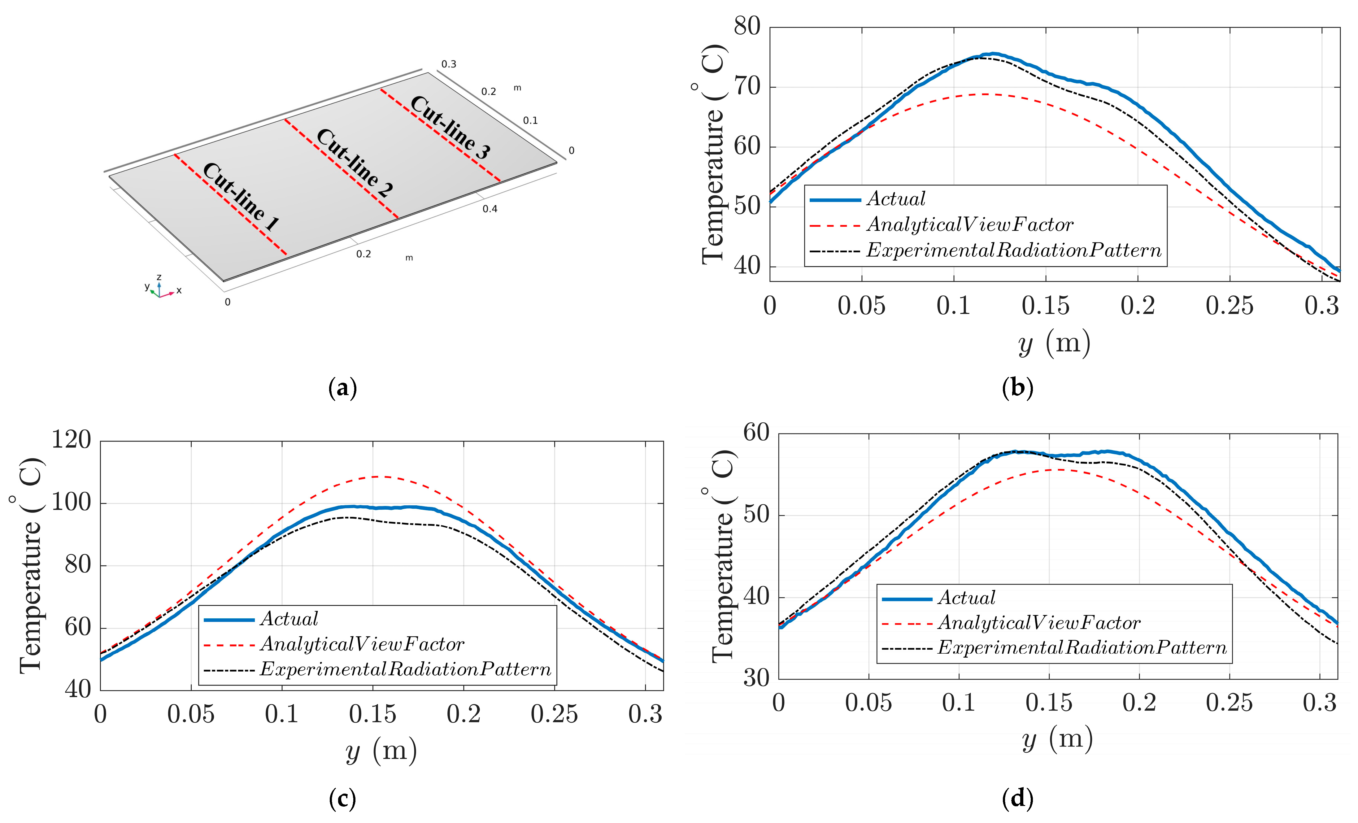
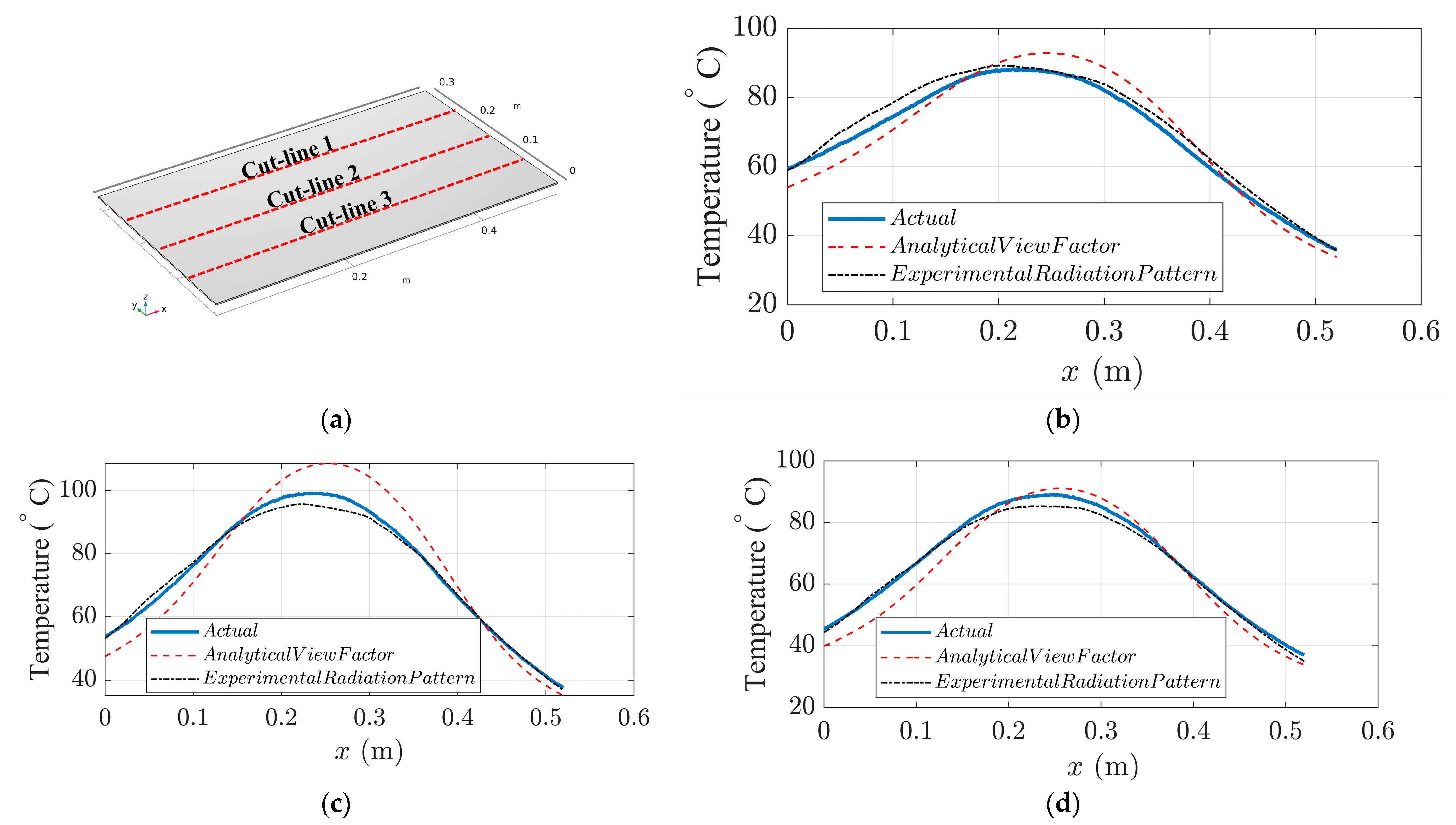
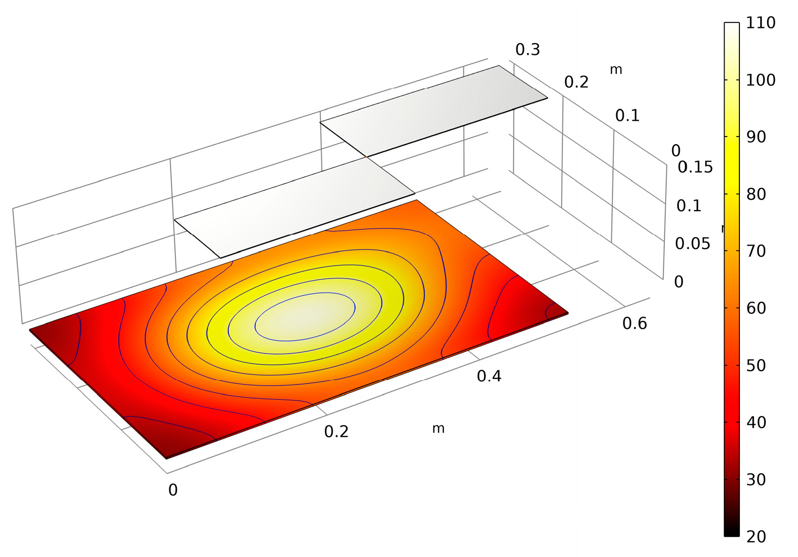
4. Model Verification and Results
5. Discussion and Conclusions
Author Contributions
Funding
Data Availability Statement
Acknowledgments
Conflicts of Interest
References
- Rosin, F.; Forget, P.; Lamouri, S.; Pellerin, R. Enhancing the Decision-Making Process through Industry 4.0 Technologies. Sustainability 2022, 14, 461. [Google Scholar] [CrossRef]
- Forbes, M.G.; Patwardhan, R.S.; Hamadah, H.; Gopaluni, R.B. Model Predictive Control in Industry: Challenges and Opportunities. IFAC-PapersOnLine 2015, 48, 531–538. [Google Scholar] [CrossRef]
- Ramezankhani, M.; Narayan, A.; Seethaler, R.; Milani, A.S. An Active Transfer Learning (ATL) Framework for Smart Manufacturing with Limited Data: Case Study on Material Transfer in Composites Processing. In Proceedings of the 2021 4th IEEE International Conference on Industrial Cyber-Physical Systems (ICPS), Victoria, BC, Canada, 10–12 May 2021; pp. 277–282. [Google Scholar] [CrossRef]
- Ramezankhani, M.; Crawford, B.; Narayan, A.; Voggenreiter, H.; Seethaler, R.; Milani, A.S. Making costly manufacturing smart with transfer learning under limited data: A case study on composites autoclave processing. J. Manuf. Syst. 2021, 59, 345–354. [Google Scholar] [CrossRef]
- Nian, R.; Liu, J.; Huang, B. A review On reinforcement learning: Introduction and applications in industrial process control. Comput. Chem. Eng. 2020, 139, 106886. [Google Scholar] [CrossRef]
- McClement, D.G.; Lawrence, N.P.; Loewen, P.D.; Forbes, M.G.; Backström, J.U.; Gopaluni, R.B. A Meta-Reinforcement Learning Approach to Process Control. IFAC-PapersOnLine 2021, 54, 685–692. [Google Scholar] [CrossRef]
- McClement, D.G.; Lawrence, N.P.; Backström, J.U.; Loewen, P.D.; Forbes, M.G.; Gopaluni, R.B. Meta reinforcement learning for adaptive control: An offline approach. Submitt. J. Process Control. 2022. [Google Scholar] [CrossRef]
- Throne, J.L. (Ed.) Understanding Thermoforming. In Understanding Thermoforming, 2nd ed.; Hanser: München, Wien, 2008; pp. I–XIII. [Google Scholar]
- Throne, J.L. Technology of Thermoforming; Hanser Gardner Publications: Munich, Germany, 1996. [Google Scholar]
- Leite, W.D.O.; Campos Rubio, J.C.; Mata Cabrera, F.; Carrasco, A.; Hanafi, I. Vacuum Thermoforming Process: An Approach to Modeling and Optimization Using Artificial Neural Networks. Polymer 2018, 10, 143. [Google Scholar] [CrossRef]
- Hosseini, H.; Berdyshev, B.V.; Mehrabani-Zeinabad, A. Modeling of Deformation Processes in Vacuum Thermoforming of a Pre-stretched Sheet. Polym. Technol. Eng. 2006, 45, 1357–1362. [Google Scholar] [CrossRef]
- Wang, P.; Hamila, N.; Boisse, P. Thermoforming simulation of multilayer composites with continuous fibres and thermoplastic matrix. Compos. Part B Eng. 2013, 52, 127–136. [Google Scholar] [CrossRef]
- Xiong, H.; Hamila, N.; Boisse, P. Consolidation Modeling during Thermoforming of Thermoplastic Composite Prepregs. Materials 2019, 12, 2853. [Google Scholar] [CrossRef] [PubMed]
- Wang, H.; Li, X.; Phipps, M.; Li, B. Numerical and experimental study of hot pressing technique for resin-based friction composites. Compos. Part A Appl. Sci. Manuf. 2022, 153, 106737. [Google Scholar] [CrossRef]
- Wagner, S.; Kayatz, F.; Münsch, M.; Sanjon, C.W.; Hauptmann, M.; Delgado, A. Numerical modeling of forming air impact thermoforming. Int. J. Adv. Manuf. Technol. 2022, 120, 4917–4933. [Google Scholar] [CrossRef]
- Bean, P.; Lopez-Anido, R.A.; Vel, S. Integration of Material Characterization, Thermoforming Simulation, and As-Formed Structural Analysis for Thermoplastic Composites. Polymers 2022, 14, 1877. [Google Scholar] [CrossRef] [PubMed]
- Buffel, B.; van Mieghem, B.; van Bael, A.; Desplentere, F. A Combined Experimental and Modelling Approach towards an Optimized Heating Strategy in Thermoforming of Thermoplastics Sheets. Int. Polym. Process. 2017, 32, 378–386. [Google Scholar] [CrossRef]
- Wilson, J.; Everett, S.; Dubay, R.; Parsa, S.S.; Tyler, M. Spatial predictive control using a thermal camera as feedback. Measurement 2017, 109, 384–393. [Google Scholar] [CrossRef]
- Shen, Y.-D.; Li, Z.-Z.; Xuan, D.-J.; Heo, K.-S.; Seol, S.-Y. Time-dependent optimal heater control using analytic and numerical methods. Int. J. Precis. Eng. Manuf. 2010, 11, 77–81. [Google Scholar] [CrossRef]
- Li, Z.-Z.; Ma, G.; Xuan, D.-J.; Seol, S.-Y.; Shen, Y.-D. A study on control of heater power and heating time for thermoforming. Int. J. Precis. Eng. Manuf. 2010, 11, 873–878. [Google Scholar] [CrossRef]
- Erchiqui, F.; Hamani, I.; Charette, A. Modélisation par éléments finis du chauffage infrarouge des membranes thermoplastiques semi-transparentes. Int. J. Therm. Sci. 2009, 48, 73–84. [Google Scholar] [CrossRef]
- Venkateswaran, G.; Cameron, M.R.; Jabarin, S.A. Effects of temperature profiles through preform thickness on the proper-ties of reheat-blown PET containers. Adv. Polym. Technol. 1998, 17, 237–249. [Google Scholar] [CrossRef]
- Schmidt, F.; Le Maoult, Y.; Monteix, S. Modelling of infrared heating of thermoplastic sheet used in thermoforming process. J. Mater. Process. Technol. 2003, 143-144, 225–231. [Google Scholar] [CrossRef]
- Duarte, F.; Covas, J.A. IR sheet heating in roll fed thermoforming: Part 1—Solving direct and inverse heating problems. Plast. Rubber Compos. 2002, 31, 307–317. [Google Scholar] [CrossRef]
- Duarte, F.; Covas, J.A. Infrared sheet heating in roll fed thermoforming: Part 2—Factors influencing inverse heating solution. Plast. Rubber Compos. 2003, 32, 32–39. [Google Scholar] [CrossRef]
- Monteix, S.; Schmidt, F.; Le Maoult, Y.; Ben Yedder, R.; Diraddo, R.; Laroche, D. Experimental study and numerical simulation of preform or sheet exposed to infrared radiative heating. J. Mater. Process. Technol. 2001, 119, 90–97. [Google Scholar] [CrossRef]
- Yousefi, A.; Bendada, A.; Diraddo, R. Improved modeling for the reheat phase in thermoforming through an uncertainty treatment of the key parameters. Polym. Eng. Sci. 2002, 42, 1115–1129. [Google Scholar] [CrossRef]
- Gauthier, G.; Ajersch, M.; Boulet, B.; Haurani, A.; Girard, P.; Diraddo, R. A new absorption based model for sheet reheat in thermoforming. In Annual Technical Conference; ANTEC: Boston, MA, USA, 2005. [Google Scholar]
- Chy, M.I.; Boulet, B. Development of an improved mathematical model of the heating phase of thermoforming process. In Proceedings of the 2011 IEEE Industry Applications Society Annual Meeting, Orlando, FL, USA, 9–13 October 2011; pp. 1–8. [Google Scholar] [CrossRef]
- Erchiqui, F. Application of genetic and simulated annealing algorithms for optimization of infrared heating stage in thermoforming process. Appl. Therm. Eng. 2018, 128, 1263–1272. [Google Scholar] [CrossRef]
- Erchiqui, F.; Ngoma, G.D. Analyse comparative des méthodes de calcul des facteurs de formes pour des surfaces à contours rectilignes. Int. J. Therm. Sci. 2007, 46, 284–293. [Google Scholar] [CrossRef]
- Ehlert, J.R.; Smith, T.F. View factors for perpendicular and parallel rectangular plates. J. Thermophys. Heat Transf. 1993, 7, 173–175. [Google Scholar] [CrossRef]
- Rodrigues, J.D.S.; Gonçalves, P.T.; Pina, L.; de Almeida, F.G. Modelling the Heating Process in the Transient and Steady State of an In Situ Tape-Laying Machine Head. J. Manuf. Mater. Process. 2022, 6, 8. [Google Scholar] [CrossRef]
- Holman, J.P. Heat Transfer; McGraw-Hill: New York, NY, USA, 2009. [Google Scholar]
- Poelma, R.H.; Tarashioon, S.; Van Zeijl, H.W.; Goldbach, S.; Zijl, J.L.J.; Zhang, G.Q. Multi-LED package design, fabrication and thermal analysis. J. Semicond. 2013, 34, 54002. [Google Scholar] [CrossRef]
- Michael, F. Modest: Radiative Heat Transfer; Elsevier: Amsterdam, The Netherlands, 2003. [Google Scholar]
- Howell, J.R.; Mengüç, M.P.; Daun, K.; Siegel, R. Thermal Radiation Heat Transfer, 7th ed.; CRC Press: Boca Raton, FL, USA, 2021; Revised edition of: Thermal radiation heat transfer/John R. Howell, M. Pinar Mengüç, Robert Siegel; Sixth edition. 2015. (2020). [Google Scholar]
- Ivanova, S.M.; Muneer, T. Finite-element heat-transfer computations for parallel surfaces with uniform or non-uniform emitting. J. Renew. Sustain. Energy 2016, 8, 015102. [Google Scholar] [CrossRef]
- Ceramicx Company. Available online: https://www.ceramicx.com/ (accessed on 1 September 2022).
- COMSOL. Multiphysics® v. 5.6; COMSOL AB: Stockholm, Sweden; Available online: www.comsol.com (accessed on 1 September 2022).
- Rashidi, A.; Milani, A.S. Passive control of wrinkles in woven fabric preforms using a geometrical modification of blank holders. Compos. Part A Appl. 2018, 105, 300–309. [Google Scholar] [CrossRef]
- Daghigh, H.; Daghigh, V.; Milani, A.; Tannant, D.; Lacy, V.C., Jr.; Reddy, N.J. Nonlocal bending and buckling of agglomerated CNT-reinforced composite nanoplates. Compos. B. Eng. 2020, 183, 107716. [Google Scholar] [CrossRef]


| Direction | Symbol | Value | Unit |
|---|---|---|---|
| Thermal Conductivity | 0.18 | ||
| Specific Heat | 1465 | ||
| Density | 1380 | ||
| Emissivity | 0.95 | - |
| #Heater | Power Consumption (W) | Heaters’ Surface Temperature (K) |
|---|---|---|
| 4 | 200 | 603 |
| 8 | 500 | 803 |
| Vertical Cut-Lines | Horizontal Cut-Lines | |||||||
|---|---|---|---|---|---|---|---|---|
| Experimental Radiation Pattern | Analytical View Factors | Experimental Radiation Pattern | Analytical View Factors | |||||
| MSE | RMSE | MSE | RMSE | MSE | RMSE | MSE | RMSE | |
| Cut-line 1 | 4.3 | 2.07 | 22.2 | 4.71 | 5.5 | 2.34 | 16.2 | 4.02 |
| Cut-line 2 | 10.4 | 3.22 | 23.7 | 4.86 | 3.8 | 1.94 | 40.5 | 6.36 |
| Cut-line 3 | 2.4 | 1.54 | 5.7 | 2.38 | 3.4 | 1.84 | 16.8 | 4.09 |
Disclaimer/Publisher’s Note: The statements, opinions and data contained in all publications are solely those of the individual author(s) and contributor(s) and not of MDPI and/or the editor(s). MDPI and/or the editor(s) disclaim responsibility for any injury to people or property resulting from any ideas, methods, instructions or products referred to in the content. |
© 2023 by the authors. Licensee MDPI, Basel, Switzerland. This article is an open access article distributed under the terms and conditions of the Creative Commons Attribution (CC BY) license (https://creativecommons.org/licenses/by/4.0/).
Share and Cite
Hosseinionari, H.; Ramezankhani, M.; Seethaler, R.; Milani, A.S. Development of a Computationally Efficient Model of the Heating Phase in Thermoforming Process Based on the Experimental Radiation Pattern of Heaters. J. Manuf. Mater. Process. 2023, 7, 48. https://doi.org/10.3390/jmmp7010048
Hosseinionari H, Ramezankhani M, Seethaler R, Milani AS. Development of a Computationally Efficient Model of the Heating Phase in Thermoforming Process Based on the Experimental Radiation Pattern of Heaters. Journal of Manufacturing and Materials Processing. 2023; 7(1):48. https://doi.org/10.3390/jmmp7010048
Chicago/Turabian StyleHosseinionari, Hadi, Milad Ramezankhani, Rudolf Seethaler, and Abbas S. Milani. 2023. "Development of a Computationally Efficient Model of the Heating Phase in Thermoforming Process Based on the Experimental Radiation Pattern of Heaters" Journal of Manufacturing and Materials Processing 7, no. 1: 48. https://doi.org/10.3390/jmmp7010048