Article

Using 3D Density-Gradient Vectors in Evolutionary Topology Optimization to Find the Build Direction for Additive Manufacturing

Department of Mechanical and Manufacturing Engineering, Ontario Tech University, Faculty of Engineering and Applied Science, North Campus, Oshawa, ON L1G 0C5, Canada
*
Author to whom correspondence should be addressed.
J. Manuf. Mater. Process. 2023, 7(1), 46; https://doi.org/10.3390/jmmp7010046
Submission received: 25 December 2022 / Revised: 1 February 2023 / Accepted: 2 February 2023 / Published: 9 February 2023

Abstract

:
Given its layer-based nature, additive manufacturing is known as a family of highly capable processes for fabricating complex 3D geometries designed by means of evolutionary topology optimization. However, the required support structures for the overhanging features of these complex geometries can be concerningly wasteful. This article presents an approach for studying the manufacturability of the topology-optimized complex 3D parts required for additive manufacturing and finding the optimum corresponding build direction for the fabrication process. The developed methodology uses the density gradient of the design matrix created during the evolutionary topology optimization of the 3D domains to determine the optimal build orientation for additive manufacturing with the objective of minimizing the need for support structures. Highly satisfactory results are obtained by implementing the developed methodology in analytical and experimental studies, which demonstrate potential additive manufacturing mass savings of 170% of the structure’s weight. The developed methodology can be readily used in a variety of evolutionary topology optimization algorithms to design complex 3D geometries for additive manufacturing technologies with a minimized level of waste due to reducing the need for support structures.

1. Introduction

Topology optimization is a form of design optimization that seeks to achieve the best performance for a structural part or mechanical component by determining the best locations and geometries of cavities within the design domain while satisfying various constraints [1]. Figure 1 demonstrates the process of defining the design problem, discretizing the design domain into finite elements, and then performing topology optimization to achieve an efficient structure. Many methods of topology optimization, including the Homogenization Method, Bi-Directional Evolutionary Structural Optimization Method (BESO), Solid Isotropic Material with Penalization (SIMP), Level Set, and Phase Field, are currently employed in various design problems, and very successful results have been reported [2]. However, regardless of the optimization method, the complex geometries created by topology optimization are mainly very difficult to manufacture. Traditional manufacturing technologies are typically not flexible enough to fabricate the complex topologically optimized parts at an affordable cost. The highly efficient topologies achieved through topology optimization often come with geometric complexities that are difficult or even impossible to manufacture using traditional manufacturing techniques. Among the manufacturing processes, the emerging field of Additive Manufacturing (AM) allows for ease of manufacturing that is mostly independent of the part’s complexity. The flexibility within AM processes is mainly due to their nature of manufacturing by addition.
AM, which is also referred to as 3D printing, is currently a cost-effective way to produce plastic, metal, ceramic, and composite parts of high complexity and small batch size in many novel fields [3,4]. Combined with topology optimization, it has great potential to replace conventional manufacturing and design processes [5]. The AM processes rely on layer-by-layer material deposition or solidification, which provides a designer with many advantages over traditional manufacturing processes, such as part consolidation, weight reduction, functional customization, personalization, and aesthetics [6,7], although it is not without its own limitations, such as the need for support material and poor surface finish quality [8,9,10,11]. Among these issues, the need for supporting structures for fabricated overhanging features is one of the most concerning ones, since these supports are mainly considered a waste in terms of the use of material, processing time, and post-processing required to remove them and finish the affected surfaces on the final product [12,13].
This article presents an approach for studying the manufacturability of the topology-optimized complex 3D parts for AM and demonstrating its applicability by finding the optimum build direction for the fabrication process. The developed methodology analyzes the density field of the design domain generated and used during typical evolutionary topology optimization processes [14,15]. The SIMP method assumes that each element of the discretized design domain contains an isotropic material with a variable density, where the material properties are assumed to be constant within each element and the design variables are the element’s relative densities. The material properties are modelled as the relative material density raised to some power [2].
Although, the recent developments in topology optimization have been very successful in designing complex structures with the highest levels of efficiencies, the resulting designs cannot be always used when there is no feasible or economically viable manufacturing and quality assurance process in place to support developing a final product. In term of manufacturability analyses, the complex topologies typically result in difficult to manufacture features. There have been significant research works to understand the geometric features and characteristics that make the manufacturing unfeasible to expensive, as the manufacturability limitations [16]. As the next step, the manufacturing limitations are typically introduced to in the design process as the design constraints. Considering the requirement for quality assurance, it is highly important to guarantee a way that complex structure resulting by topology optimization can be inspected after or during the manufacturing process. This includes the considerations corresponding the inspections tools and methods, sampling strategy, and the ways to evaluate the inspection data [17,18,19]. Although the focus of this work is on the manufacturability of the complex topologies resulting by topology optimization, the same level of attention is needed to the inspection-ability of these topologies. Analyzing the manufacturability of the complex structures resulting from topology optimization is a crucial task. Additive manufacturing has been known as one of the most reliable technologies for manufacturing topology-optimized 3D structures [5]. However, AM’s limitations and constraints, including the need for structural support during the fabrication process, require more attention from researchers. One of the main topics is the consideration of overhanging surfaces where the effect of the inclined angle of the overhanging surface directly correlates with the need for a supporting structure. This phenomenon was experimentally studied on a direct metal laser sintering machine by Wang et al. [20]. Their research found that overhanging surfaces induce higher residual stresses and warp easier as the inclined angle becomes smaller relative to the build platform. In order to prevent small, inclined build angles from warping, an additional support structure should be included alongside the main part being printed. The support structure is often a scaffolding-like lattice structure erected from the build platform to the overhanging surface, and it is often printed using the base material. This supporting structure adds to the required time to print the material, increases the wasted material, increases the post processing times, and negatively affects the surface finish of the part [21]. For these reasons, as well as the increasing popularity of AM in academia and industry, topology optimization with AM constraints has been extensively researched in recent years [22].
Using the elemental density gradient vectors to analyze the angles of overhanging surfaces has been addressed in some research works on 2D topology optimization. To the best of the authors’ knowledge, the first mention of using this method was made by Leary et al. [23], who used local gradient information to identify the regions of the theoretically optimal topology and modify it as required to ensure manufacturability without requiring additional support material. Driessen [24] and Garaigordobil et al. [25] have used the gradient of the density field to formulate an overhang constraint to produce self-supporting designs, that is, designs which can be 3D printed without any supporting structure. Mass and Amir [26] used similar density gradient approximation techniques in the continuum portion of their two-step process for morphing their structural design toward one that is self-supporting. Qian [27] used the density gradients to check the undercuts and overhangs and then applied Heaviside projection to form a global constraint. Bender and Barari [28] used the density gradient at the perimeter of the final structure to identify the locations and, in turn, the required volume of the supporting structure, which they then used to perform support slimming by means of orientation optimization relative to the print direction. This approach minimizes the required volume of supporting structure.
The methods mentioned above are presented in 2D problems. The likely reason for the lack of 3D implementation has been the need to approximate the density gradient in a 3D space. Image processing techniques have been mainly used to develop the density gradient matrix [29], which is only performed in two dimensions to address the rows and columns of a picture, when a structural analysis should be performed in the three cartesian dimensions.
An extension of the 2D image processing gradient approximation method into 3D applications is herein presented using matrix convolution with kernels. The applicability of the density gradient vectors derived from a uniquely topology-optimized structure is demonstrated for additive manufacturing by setting up a basic support slimming algorithm based on the overhanging angles relative to the build direction. The density gradient vector approximation method is then presented in a filter-based approach such as the ones commonly implemented in common topology optimization algorithms.

2. Theoretical Background

Additive manufacturing is a cost-effective way to produce small batches, with the manufacturing costs being almost completely decoupled from the geometric complexity and assembly status of the products [30,31,32]. Although AM provides many advantages over traditional manufacturing techniques, it is not without its own drawbacks, which are best outlined in the context of topology optimization in [28], as well as deviations from the true geometry from manufacturing artifacts such as the “staircase effect” and others. These properties of AM synergize with structural topology optimization to easily produce normally un-manufacturable or difficult to manufacture parts, sub-assemblies, and assemblies with complex shapes and geometries, which are often resulting features of topology optimization.

2.1. Topology Optimization

A density-based power law approach to topology optimization known as the Simple Isotropic Material with Penalization (SIMP) method was implemented to develop the presented algorithm. An advantage of using the SIMP method is that it allows for the straightforward implementation of additional filters [33,34].
The first step in any structural design process is to define the design problem and its subsequent design domain. Once the structural design problem has been constructed, the design domain is then discretized to perform a finite element analysis of the structure, such as that in Figure 2. The discretized design domain may consist of elements of four or more nodes with any number of elements, but often in research applications, cube elements are implemented with eight nodes and the number of elements is limited by the available computational power. Again, for the sake of simplicity, each node of an element will contain 3 degrees of freedom (translation along the 3 Cartesian axes) where the forces and boundary conditions of the design problem are applied. Finite element methods are then implemented to determine the nodal displacement vector, u , and the elemental stiffness matrices, K e . The topology optimization techniques employed use the results of the finite element analysis to slightly modify the design domain from the current iteration to the next. The stiffness matrix and displacement vector of the new structure are then calculated, and the process of finite element analysis and design modification repeats itself until the convergence criteria have been met.
The SIMP method of topology optimization modifies the relative densities, ρ , of each element of the discretized design domain, where a relative density of zero implies that an element is fully void, a relative density of one represents a fully solid element, and a density between zero and one is an element somewhere between fully void and fully solid. The densities of the elements are used to interpolate the Young’s modulus, E , of an element, which implies that as the density of an element increases, so does its stiffness. These equations for topology optimization can be found in [1]. The relationship between an element’s stiffness and density is given by
E ρ e = E m i n + ρ e p E 0 E m i n  
where E m i n and E 0 are the elastic Young’s modulus of the void and solid material, respectively, and ρ e   is the elemental density. The penalization power, p , is taken to be a real value greater than one, and it is implemented to steer the solution to a nearly solid-void design [35].
The formulation of the topology optimization problem is as follows.
Minimize:
c = f T u  
Subject to:
V * e = 1 N v e ρ e  
0 < ρ m i n   ρ e   1  
where N is the total number of discrete elements and c is the stiffness compliance of the structure (an inverse measure of stiffness) calculated using the transposed nodal force and displacement vectors, f T and u , respectively. V * is the prescribed total structural volume and v e is the volume of an individual element of the discretized design domain.
The sensitivity of the objective function, c , for each element, e , is found to be
c x i = p ρ e p 1 u e T K e 0 u e  
The optimization problem is solved using a heuristic updating scheme known as the optimality criteria. The optimizer redistributes the density in the design domain to give elements with higher sensitivity numbers more density and, conversely, lower the density of elements with low sensitivity values. A more detailed explanation of the optimality criteria and their counterparts can be found in [34].

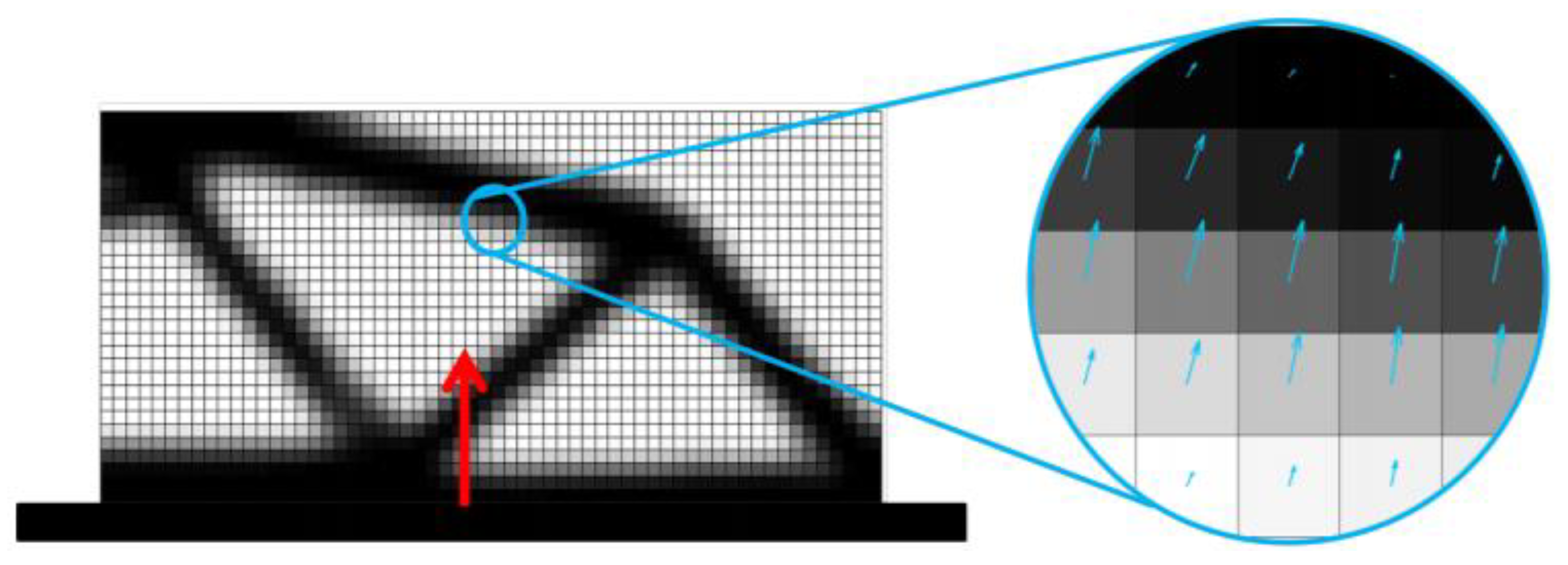
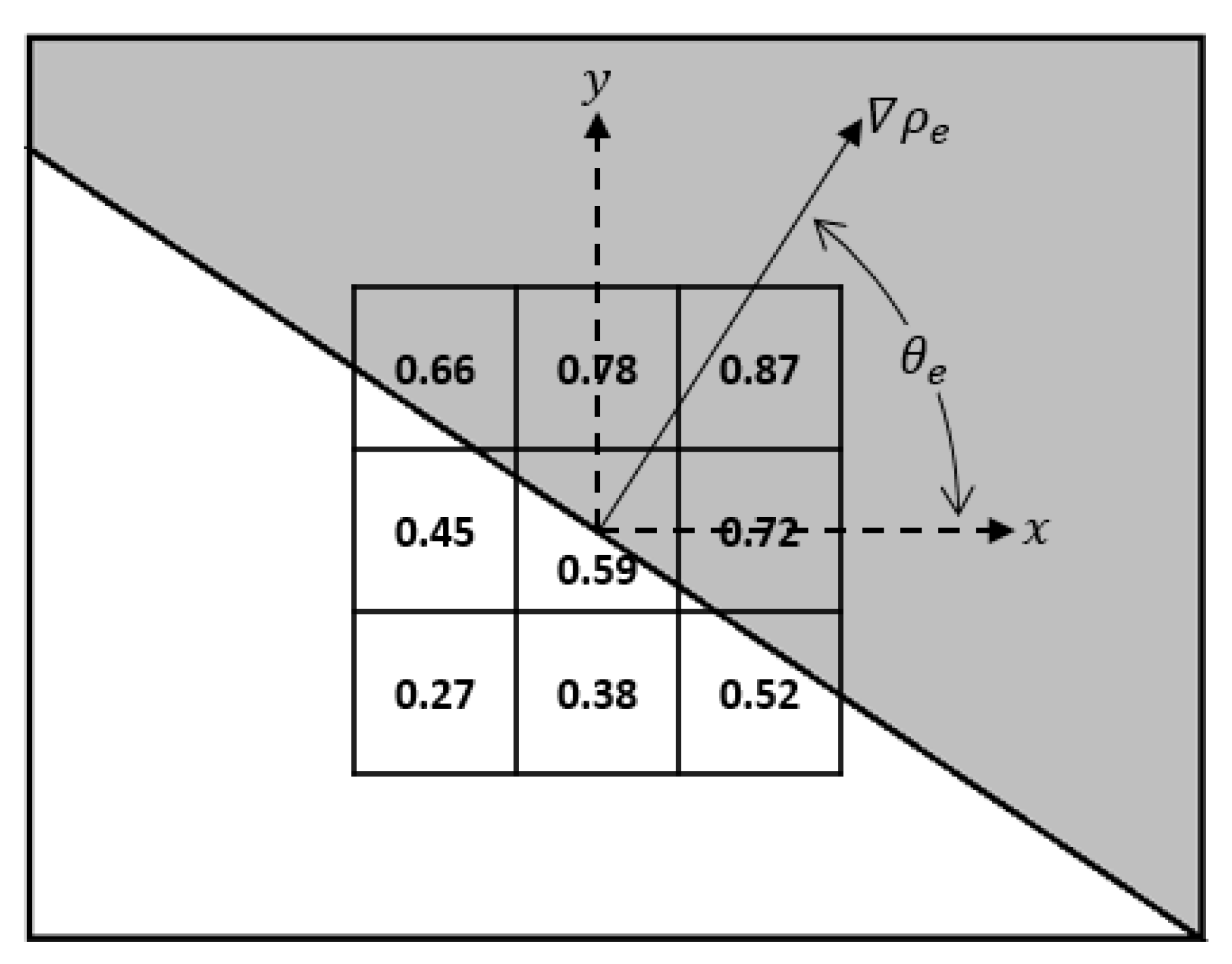
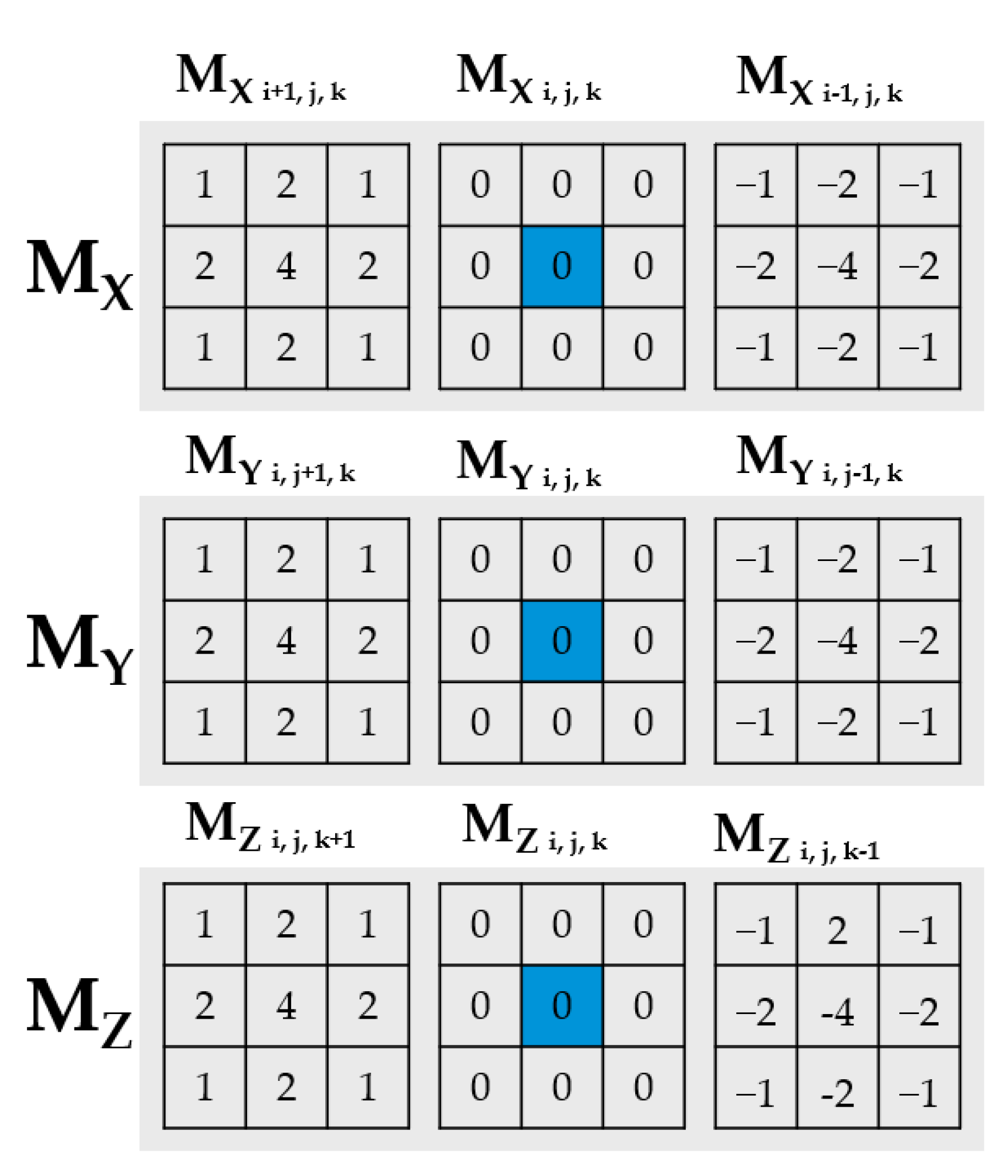
2.2. Two-Dimensional Density Gradient

In image processing, image points of high contrast (high magnitude of pixel intensity gradient) can be detected by computing the intensity differences in local image regions, which typically form the border between different objects in the scene. This process produces the magnitude and direction of contrast or gradient vector of the greyscale image pixel intensities. The magnitude of the contrast is typically applied in image processing for its ability to detect edges [29]. Note that the pixel intensities of a greyscale image are analogous to the elemental density matrix of a density-based topology optimization, where the intensity of an image pixel can be represented as a number between zero and one (dark and light) and an element’s relative density is represented as a number between zero and one (void and solid). This suggests that the direction of the gradient vector produced by the image processing difference operators can be used to determine the direction of the density gradient vector at the surface elements of the structure. A visual representation of the elemental density gradient vector can be seen in Figure 3.
The gradient vector is found using neighborhood templates, which are commonly referred to as masks or kernels, namely the masks known as Prewitt, Sobel, or Roberts masks [29]. The Prewitt mask is the basic form of the difference operator, as shown in Figure 4. This mask is sufficient for finding the gradient vector, although the results are noisy, meaning that the results produced may be significantly off from the true value. To help suppress this generated noise, the Prewitt mask is combined with a Gaussian filtering scheme and then referred to as the Sobel gradient mask.
In image processing, a mask approximating a Gaussian is used on its own as an image filter to remove “salt and pepper noise”. A Gaussian averaging mask was proposed and successfully implemented in [36] as an alternate filtering scheme for mesh-independent and checkerboard-free solutions, which demonstrates the applicability of image processing techniques to density-based topology optimization. Incorporating the Gaussian filtering into the Prewitt difference operators provides the advantage of weighting elements smoothly with the distance from the mask origin, meaning that the elemental density values nearer the central location are more important than the values that are more remote.
Mathematically, the density gradient vector, ρ e , is conveniently represented in the polar form by its magnitude and direction, denoted as:
ρ e = ρ e   ,   θ e  
The magnitude and direction of the gradient vector are calculated using the Cartesian components of the vector.
ρ e = ρ e x 2 + ρ e y 2  
θ e = t a n 1   ρ e y ρ e x  
where the Cartesian components of the elemental density gradient vectors, ρ e y and ρ e x , are calculated by convoluting the gradient masks to the density matrix. A detailed explanation of matrix convolution can be found in [29]. If there is not any gradient of the density in the x-direction, the denominator of Equation (8) will evaluate to zero, which should be taken into consideration during implementation. In this scenario, the gradient vector is either pointing straight up or straight down (±90°), and it can be determined by simply looking at whether the y-component of the gradient vector is positive (+90°) or negative (−90°). The Cartesian components of the gradient vector are determined using the matrix convolution between the density field and the Sobel or Prewitt gradient masks as follows:
ρ X = ρ × M x  
ρ Y = ρ × M y  
A sample elemental density and its eight-neighborhood are shown in the matrix of Figure 5. The density gradient vector points in the direction of the maximum increasing density visualized as the grey area in the figure, where, respectively, the grey/white areas represent the interpreted structure/void regions of the continuous design domain, which is represented by the 3 × 3 number matrix.

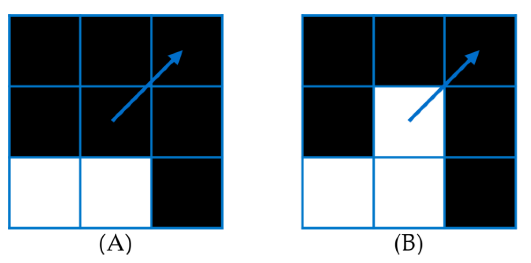
2.3. Limitations of the Gradient Vector’s Ability to Approximate Overhanging Angles

As explained in detail in the master’s thesis of Driessen [24], there exists some fundamental limitations in using the image processing method of the Prewitt and Sobel kernels convoluted to the density field to approximate the density gradients. Some configurations are shown in Figure 6, which shows that the approximated density gradient vector (blue arrow) does not point orthogonal to the surface (black elements). This occurs because the masks are approximating the gradient vector using a 3 × 3 kernel, which interprets a heavier concentration of material to one side of the element over the other. As the kernels become bigger, the number of elements that are misinterpreted also increases, which means a smaller kernel is more desirable for accurately approximating the true overhanging angle of a particular element. This limitation of misrepresented overhanging angles via the density gradient approximation is not a big concern when estimating support structure requirements because these misrepresentation occur one element at a time, which means that if the neighboring element is not self-supporting, then it will be identified as a region needing a support and small overhangs can occur next to a supported surfaces with minimal warping.

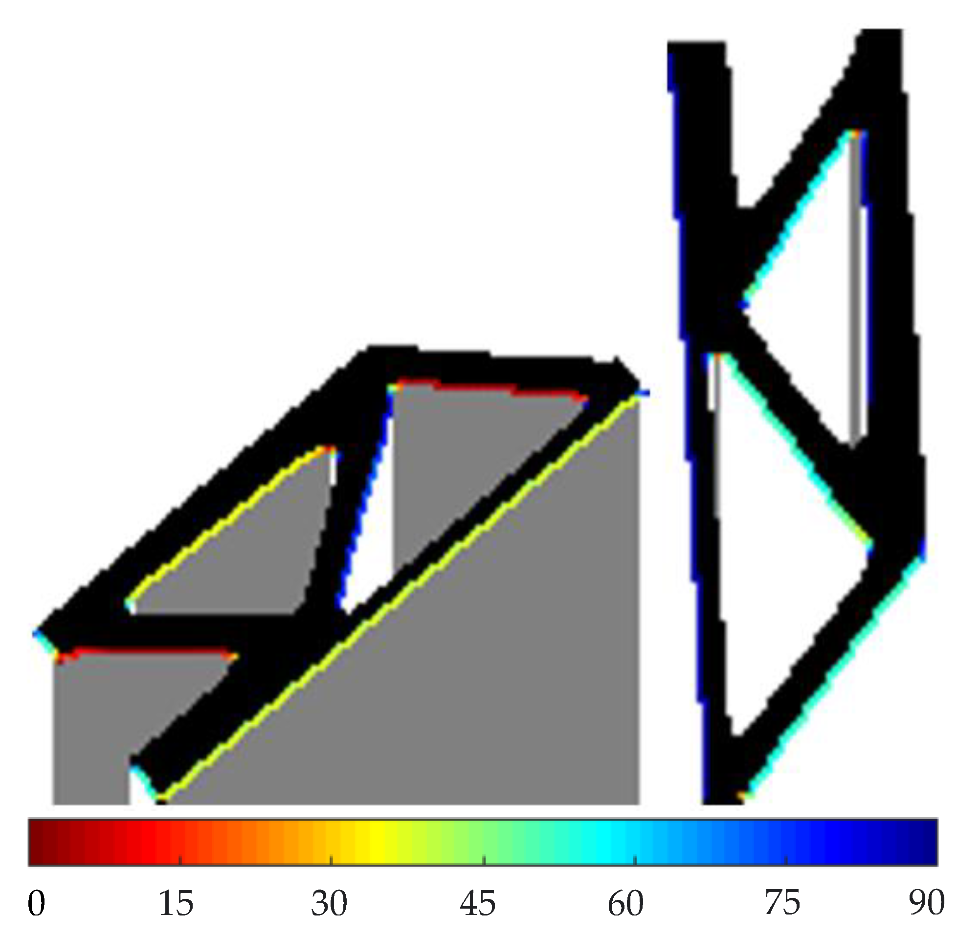
2.4. Support Slimming

As mentioned in Section 1, the overhanging surfaces of an additively manufactured part may require additional supporting structure to be printed, in addition to the part itself. The angle of an overhanging surface relative to the build platform is the main consideration when determining the proper locations for a supporting structure. As the angle of the overhanging surface decreases relative to the build platform, the ability of the structure to support itself as the material is being deposited decreases. This is true for most printing techniques, including the prevalent forms (i.e., FDM, SLS/DMLS, SLA). Typically, an overhanging surface with an angle of 45° or greater relative to the build platform is considered to be self-supporting. However, this is just a rule of thumb, and the actual self-supporting limit is not only process- and machine-dependent but also depends on the particular print settings, such as the laser scanning speed of a DMLS print. Liu et al. [37] state that from their in-house data, anywhere from 40% to 70% of the cost of producing an AM product could be avoided by removing the need for a support structure. The promise of cutting the cost of producing AM parts by half or more is the motivation for reducing the amount of required supporting structure (support slimming).
Support slimming has been extensively studied in recent years as the popularity of AM in both academia and industry has increased. The geometry of the supporting structure (i.e., tree-like, lattice, repetitive cellular structures, bridge-like scaffolding) plays a role in reducing the volume and/or associated costs of the supporting structure, although it is not the focus of this research. Support slimming is achieved by means of part orientation optimization based solely on the overhanging angle to demonstrate the applicability of the density gradient vector. As a part is reoriented relative to the build direction of an AM process, the angle of the overhanging surfaces relative to the build platform varies and, therefore, an orientation that minimizes the volume of supporting structure may be found.
Part orientation optimization has been studied on the STL representation of the structure [38,39]. The angle of an overhanging facet (STL representation of a surface) may simply be calculated by finding the angle of the facet’s normal vector relative to the build platform. Then, this information is used to calculate the volume of the region below un-supported overhanging surfaces. Bender and Barari [28] achieved part orientation optimization by calculating the overhanging surface angles using well-established image processing techniques to approximate the gradient of the density, which resulted from a density-based topology optimization. This technique was limited to two-dimensional problems, and the purpose of this research is to extend the image processing-based developed concept to three dimensions. This will allow us to solve the part orientation problem in the topology optimization of 3D cases. The results of part orientation optimization, which minimize and maximize the required supporting material using the density gradient information, can be visualized in Figure 7. The black area represents the topology-optimized structure, the colored areas represent elements on the perimeter of the structure that are overhanging, and the color spectrum represents the angles of the overhanging surfaces relative to the build platform.

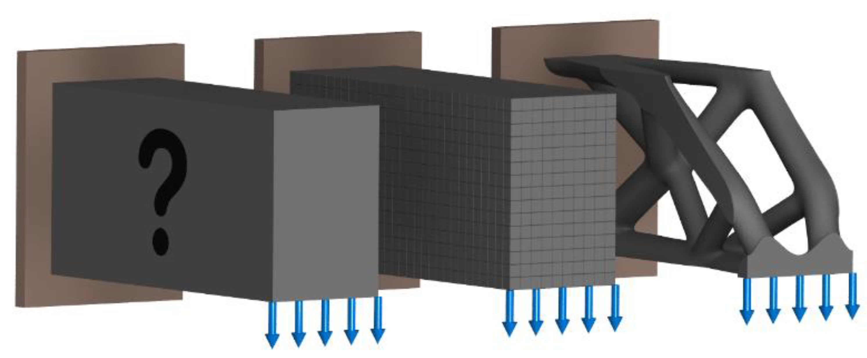
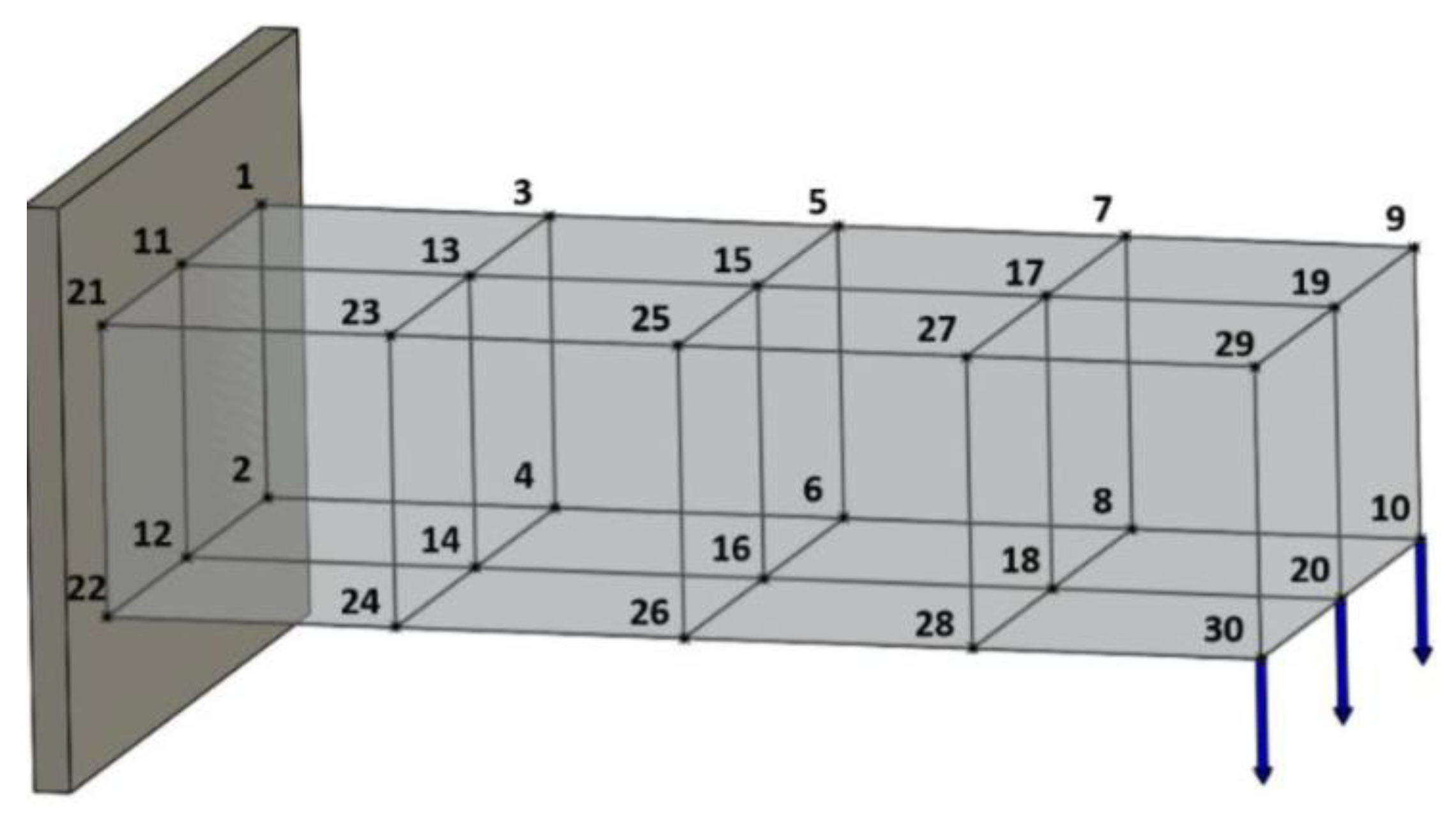
3. Developed Methodology

Referring to Figure 5, the Cartesian components of the elemental gradient, ρ e x and ρ e y , are respectively calculated across the local x- and y-axes. With only the 2 axes, the gradient components are simply calculated across a line. However, in order to calculate the gradient components in three dimensions, the three Cartesian components of the gradient must be calculated across their corresponding plane (the normal plane). Analogously to the image processing representation of a gradient component mask consisting of a 3 × 3 matrix of weights (Figure 4), the mask for calculating a 3D gradient component is a 3 × 3 × 3 matrix of weights. For easy representation, this matrix may be split up into 3 of these 3 × 3 matrices, as shown in Figure 8.
The masks in Figure 7 are similar in nature to the Prewitt image processing masks, such that they simply approximate the magnitude of the gradient across a plane. However, it is shown in [29] that additionally weighting the elements of the masks based on their distance from the central element helps to reduce noise, which in turn provides an approximation that is truer to the actual value. A mask resembling the less noisy Sobel equivalent is created by weighting the elements of the masks according to the distance, d , from the central element. The Gaussian distribution is implemented to generate distance-based weights. The equations of the Gaussian are:
g d = 1 2 π σ e d 2 2 σ 2  
and
g d = e d 2 2 σ 2  
where g d is the Gaussian weight with respect to the distance, d , between elements and σ controls how heavily weighted the elements further away from the central element are, which is also known as the spread of the distribution. Since the calculated magnitude of the gradient is divided by the sum of the weights of the mask (part of the matrix convolution process), the 1 2 π term of Equation (11) may be omitted to produce Equation (12). Equation (12) will generate weights with values between one and zero, which are multiplied by a constant to become integer values that are easier to display as a mask. The weights of the mask in Figure 8 are multiplied by the weights generated by Equation (12) to produce the derived masks needed to approximate the gradient of the density matrix. The product of these weights is shown in the masks in Figure 9.
Considering the representation of the gradient vector from Equation (6), the magnitude of the three-dimensional gradient vector in the polar form is calculated as:
ρ e = ρ e x 2 + ρ e y 2 + ρ e z 2  
Assuming that the build platform of a 3D printer is formed by the lowest XZ-plane of the design domain, the angle of the elemental gradient vector with respect to this plane may be calculated as described by Equation (14). It is possible for the denominator of this equation to evaluate to zero if there is no density gradient in the x- or z-direction. In this scenario, the magnitude along the y-direction can be solely looked at. If the magnitude is positive, the gradient vector is +90° measured from the build platform’s normal vector, while if the magnitude is negative, the gradient vector is −90°.
θ e = c o s 1 ρ e x 2 + ρ e z 2 ρ e x 2 + ρ e z 2       ρ e x 2 + ρ e y 2 + ρ e z 2  
More generally, the angle may be calculated using the dot product between the elemental gradient vector, ρ e = ρ e x   ρ e y   ρ e z , and the normal vector, n = n x   n y   n z , of the build platform.
θ e = c o s 1 ρ e ρ e   ·   n n  
Similar to Equations (9) and (10), the Cartesian components of the elemental gradient vectors are calculated via matrix convolution with the masks in Figure 9 with the density matrix.
ρ X = ρ × M X i + 1 , j , k + ρ × M X i , j , k + ρ × M X i 1 , j , k  
ρ Y = ρ × M Y i , j + 1 , k + ρ × M Y i , j , k + ρ × M Y i , j 1 , k
ρ Z = ρ × M Z i , j , k + 1 + ρ × M Z i , j , k + ρ × M Z i , j , k 1
where ρ represents the density matrix. It is worth noting that the middle terms in Equations (16)–(18), that is, the terms containing M X i , j , k , M Y i , j , k , and M Z i , j , k , may be omitted from the calculations since their masks contain only weights of zero value.
Using the methods described in this section, a three-dimensional structure resulting from topology optimization may be analyzed to allow for its supporting structure requirements to be additively manufactured. These locations are determined based on whether an overhanging surface angle relative to an AM build platform is below a self-supporting threshold or not. These overhanging surface angles are visualized in Figure 10.

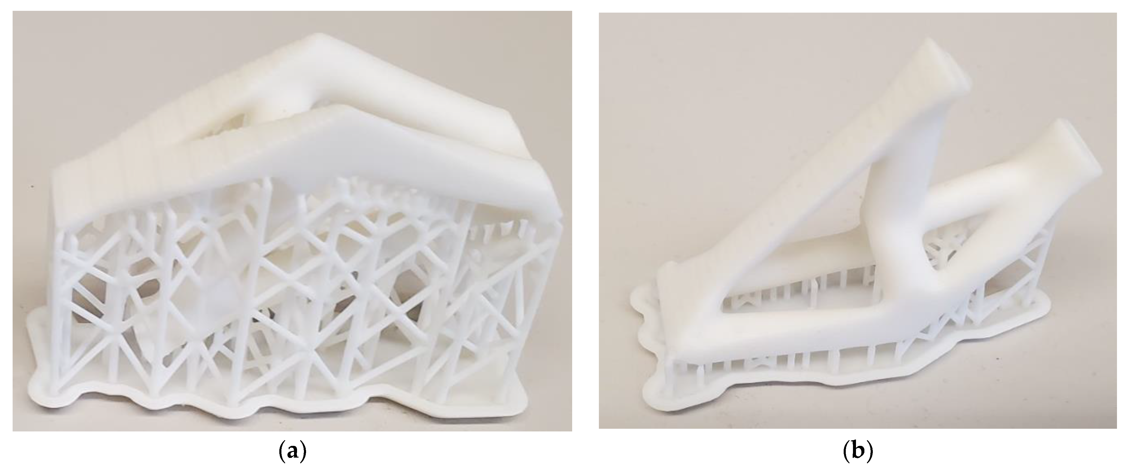
4. Implementation and Results

A direct application of the developed methodology in the estimation of the density gradient is to calculate the Required Support Volume (RSV) for a certain build orientation. This section presents the implementation results of the RSV calculation and a selection of best build orientations that minimize the RSV.
The analysis of the developed algorithms is carried out on three structural design problems, as seen in Table 1. The first problem is a benchmark problem often referred to as a “Mitchell structure” or “3D Wheel”. This structure is particularly chosen because of its two planes of symmetry. Its structure was topologically optimized using the code provided in the appendix of [30], with a total of 171,500 discrete elements comprising its finite mesh. The second structure is the standard cantilever benchmark problem consisting of 211,050 finite elements and 1 plane of symmetry. The last structure analyzed is a non-benchmark problem consisting of 171,500 finite elements with no spatial symmetry. The second and third structures were topologically optimized using the built-in feature of ANSYS™ 18.2. The density matrix of the final result was exported from ANSYS following processing and imputed into the implemented program in MATLAB™ for the custom overhanging feature analysis and support slimming analysis.
The first step in the analysis process is to analyze the overhanging surface angles and determine the locations of the surfaces that are not self-supported during 3D printing. This is performed by performing the matrix convolution of the density matrix in accordance with Equations (16)–(18) and the masks in Figure 8. Equation (14) is then applied to calculate the angle of the overhanging surfaces with respect to the build platform of an arbitrary 3D printer. If the angle is below a prescribed self-supporting angle, which is taken to be 45°, then the surface is considered to need a supporting structure. The total volume contained under the unsupported surfaces is calculated in the same manner as outlined in [28]. This entire analysis is carried out on the structure at rotations about the x- and y-axes between 0° and 360° to determine the orientations that minimize and maximize the supporting structure volume in a brute force manner.
The orientation optimization landscapes are presented in Table 1, while the results of the orientations that minimize and maximize the support structure volume are presented in Table 2. The smoothed isosurface visualization of the structure orientations that minimize the supporting structure volume is also presented in Table 2.
In order to also validate the results of the analytical solutions with actual experiments, the three topologically optimized parts were fabricated with the original and the optimized build orientations. The RSV for each case was measured by weighing the parts before and after removing the support structures. The RSV for the original build direction compared to the RSV for the optimum build direction is presented as a percentage in Table 3 for the theoretical and experiments studies.
As can be seen in Table 3, the differences between the experimental and analytical results are negligible. It is worth mentioning that the support structures in the fabricated parts are done in patterns, as defined by the utilized 3D printing software, and they are not meant to fill the entire RSV. This could potentially cause some differences between the theoretical and experimental RSV results. However, this difference has been negligible for all case studies (less than 2%). Figure 11 presents the images of the fabricated samples for the topologically optimized cantilever beam as examples. These samples were printed with general purpose resin on a Formlabs Form 2 SLA Printer.
The algorithm is implemented in MATLAB. The elemental density gradient vectors, angle analysis, and total support structure volume can be calculated relatively fast with the visual generation comparing the time required for the iterations in the topology optimization process. Comparatively, one iteration of the topology optimization process may take upwards of an hour to compute. All the analyses were carried out on an Intel Core i5-5300U, 2.30 GHz with 8 GB RAM.
It is worth noting that if there exists a plane of symmetry in the structural design, then there will be an axis of symmetry in the part orientation optimization landscape. This is evident in Table 1, where the first structure has two planes of symmetry and its corresponding optimization landscape has two axes of symmetry. This can also be seen in the second example in Table 1, where the structure has one plane of symmetry and its corresponding optimization landscape has one axis of symmetry. This is useful for reducing the time needed to optimize the parts orientation, as searching redundant optimization domains is time consuming.

5. Replication of the Results

A customized MATLAB script used to calculate the 3D density gradient vectors has been included in Appendix A, which may simply be adapted into the benchmark 3D topology optimization code provided in Appendix C of [34]. To approximate the density gradient vector, simply add this line of code after line 90 of the aforementioned topology optimization code:
91 [magnitude, direction] = DensityGradient(x);
The code provided in Appendix A should be included as either an auxiliary function to your script or as a standalone script contained within the working directory of your program. The function will return two matrices of the same size as the x matrix, one containing the magnitude of the elemental density gradient vector and the other the angle of the vector measured from the XZ-plane (assumed to be a build platform).
To visualize the results, the display_3D function can be simply modified to display the direction of the density gradient vector using a color map, such as the jet color scheme, to plot the elements instead of plotting them as a greyscale visualization of the densities similar to in Figure 9.

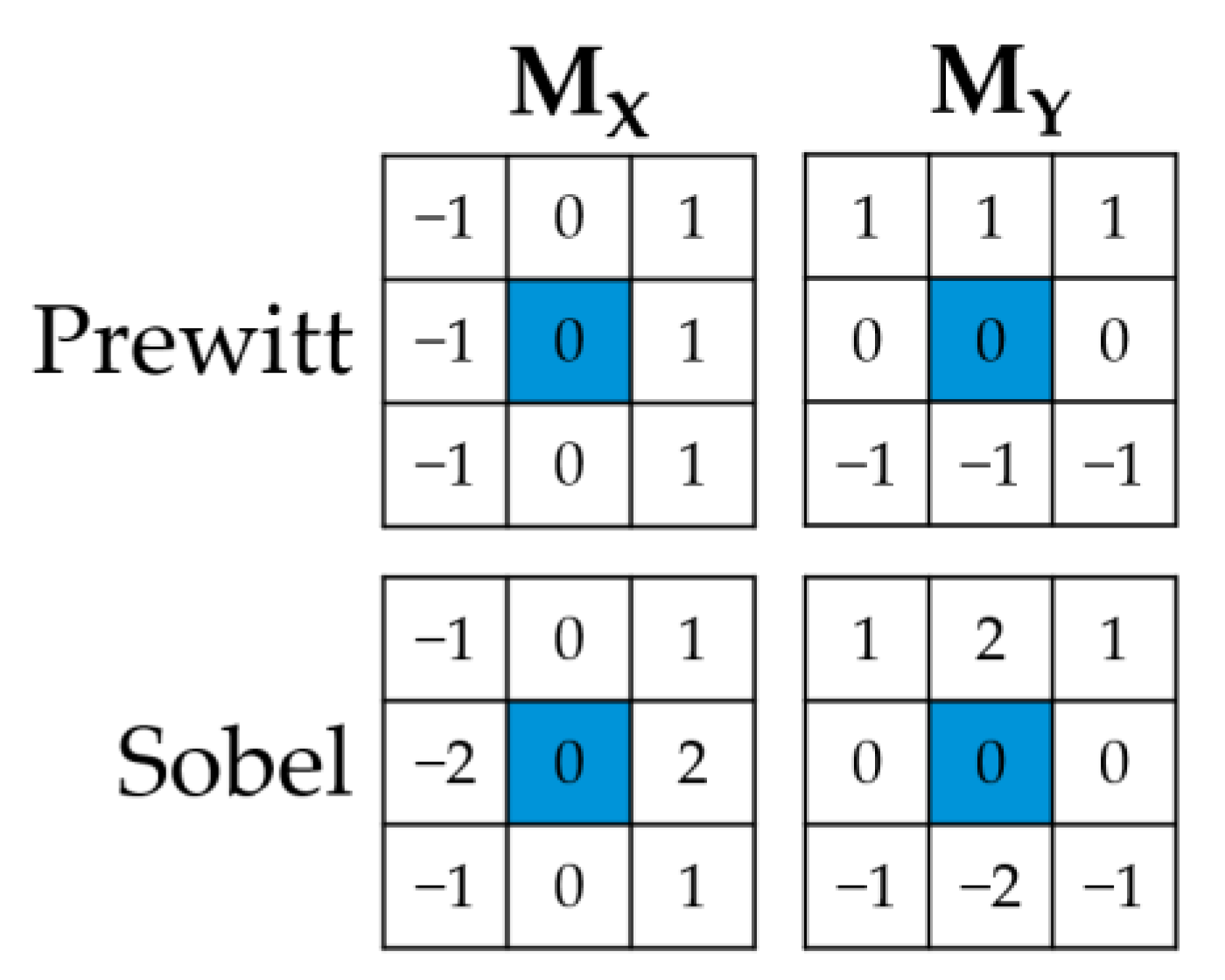
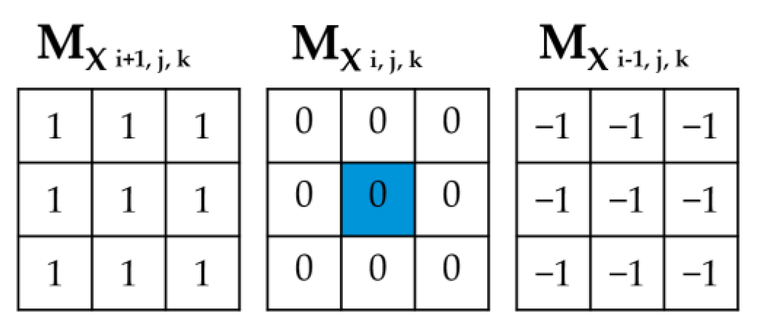
6. Filter Approach for Density Gradient Vectors

The methods presented in this article thus far are concerned with topology optimizations whose design domains consist of only squares (in 2D) and cubes (in 3D), although most practical applications decompose the design domain into multiple types of finite elements. A reconstruction of the computer vision derivation to form the masks of the previous sections is performed to achieve a continuous form of density gradient analysis based on the SIMP mesh independence filtering.
An approximation of the Cartesian components of the density gradient analysis is presented in Equations (19)–(21). The familiar SIMP filtering scheme is used with some minor changes. First, the filter is split into three components to analyze the gradient in the x-, the y-, and the z- directions individually with an additional directionality term added (dij|dij|), where dijx is the x-component of the distance between elements i and j. These functions essentially perform the exact same operations as the matrix convolution.
ρ e x = 1 j = 1 N G i j j = 1 N G i j ρ j d i j x d i j x  
ρ e y = 1 j = 1 N G i j j = 1 N G i j ρ j d i j y d i j y  
ρ e z = 1 j = 1 N G i j j = 1 N G i j ρ j d i j z d i j z  
The Gaussian weight factor (Gij) is used to smooth the results. It is recommended that the Gaussian weight factor is used for the purpose of noise reduction to achieve accurate approximations. The proposed weight factor for this filter is as follows:
G i j = 1 σ 2 π e d i j 2 2 σ 2  
This Gaussian weight factor has a component known as the spread factor (σ). It is recommended that this factor reflects the length scale used in the topology optimization process so that the local gradient analysis does not encompass multiple members and to ensure that the surface in question is adequately analyzed. It is recommended that the spread factor is taken as a third of the filter radius used in the SIMP optimization.
σ = r m i n 3  

7. Conclusions

This article presents a methodology for evaluating the three-dimensional gradient vector of the design domain in the topology optimization process. It also shows how the information of the three-dimensional gradient vector is used to analyze the overhanging surfaces of AM parts for purposes such as finding the optimum built orientation. This was achieved by extending the techniques from 2D image processing into 3D as well as by modifying a pre-existing topology optimization filter to achieve the same results as the image processing techniques. The developed algorithm is fully implemented, and a variety of experiments are conducted for validation purposes. The developed support slimming algorithm can be combined with any topology optimization process to consider the manufacturing requirement as an optimization constraint. Without losing generality, the developed methodology is implemented in combination with a SIMP-based topology optimization in this article. The results show that the presented technique for approximating the elemental density gradient vectors is an effective way to determine whether an overhanging surface requires a supporting structure to be effectively additively manufactured. Future works include extending the implementation of the developed approach to the overhanging surface analysis for different types of printing processes, materials, and support structure types to develop a complete understanding of the limitations of the overhanging surface of topology-optimized structures via density gradient vectors.

Author Contributions

Conceptualization, A.B.; methodology, D.B. and A.B.; soft-ware, D.B. and A.B.; validation, D.B.; formal analysis, D.B.; investigation, D.B. and A.B.; resources, A.B.; data curation, D.B.; writing—original draft preparation, D.B.; writing—review and editing, D.B. and A.B.; visualization, D.B.; supervision, A.B.; project administration, A.B.; funding acquisition, A.B. All authors have read and agreed to the published version of the manuscript.

Funding

Authors wish to acknowledge the funding and support received from the Natural Sciences and Engineering Research Council of Canada (NSERC).

Data Availability Statement

Original MATLAB code has been made available in the Appendix A. An explanation of its implementation into other publicly available MATLAB code is described in Section 5.

Conflicts of Interest

The authors declare no conflict of interest.

Appendix A. MATLAB Program Density Gradient

Jmmp 07 00046 i016Jmmp 07 00046 i017

References

  1. Huang, X.; Xie, M. Evolutionary Topology Optimization of Continuum Structures: Methods and Applications; John Wiley & Sons: Hoboken, NJ, USA, 2010. [Google Scholar]
  2. Sigmund, O.; Maute, K. Topology optimization approaches. Struct. Multidisc. Optim. 2013, 48, 1031–1055. [Google Scholar] [CrossRef]
  3. Atzeni, E.; Iuliano, L.; Marchiandi, G.; Minetola, P.; Salmi, A.; Bassoli, E.; Denti, L.; Gatto, A. Additive manufacturing as a cost-effective way to produce metal parts. In High Value Manufacturing: Advanced Research in Virtual and Rapid Prototyping, Proceedings of the 6th International Conference on Advanced Research and Rapid Prototyping, VR@ P, Leiria, Portugal, 1–5 October 2013; CRC Press, Inc.: Boca Raton, FL, USA, 2014; Volume 2013, pp. 3–8. [Google Scholar]
  4. Ngo, T.D.; Kashani, A.; Imbalzano, G.; Nguyen, K.T.; Hui, D. Additive manufacturing (3D printing): A review of materials, methods, applications and challenges. Compos. Part B Eng. 2018, 143, 172–196. [Google Scholar] [CrossRef]
  5. Marchesi, T.R.; Laherta, R.D.; Silva, E.C.N.; Tsuzuki, M.D.S.G.; Martins, T.D.C.; Barari, A.; Wood, I. Topologically optimized diesel engine support manufactured with additive manufacturing. In IFAC Symposium on Information Control Problems in Manufacturing; Elsevier: Bergamo, Italy, 2018. [Google Scholar]
  6. Doubrovski, Z.; Verlinden, J.C.; Geraedts, J.M. Optimal design for additive manufacturing: Opportunities and challenges. In Proceedings of the ASME 2011 International Design Engineering Technical Conferences and Computers and Information in Engineering Conference, Washington, DC, USA, 28–31 August 2011; American Society of Mechanical Engineers: New York, NY, USA, 2011; pp. 635–646. [Google Scholar]
  7. Brackett, D.; Ashcroft, I.; Hague, R. Topology optimization for additive manufacturing. In Proceedings of the Solid Freeform Fabrication Symposium, Austin, TX, USA, 8–10 August 2011; Volume 1, pp. 348–362. [Google Scholar]
  8. Lalehpour, A.; Barari, A. Post processing for Fused Deposition Modeling Parts with Acetone Vapour Bath. IFAC-PapersOnLine 2016, 49, 42–48. [Google Scholar] [CrossRef]
  9. Lalehpour, A.; Barari, A. A more accurate analytical formulation of surface roughness in layer-based additive manufacturing to enhance the product’s precision. Int. J. Adv. Manuf. Technol. 2018, 96, 3793–3804. [Google Scholar] [CrossRef]
  10. Sikder, S.; Barari, A.; Kishawy, H.A. Effect of adaptive slicing on surface integrity in additive manufacturing. In Proceedings of the ASME 2014 International Design Engineering Technical Conferences and Computers and Information in Engineering Conference, Buffalo, NY, USA, 17–20 August 2014; American Society of Mechanical Engineers: New York, NY, USA, 2014; p. V01AT02A052. [Google Scholar]
  11. Sikder, S.; Barari, A.; Kishawy, H.A. Global adaptive slicing of NURBS based sculptured surface for minimum texture error in rapid prototyping. Rapid Prototyp. J. 2015, 21, 649–661. [Google Scholar] [CrossRef]
  12. Gohari, H.; Kishawy, H.; Barari, A. Adaptive variable layer thickness and perimetral offset planning for layer-based additive manufacturing processes. Int. J. Comput. Integr. Manuf. 2021, 34, 964–974. [Google Scholar] [CrossRef]
  13. Di Angelo, L.; Di Stefano, P.; Guardiani, E. Search for the Optimal Build Direction in Additive Manufacturing Technologies: A Review. J. Manuf. Mater. Process. 2020, 4, 71. [Google Scholar] [CrossRef]
  14. Bendsøe, M.P. Optimal shape design as a material distribution problem. Struct. Optim. 1989, 1, 193–202. [Google Scholar] [CrossRef]
  15. Bendøse, M.P.; Sigmund, O. Topology Optimization: Theory, Methods and Applications; Springer: Berlin/Heidelberg, Germany, 2003; ISBN 3-540-42992-1. [Google Scholar]
  16. Barari, A.; ElMaraghy, H.A.; Orban, P. NURBS representation of actual machined surfaces. Int. J. Comput. Integr. Manuf. 2009, 22, 395–410. [Google Scholar] [CrossRef]
  17. Barari, A.; ElMaraghy, H.A.; Knopf, G.K. Evaluation of geometric deviations in sculptured surfaces using probability density estimation. In Models for Computer Aided Tolerancing in Design and Manufacturing: Selected Conference Papers from the 9th CIRP International Seminar on Computer-Aided Tolerancing; Springer Netherlands: Tempe, AZ, USA, 2007; pp. 135–146. [Google Scholar]
  18. Barari, A.; Mordo, S. Effect of sampling strategy on uncertainty and precision of flatness inspection studied by dynamic minimum deviation zone evaluation. Int. J. Metrol. Qual. Eng. 2013, 4, 3–8. [Google Scholar] [CrossRef]
  19. Gohari, H.; Berry, C.; Barari, A. A digital twin for integrated inspection system in digital manufacturing. IFAC-PapersOnLine 2019, 52, 182–187. [Google Scholar] [CrossRef]
  20. Wang, D.; Yang, Y.; Yi, Z.; Su, X. Research on the fabricating quality optimization of the overhanging surface in SLM process. Int. J. Adv. Manuf. Technol. 2013, 65, 1471–1484. [Google Scholar] [CrossRef]
  21. Calignano, F. Design optimization of supports for overhanging structures in aluminum and titanium alloys by selective laser melting. Mater. Des. 2014, 64, 203–213. [Google Scholar] [CrossRef]
  22. Zhu, J.; Zhou, H.; Wang, C.; Zhou, L.; Yuan, S.; Zhang, W. A review of topology optimization for additive manufacturing: Status and challenges. Chin. J. Aeronaut. 2021, 34, 91–110. [Google Scholar] [CrossRef]
  23. Leary, M.; Merli, L.; Torti, F.; Mazur, M.; Brandt, M. Optimal topology for additive manufacture: A method for enabling additive manufacture of support-free optimal structures. Mater. Des. 2014, 63, 678–690. [Google Scholar] [CrossRef]
  24. Driessen, A.M. Overhang Constraint in Topology Optimisation for Additive Manufacturing: A Density Gradient Based Approach; Delft University of Technology: Delft, The Netherlands, 2016. [Google Scholar]
  25. Garaigordobil, A.; Ansola, R.; Santamaría, J.; de Bustos, I.F. A new overhang constraint for topology optimization of self-supporting structures in additive manufacturing. Struct. Multidiscip. Optim. 2018, 58, 2003–2017. [Google Scholar] [CrossRef]
  26. Mass, Y.; Amir, O. Topology optimization for additive manufacturing: Accounting for overhang limitations using a virtual skeleton. Addit. Manuf. 2017, 18, 58–73. [Google Scholar] [CrossRef]
  27. Qian, X. Undercut and overhang angle control in topology optimization: A density gradient based integral approach. Int. J. Numer. Methods Eng. 2017, 111, 247–272. [Google Scholar] [CrossRef]
  28. Bender, D.; Barari, A. Overhanging Feature Analysis for the Additive Manufacturing of Topology Optimized Structures. In Proceedings of the ASME 2018 International Design Engineering Technical Conferences and Computers and Information in Engineering Conference, Quebec City, QC, Canada, 26–29 August 2018. [Google Scholar]
  29. Shapiro, L.G.; Stockman, G.C. Computer Vision; Pearson: London, UK, 2000. [Google Scholar]
  30. Jamiolahmadi, S.; Barari, A. Surface topography of additive manufacturing parts using a finite difference approach. J. Manuf. Sci. Eng. 2014, 136, 061009. [Google Scholar] [CrossRef]
  31. Gohari, H.; Barari, A.; Kishawy, H. Using Multistep Methods in Slicing 2 ½ Dimensional Parametric Surfaces for Additive Manufacturing Applications. IFAC-PapersOnLine 2016, 49, 67–72. [Google Scholar] [CrossRef]
  32. Gohari, H.; Barari, A.; Kishawy, H. An efficient methodology for slicing NURBS surfaces using multi-step methods. Int. J. Adv. Manuf. Technol. 2018, 95, 3111–3125. [Google Scholar] [CrossRef]
  33. Andreassen, E.; Clausen, A.; Schevenels, M.; Lazarov, B.S.; Sigmund, O. Efficient topology optimization in MATLAB using 88 lines of code. Struct. Multidisc. Optim. 2011, 43, 117–137. [Google Scholar] [CrossRef]
  34. Liu, K.; Tovar, A. An efficient 3D topology optimization code written in Matlab. Struct. Multidisc. Optim. 2014, 50, 1175–1196. [Google Scholar] [CrossRef]
  35. Rietz, A. Sufficiency of a finite exponent in SIMP (power law) methods. Struct. Multidisc. Optim. 2001, 21, 159–163. [Google Scholar] [CrossRef]
  36. Li, Q.; Steven, G.P.; Xie, Y.M. A simple checkerboard suppression algorithm for evolutionary structural optimization. Struct. Multidisc. Optim. 2001, 22, 230–239. [Google Scholar] [CrossRef]
  37. Liu, J.; Gaynor, A.T.; Chen, S.; Kang, Z.; Suresh, K.; Takezawa, A.; Li, L.; Kato, J.; Tang, J.; Wang, C.C.; et al. Current and future trends in topology optimization for additive manufacturing. Struct. Multidisc. Optim. 2018, 57, 2457–2483. [Google Scholar] [CrossRef]
  38. Muir, M.J.; Querin, O.M.; Toropov, V. Rules, Precursors and Parameterisation Methodologies for Topology Optimised Structural Designs Realised through Additive Manufacturing. In Proceedings of the 10th AIAA Multidisciplinary Design Optimization Conference, National Harbor, MD, USA, 13–17 January 2014; p. 0635. [Google Scholar]
  39. Morgan, H.D.; Cherry, J.A.; Jonnalagadda, S.; Ewing, D.; Sienz, J. Part orientation optimisation for the additive layer manufacture of metal components. Int. J. Adv. Manuf. Technol. 2016, 86, 1679–1687. [Google Scholar] [CrossRef] [Green Version]
  40. Bender, D. Integrated Topology Optimization Design and Process Planning for Additive Manufacturing; University of Ontario Institute of Technology: Oshawa, ON, Canada, 2019. [Google Scholar]
Figure 1. The process of structural design by means of topology optimization: (1) define the design problem; (2) discretize the design domain; and (3) optimize the structure’s topology to achieve an efficient design.
Jmmp 07 00046 g001
Figure 2. Global node IDs in a prismatic structure composed of 8 elements and 30 nodes.
Jmmp 07 00046 g002
Figure 3. The detail shows part of the density field with the approximated gradients of the density field. The gradient vectors point in the direction of increasing density [22].
Jmmp 07 00046 g003
Figure 4. Two examples of a pair of masks used to approximate the Cartesian components of an image’s intensity gradient.
Jmmp 07 00046 g004
Figure 5. A visualization of the elemental density gradient vector at an element.
Jmmp 07 00046 g005
Figure 6. Density configurations that are misinterpreted by the Sobel/Prewitt kernels.. Both subfigures (A) and (B) show that the density gradient approximation via matrix convolution is 45° rather than the naturally perceived overhanging angle of 90°.
Jmmp 07 00046 g006
Figure 7. Print orientations that maximize (left) and minimize (right) the required volume of supporting structure [40].
Jmmp 07 00046 g007
Figure 8. Masks that are used to approximate the gradient across the x-plane. These masks are akin to the 2D Prewitt masks for image processing.
Jmmp 07 00046 g008
Figure 9. Masks that are used to approximate the gradient across each of the cartesian planes. These masks are akin to the Sobel masks for image processing.
Jmmp 07 00046 g009
Figure 10. A sample overhanging surface angle analysis of a cantilever: (left) facets of the finite elements are colored and (right) a smoothed isosurface.
Jmmp 07 00046 g010
Figure 11. Examples of the fabricated samples for the experimental topologically optimized cantilever beam: (a) orientation with maximum required support volume; and (b) orientation with minimum required support volume.
Jmmp 07 00046 g011
Table 1. Three structural design problems, results of the topology optimization, and corresponding landscapes of the orientation optimization.
Structural Design Problem and the Resulting TopologyPart Orientation Optimization Landscape
Top. Opt. Software:

Nelx: 70
Nely: 35
Nelz: 70

Two planes of symmetry
Jmmp 07 00046 i001Jmmp 07 00046 i002
Top. Opt. Software:
ANSYS 18.2

Nelx: 45
Nely: 67
Nelz: 70

One plane of symmetry
Jmmp 07 00046 i003Jmmp 07 00046 i004
Top. Opt. Software:
ANSYS 18.2

Nelx: 70
Nely: 35
Nelz: 70

No symmetry
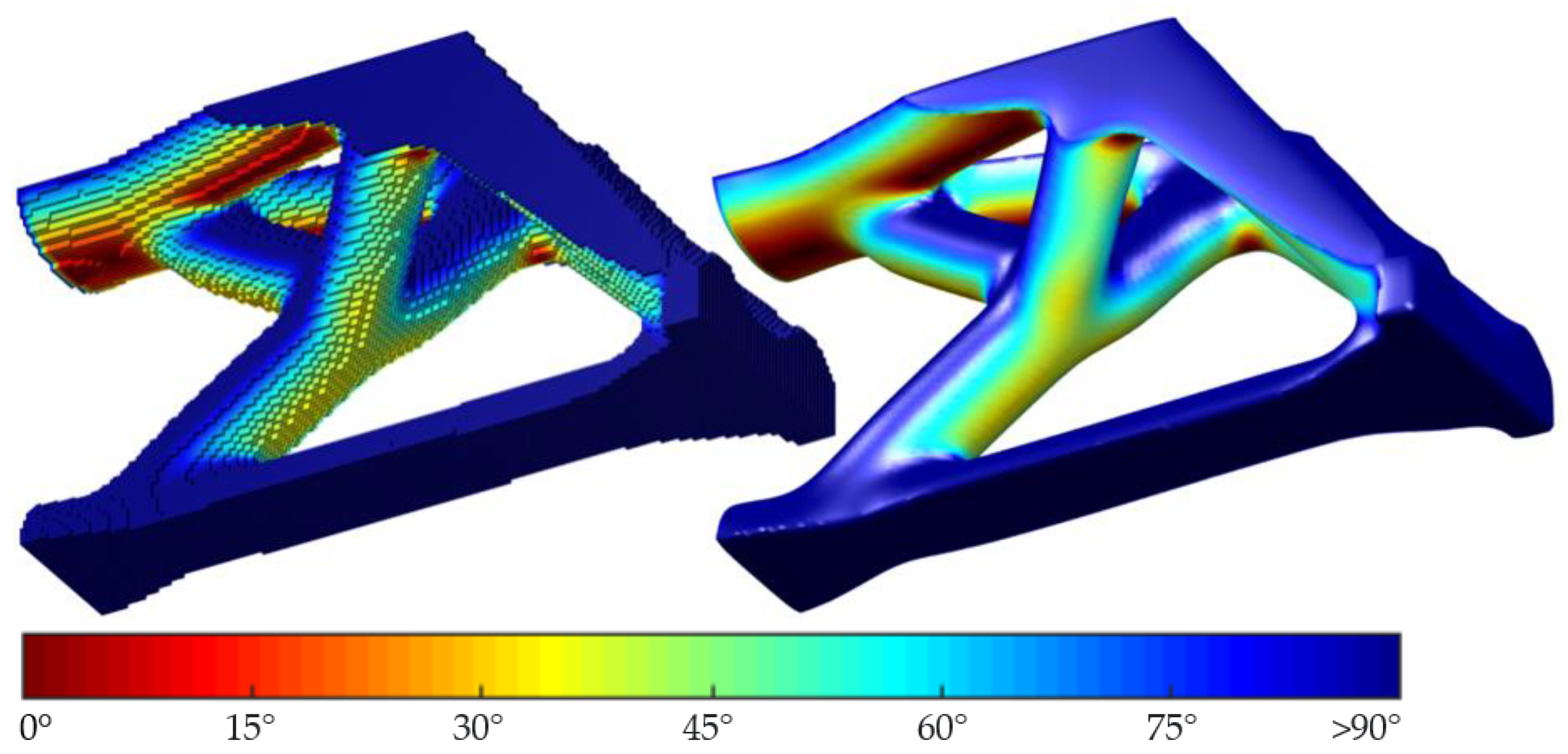
Jmmp 07 00046 i005Jmmp 07 00046 i006
Table 2. Part orientations that minimize and maximize the required support volume with surface angle visuals of the minimum orientation.
Minimum RSV OrientationMaximum RSV OrientationSurface Overhang Angle w.r.t the Build Platform Visualization @ min Support Orientation
Jmmp 07 00046 i007Jmmp 07 00046 i008Jmmp 07 00046 i009
Jmmp 07 00046 i010Jmmp 07 00046 i011Jmmp 07 00046 i012
Jmmp 07 00046 i013Jmmp 07 00046 i014Jmmp 07 00046 i015
Table 3. Comparing the experimental results with the maximum and minimum RSV calculated using the developed methodology.
Case StudyTheoretical Weight Difference between the Original Build Direction an Optimal Build DirectionExperimental Weight Difference between the Original Build Direction an Optimal Build DirectionDifference between Theoretical and Experimental Results
Michell174.32%171.35%1.7%
Cantilever170.70%169.8%0.5%
Asymmetric148.02%145.7%1.5%
Disclaimer/Publisher’s Note: The statements, opinions and data contained in all publications are solely those of the individual author(s) and contributor(s) and not of MDPI and/or the editor(s). MDPI and/or the editor(s) disclaim responsibility for any injury to people or property resulting from any ideas, methods, instructions or products referred to in the content.

