Mechanical Performance over Energy Expenditure in MEX 3D Printing of Polycarbonate: A Multiparametric Optimization with the Aid of Robust Experimental Design

Abstract

Sustainability and energy efficiency of additive manufacturing (AM) is an up-to-date industrial request. Likewise, the claim for 3D-printed parts with capable mechanical strength remains robust, especially for polymers that are considered high-performance ones, such as polycarbonates in material extrusion (MEX). This paper explains the impact of seven generic control parameters (raster deposition angle; orientation angle; layer thickness; infill density; nozzle temperature; bed temperature; and printing speed) on the energy consumption and compressive performance of PC in MEX AM. To meet this goal, a three-level L27 Taguchi experimental design was exploited. Each experimental run included five replicas (compressive specimens after the ASTM D695-02a standard), summating 135 experiments. The printing time and the power consumption were stopwatch-derived, whereas the compressive metrics were obtained by compressive tests. Layer thickness and infill density were ranked the first and second most significant factors in energy consumption. Additionally, the infill density and the orientation angle were proved as the most influential factors on the compressive strength. Lastly, quadratic regression model (QRM) equations for each response metric versus the seven control parameters were determined and evaluated. Hereby, the optimum compromise between energy efficiency and compressive strength is attainable, a tool holding excessive scientific and engineering worth.

1. Introduction

Sustainability is lately a key issue for all aspects of society (government, enterprises, and public) for both products and processes [1]. AM is considered a process with better sustainability characteristics compared to traditional manufacturing processes due to its energy consumption and reduced material waste [1,2]. Additionally, the sustainability aspects of AM are gaining attention in the literature since it has become one of the important tools facilitating the manufacturing of products [3,4]. The effect of environmental factors [5,6,7], the recycling of the materials [8,9], and the process parameters [10] on the sustainability of the AM process have been investigated. One of the factors affecting the sustainability of a process is energy consumption [11]. The energy efficiency of MEX polymer processing has been investigated in the literature [12]; however, research is not yet extensive. The energy demands in MEX 3D printing of high-performance polymers, such as PEEK, have been investigated with a full factorial design, considering two 3D printing parameters, i.e., layer thickness and printing speed [13]. Interpretive structural modeling (ISM) has also been employed for the analysis of parameters affecting energy consumption in MEX 3D printing [11]. The effect of parameters, such as the infill pattern, on energy consumption, has also been investigated [14] for materials such as the ABS polymer [15]. Energy consumption has also been studied using machine learning techniques [16]. The effect of six 3D printing parameters on the energy consumption of parts built by ABS polymer with the MEX 3D printing process has been analyzed and optimized with statistical modeling tools [17]. Energy modeling techniques have also been applied [18]. The effect of energy consumption on parameters such as the required 3D printing time [19] and geometric accuracy [20] has been studied.

PC is a high-performance polymer [21], with tensile strength higher than 62 MPa, even when recycled, and a glass transition of about 121 °C [22], which makes it suitable for applications requiring high strength and high thermal loadings [23]. Therefore, it is used in safety parts, such as bulletproof glass in automobiles, helmets, and bumpers, but also electronics in capacitors [21,24,25]. In composite form, it has been used in electromagnetic shielding [26,27] and in construction [28,29] to improve the resistance to fire of materials [30]. PC blends are popular in biomedical devices and aerospace parts [21,29,31] and exhibit high energy-absorbing properties [32]. In 3D printing, it has been applied in aeronautical [33] and biomedical applications [34,35,36]. Still, the use and the research on the PC polymer in AM, overall, are not so extensive. Its mechanical properties under tensile [37] and shear forces have been investigated [38,39]. The effect of 3D printing parameters on the mechanical response of parts made with the PC polymer under tensile loading has been reported. Statistical tools have been employed for the analysis and optimization of the results [40]. Such an approach, by employing modeling tools, statistical and regression analysis, or even neural networks for the analysis and optimization of the performance of the 3D-printed parts, is often used in the literature [41,42,43,44].

The effect of 3D printing parameters on the response of PC 3D-printed parts under different strain rates in tensile tests has also been reported [45], and the impact strength of such parts as well [46]. In MEX 3D printing, the mechanical performance of recycled PC polymer has been reported, promoting a sustainable character to the polymer [23]. Quality characteristics related to the dimensional accuracy of 3D-printed parts built with the PC polymer have been studied [47]. The mechanical properties of PC composites in 3D printing have been investigated for carbon-based composites [48,49], and nanocomposites with titanium carbide [50], aluminum nitride [51], titanium nitride [52], silicon carbide [53], silica [54], and cellulose nanofibers [55]. PC/ABS blends in 3D printing have also been presented aiming to enhance the mechanical properties and the printability of the materials [56,57,58,59].

For the analysis of the performance of the PC polymer in MEX 3D printing, statistical tools, such as the Taguchi experiment design, have been employed [40,47,60,61,62], along with simulation tools [63]. The PC polymer has also been applied in hybrid additive manufacturing processes to further expand its applicability. MEX 3D printing has been combined with friction stir welding for the production of large-size parts [64] and with CO₂ laser cutting processes for the improvement in surface quality characteristics [65]. The compressive strength of the PC polymer has been studied in the pure form [66], recycled form [23] in 3D printing [67,68], and specifically for aeronautical [33] and medical [34] applications. Additionally, the effect of strain rate on the compressive strength of 3D-printed parts has been reported [69]. Still, there is a gap in the literature in the thorough analysis of the effects of the MEX 3D printing parameters on the compression response of the PC polymer. Additionally, the energy demands when 3D printing PC parts with the MEX process have not yet been addressed in the literature, and especially a study is missing on how the energy requirements are affected by the 3D printing parameters.

In the current study, the effect of seven 3D printing parameters, i.e., raster deposition angle, orientation angle, layer thickness, infill density, nozzle temperature, bed temperature, and printing speed, on the energy consumption and the response under compressive loading of parts made of PC with MEX 3D printing is reported. The 3D printing settings were selected to be generic and machine independent. Ten metrics related to energy consumption, the compression properties, and the quality of the 3D printing parts are evaluated with statistical and regression modeling tools.

Despite the compressive specimens’ increased printing time, volume, and weight (when compared to tensile specimens), this work focused on this mechanical property for reasons explained further in the text. Compression test data in multi-parametric experiments are limited in the literature, probably due to the increased effort required for the preparation of the samples with the 3D printing process. Considering that the compressive loads are the most frequent in the functional 3D-printed parts life cycle [70], this shortfall of data is remarkable. The increased mass and volume of the compression test specimens facilitate the monitoring and documentation of parameters in this work, such as the printing time, weight, and energy consumption, leading to more accurate results. Additionally, data for the mechanical performance of the PC polymer in MEX 3D printing are overall limited in the literature.

Equations as functions of the 3D printing settings (control parameters) were compiled, and their reliability was verified with confirmation experiments. The energy-related metrics were monitored during the MEX 3D printing process. The PC polymer was extruded from raw material to filament form, and specimens were 3D printed with this filament to be tested for their performance under compressive load. For the preparation of the specimens and performing the compression tests, the ASTM D695-02a international standard was followed. We also examined 3D-printed specimens for their morphological characteristics before and after the compression experiments. To the authors’ best knowledge, no research so far simultaneously studies seven 3D printing parameters for their effect on energy consumption and the thorough analysis of the compressive behavior of PC MEX 3D-printed parts. The prediction models provide valuable information about the expected performance of the parts, indicating direct industrial merit. The statistical analysis showed that each parameter affects the metrics studied in this work differently, making the modeling procedure a requisite. Infill density was the dominant parameter regarding compression strength, while layer thickness was the dominant parameter regarding energy consumption.

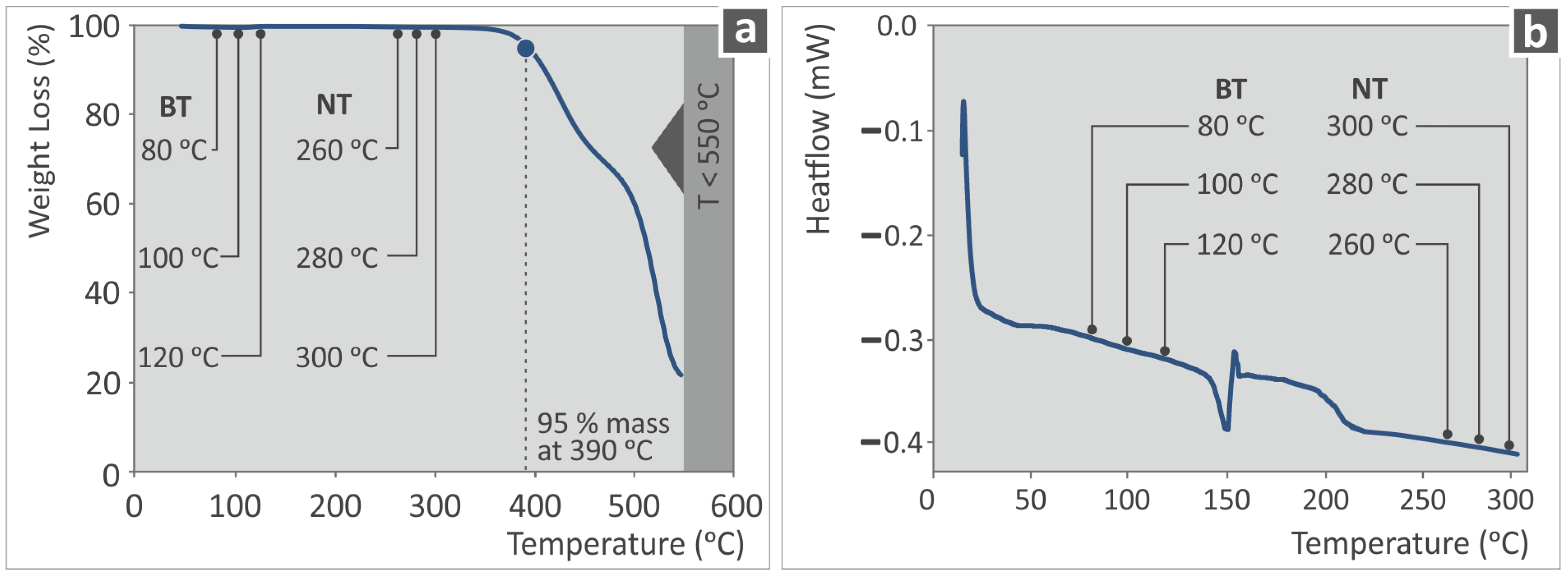
2. Materials and Methods

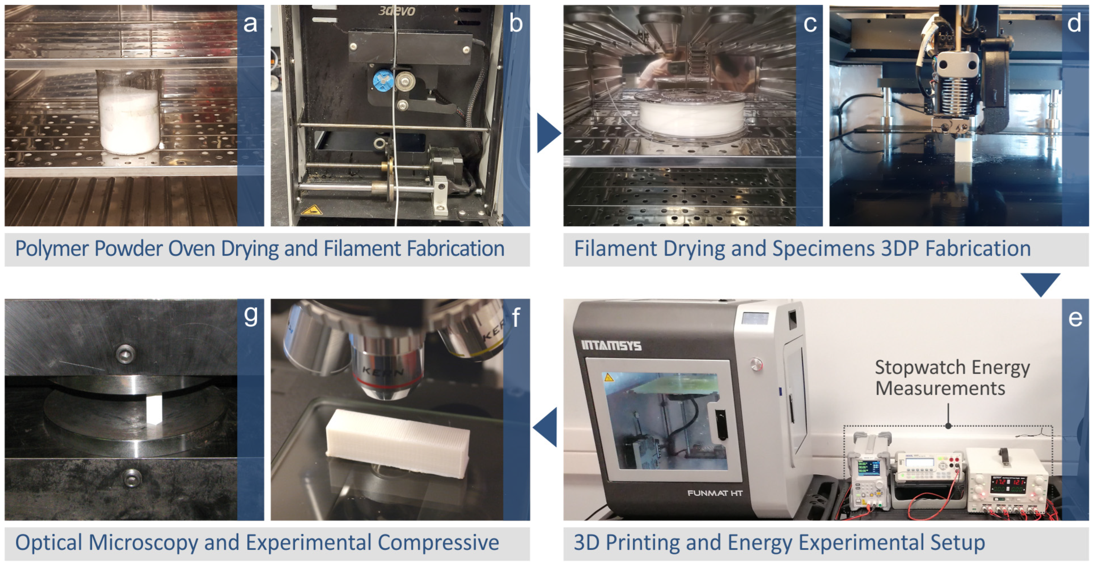
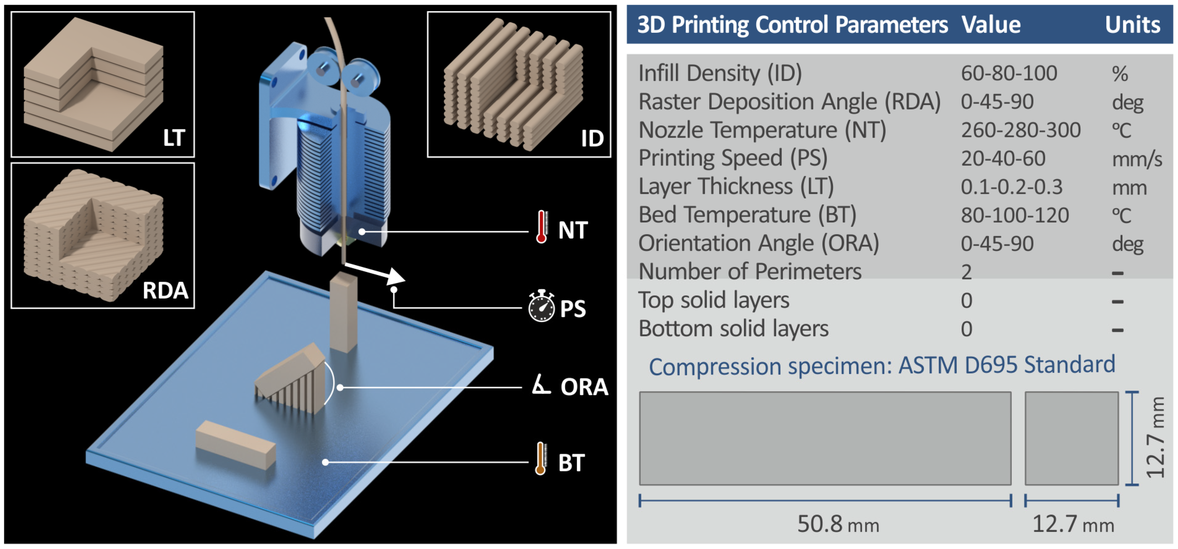
2.1. Methodology for Sample Preparation and Testing

Figure 1 presents snapshots of the steps followed in this work for the preparation of the samples and the experiments conducted. The PC polymer was sourced from Styron Europe GmbH (Trinseo Europe GmbH, Horgen, Switzerland) in pellet form (grade EMERGE 8430–15, a tensile strength of 70.0 MPa, and a density of 1.20 g/cm³). Pellets were initially dried (Figure 1a) for 14 h at 60 °C. Then a 3devo Precision (3devo, Utrecht, The Netherlands) MEX filament extruder was used for the production of 1.75 mm filament compatible with the MEX 3D printing process (Figure 1b, the first three heating zones operated at 200 °C, while the fourth heating zone operated at 240 °C, and screw speed was set at 4.8 rpm). The thermal properties of the specific PC grade were evaluated with TGA (Figure 2a) and DSC (Figure 2b) to ensure that the extrusion temperatures in this work do not cause any degradation in the PC polymer.

The produced filament was dried (Figure 1c, 60 °C for 4 h). All the filaments were produced, and then the 3D printing process followed, which was not conducted on the same day. After the production of the filament, it was not stored in a vacuum case or a laboratory oven, so it might have had moisture, as polymeric materials attract moisture easily. This moisture significantly affects the 3D printing process. So, in order to ensure that there was no humidity trapped in the filament before it was used in the 3D printing process, the filament was dried initially before being used in MEX 3D printing process.

With this filament, specimens were MEX 3D printed (Figure 1d) on an Intamsys, Funmat HT (Intamsys, Shanghai, China) MEX 3D printer. Five specimens were fabricated for each different set of 3D printing parameters. The 3D printing settings are shown in Figure 3, along with the specimens’ dimensions, in accordance with the ASTM D695-02a standard. During the 3D printing process, the printing time and the consumed energy were monitored with the Rigol DM3058E device (RIGOL Technologies, Shanghai, China) (Figure 1e). The produced specimens were inspected with an optical microscope Kern OKO 1 with a 5MP ODC 832 camera (KERN, Balingen, Germany) (Figure 1f). It should be noted that in the 3D printer used (Intamsys, Funmat HT), parts are built inside a chamber. In this chamber, the filament is dried before its use. The table in which the part is built is heated (80–120 °C in the current work), and the nozzle in the 3D printing head also has a high temperature (260–300 °C in the current work). So, any humidity present in the 3D printing chamber is expected to be negligible during the 3D printing process. It should be noted also that no delamination was observed during the 3D printing process, attributed to the robustness and the geometry of the compression test specimen, which does not have thin walls or low thickness.

Finally, the specimens were experimentally tested in compression tests to determine the corresponding mechanical properties (Figure 1g). The compression experiments were conducted on a testing machine type Instron KN1200 (Instron Corp., Norwood, MA, USA). The load cell is build-in into the machine, and it has a capacity of 1200 N and an accuracy of ±24 N. Following the compression test standard, the elongation speed in the tests was set at 1.3 mm/min. It should be mentioned that the experiments were conducted according to the ASTM D695-02a international standard for testing polymeric materials under compression loading. No specific load was applied to the specimens. The load was increased from zero (0) up to the value at which each specimen failed. When the specimen failed, the experiment for the specific specimen was terminated. So, the maximum load for each specimen differs.

2.2. Energy Indicators

Regarding energy consumption, it can be distinguished into three main phases: $\left(\mathrm{i}\right)$ machine startup, $\left(\mathrm{ii}\right)$ 3D printing process, and $\left(\mathrm{iii}\right)$ machine shutdown and can be calculated utilizing the equations below [17]:

$${\mathrm{E}}_{\mathrm{total}}={\mathrm{E}}_{\mathrm{thermal}}+{\mathrm{E}}_{\mathrm{motion}}+{\mathrm{E}}_{\mathrm{auxiliary}}$$

(1)

where,

$${\mathrm{E}}_{\mathrm{thermal}}={\mathrm{E}}_{\mathrm{heating}}+{\mathrm{E}}_{\mathrm{cooling}}$$

(2)

${\mathrm{E}}_{\mathrm{motion}}$ is the consumed energy by the motors of the 3D printer and

$${\mathrm{E}}_{\mathrm{auxiliary}}={\mathrm{E}}_{\mathrm{startup}}+{\mathrm{E}}_{\mathrm{steadystate}}+{\mathrm{E}}_{\mathrm{shutdown}}$$

(3)

of the electronics and the remaining parts of the 3D printer.

The specific printing energy index is calculated by the following equation:

$$\mathrm{SPE}=\frac{\mathrm{EPC}}{\mathrm{w}}\left[\mathrm{MJ}/\mathrm{g}\right]$$

(4)

The specific printing power index is calculated by the following equation:

$$\mathrm{SPP}=\frac{\mathrm{EPC}}{\mathrm{PT}\cdot \mathrm{w}}\cdot {10}^3\left[\mathrm{kW}/\mathrm{g}\right]$$

(5)

where energy printing consumption (EPC) represents the energy used by the 3D printer (${\mathrm{E}}_{\mathrm{total}}$), w the actual weight of each specimen, and PT the actual printing time for each experimental run.

2.3. Design of Experiment (DOE), Regression Analysis (ANOVA)

In this work, seven generic, continuous (not categorial) machine-independent 3D printing settings, i.e., raster deposition angle (RDA, deg), orientation angle (ORA, deg), layer thickness (LT, mm), infill density (ID, %), nozzle temperature (NT, °C), bed temperature (BT, °C) and printing speed (PS, mm/min), were the control parameters of the robust design approach followed [71]. Each control parameter had three levels, and five replicas were run for each different case studied in this work. The control parameters and their levels were selected following the literature review for the PC polymer in MEX 3D printing.

An L27 array was formed, which means 135 experiments were carried out for the modeling process. The Taguchi design of experiments was followed, as the corresponding full factorial design would require 5 × 3⁷ experiments to be carried out. The effect of these control parameters on ten different metrics (response parameters) related to the 3D-printed parts’ energy consumption during the MEX 3D printing process (printing time—s the sample weight—g; EPC—MJ; SPE—MJ/g; and SPP—KW/g), the mechanical properties under compressive loading (compressive strength—MPa; compression modulus of elasticity—MPa; and compression toughness—MJ/m³), and the quality metrics of the parts (deviation of the samples’ cross-sectional area with the nominal cross-sectional area—Area2Nom; and volume deviation compared with the nominal volume of the specimens—Volume2Nom) was evaluated. Regression analysis provided prediction models as functions of the control parameters for each one of the response parameters. The prediction models were verified with confirmation runs, also carried out with five replicas each.

3. Results and Discussion

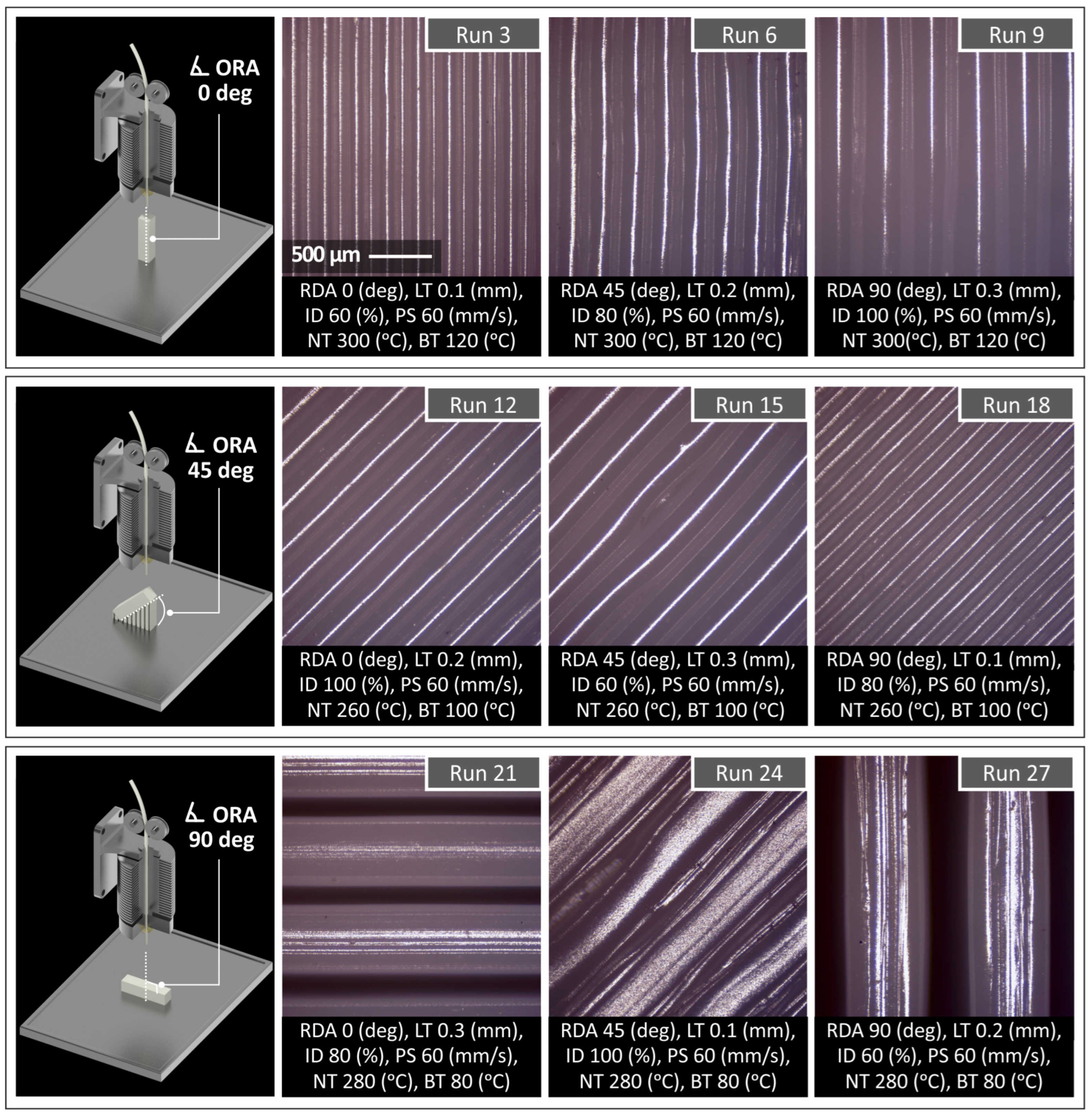
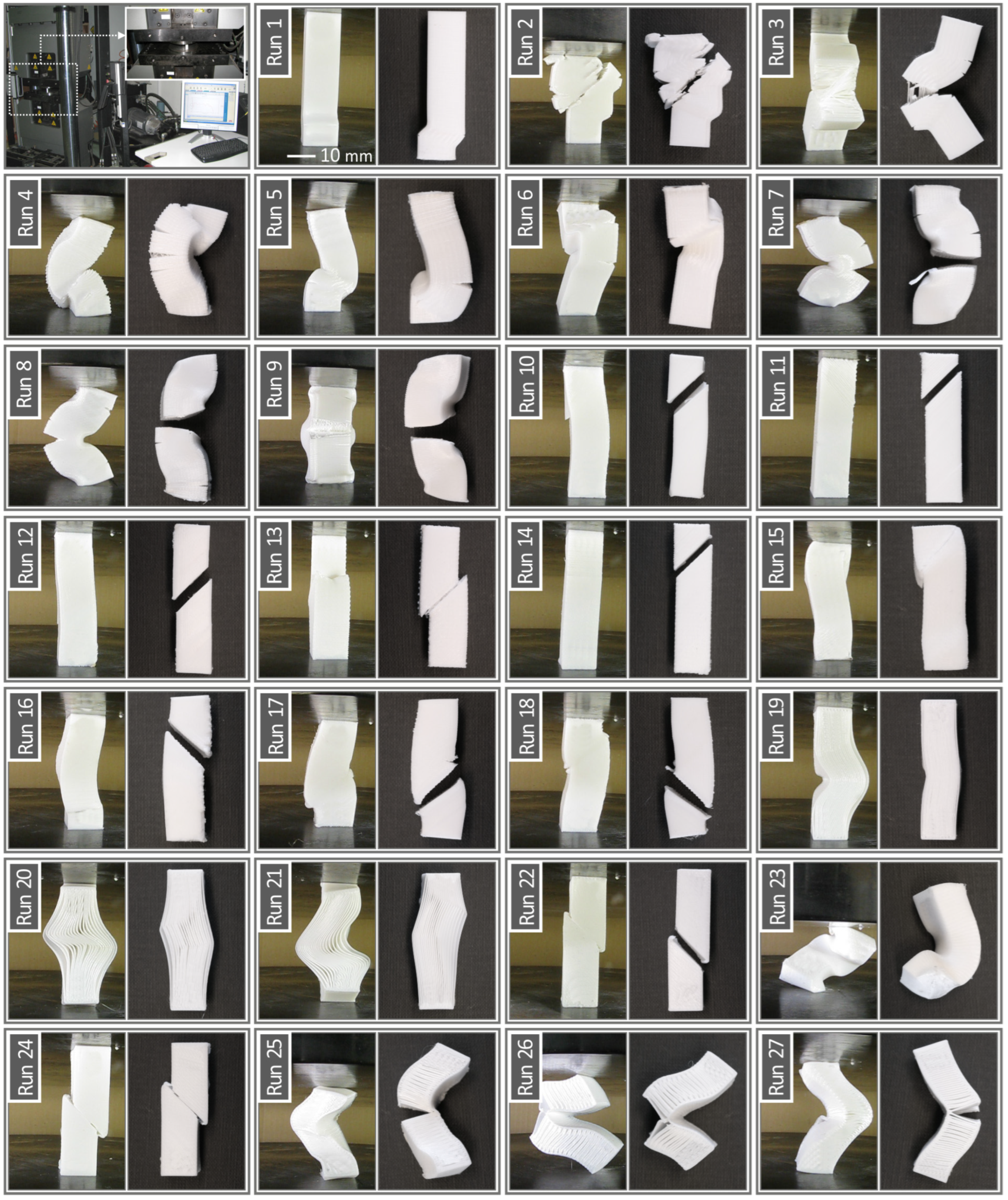
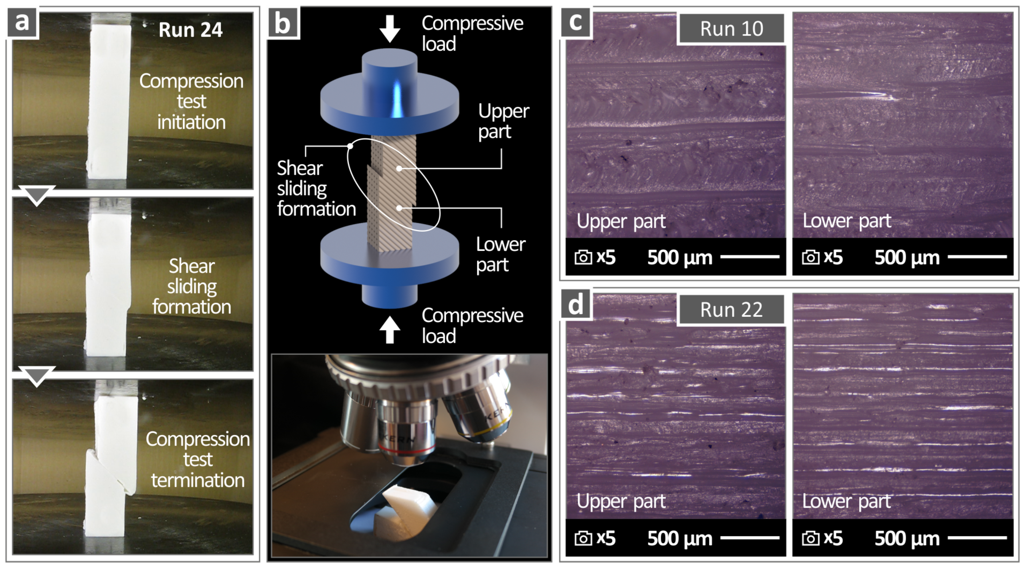
3.1. Examination of the Morphological Characteristics of the Samples and Their Behavior during the Compression Test

Figure 4 depicts top surface images acquired with optical microscopy from the samples. Images were taken on samples built with various control parameter values. Due to the various 3D printing parameters utilized in each sample, the changes in the 3D printing structure can be observed. An error-free 3D printing structure is shown in every image, demonstrating that the control parameter levels were suitable for producing the PC samples using MEX 3D printing. Please refer to this work’s Supplementary Material, where a microscope image from each of this work’s runs is displayed.

Compression tests are performed to ascertain the compressive strength of the 3D-printed specimens fabricated under various printing parameters, as well as to study and analyze the way they are prone to fail. Figure 5 illustrates the specimens subjected to a compression test according to the ASTM D695 standard. Based on the conducted compression tests, a classification of the resulting compressive failure modes can be established. The failure modes are grouped into three main failure types and can be further distinguished into subcategories. The first one pertains to kinking failure, either single or multiple (runs 1, 2, 3, 4, 5, 6). The kinking plane is formed at an angle of 45° to the specimen’s longitudinal axis, where the maximum shear stress occurs. The second failure type, characterized as buckling failure, consists of three discrete failure modes, i.e., lateral buckling (runs 7, 8, 9), buckling with interlaminar delamination (runs 19, 20, 21), and buckling accompanied by interfacial debonding (runs 25, 26, 27). Finally, the third failure type observed concerns shear failure comprising two distinct secondary modes, i.e., sliding shear (runs 10, 11, 12, 14) with a brittle fracture or successive degradation (runs 13, 15), and flexural shear failure (runs 16, 17, 18).

To explain the failure mechanism of the specimens, each type of failure mode is related to the 3D printing settings. It was noticed that the failure mode of the specimens is primarily dependent on the printing orientation angle (ORA). For a printing angle of 0^o, the specimens exhibit flexural failure either of kinking type or lateral buckling type, demonstrating maximum compressive strength in comparison to other printing angle values, which is even enhanced proportionally by the infill density (ID). Regarding a printing orientation angle of 45°, it is obvious that it leads to shear failure since sliding at the shear plane of 45° angle is triggered. Shearing is happening in the direction perpendicular to the filament strands deposited on the shear plane.

A printing angle of 90° leads to flexural failure either with interlaminar delamination in the case of the raster deposition angle (RDA) being equal to 0° or with interfacial debonding between adjacent filaments for RDA equal to 90°. The raster deposition angle (RDA) plays a supplemental role by modifying the principal failure mechanism. For example, the RDA angle of 45° generally alters the specimen’s failure, either by the shearing deformation with respect to the longitudinal axis or by preventing the separation of layers due to high interlaminar stresses acting on the interface between two adjacent layers [72,73,74,75,76]. Finally, the test results showed that the ultimate compressive resistance of the 3D-printed specimens is consistently related to the infill density (ID). The ultimate compressive resistance is defined as the maximum compressive load the specimen is capable of withstanding during the compression test. That means that by the ultimate compression load, a rupture occurs, indicating the initialization of the material failure. Regardless of the type of failure mode taking place, the infill density (ID) of the specimen enhances the compressive strength. With respect to the contribution of the other 3D printing settings, i.e., PS, BT, NT, on the failure mode of the specimens, the results prove that these parameters do not notably affect the compressive failure mode.

Figure 6 visualizes the methodology of investigating the 3D-printed PLA specimens’ failure caused by applying compressive load. The particular case presented here concerns the shear failure mode. The test specimen is placed between the plates of the compression tool, taking care to align its longitudinal axis with the center line of the plunger and to ensure that the ends of the specimen are parallel to the plates of the compression tool. Subsequently, the compression load is applied by axial movement of the plunger at the standard testing speed of 1.3 mm/min. While the specimen is exposed to a compressive load and gradually undergoes deformation, shear failure is initiated depending on the printed structure of the specimen. The compressive load is applied by the Instron KN1200 testing machine, which is suitable for these types of tests and was used in this work to conduct the compressive tests until the specimen completely fails. To explore the failure mechanism, the fractured surfaces are examined by microscopy. The micrograph images of two representative specimen failures (runs 10 and 22) reveal the sliding marks clearly formed on the PC strands being stressed under shear loading. The fracture plane where the shear failure occurs has an inclination of 45° to the loading axis due to the fact that on this plane, the maximum shear stresses are induced. In both cases presented here, mobilization of sliding fracture is facilitated from the specimens’ structure due to the intrinsic shear plane built in.

3.2. Design of Experiment, Experimental Results, and Statistical Analysis

The control parameter levels are shown in

Table 1. Taguchi L27 design: control parameters and levels.

Run	ORA	RDA	LT	ID	PS	NT	BT
1	0	0	0.1	60	20	260	80
2	0	0	0.1	60	40	280	100
3	0	0	0.1	60	60	300	120
4	0	45	0.2	80	20	260	80
5	0	45	0.2	80	40	280	100
6	0	45	0.2	80	60	300	120
7	0	90	0.3	100	20	260	80
8	0	90	0.3	100	40	280	100
9	0	90	0.3	100	60	300	120
10	45	0	0.2	100	20	280	120
11	45	0	0.2	100	40	300	80
12	45	0	0.2	100	60	260	100
13	45	45	0.3	60	20	280	120
14	45	45	0.3	60	40	300	80
15	45	45	0.3	60	60	260	100
16	45	90	0.1	80	20	280	120
17	45	90	0.1	80	40	300	80
18	45	90	0.1	80	60	260	100
19	90	0	0.3	80	20	300	100
20	90	0	0.3	80	40	260	120
21	90	0	0.3	80	60	280	80
22	90	45	0.1	100	20	300	100
23	90	45	0.1	100	40	260	120
24	90	45	0.1	100	60	280	80
25	90	90	0.2	60	20	300	100
26	90	90	0.2	60	40	260	120
27	90	90	0.2	60	60	280	80

, whereas

Table 2. Mean average values and standard deviations of measured responses for weight, printing time, compressive strength (sB), compressive modulus of elasticity (E), and compressive toughness.

Run	Weight (g)	Printing Time (s)	sB [MPa]	E [MPa]	Toughness [MJ/m3]
1	6.83 ± 0.21	7318.80 ± 1656.75	47.65 ± 3.96	1062.93 ± 71.46	4.27 ± 0.14
2	8.33 ± 0.21	4326.00 ± 973.56	50.72 ± 0.44	1132.37 ± 13.40	4.66 ± 0.13
3	6.70 ± 0.06	3340.20 ± 721.74	51.63 ± 1.00	1118.10 ± 26.88	5.22 ± 0.49
4	8.33 ± 0.18	3621.80 ± 722.55	58.88 ± 0.38	1191.34 ± 12.06	7.75 ± 0.16
5	8.46 ± 0.41	2557.00 ± 474.86	60.77 ± 0.61	1196.78 ± 17.21	7.93 ± 0.13
6	7.68 ± 0.36	1868.20 ± 367.67	62.84 ± 1.26	1155.62 ± 45.74	8.15 ± 0.37
7	9.52 ± 0.10	3431.20 ± 705.09	64.28 ± 2.57	1143.33 ± 38.62	9.15 ± 0.39
8	9.47 ± 0.04	1953.00 ± 369.39	62.77 ± 0.70	1166.96 ± 54.74	8.72 ± 0.13
9	9.42 ± 0.18	1475.00 ± 309.73	62.14 ± 0.97	1177.49 ± 13.82	8.45 ± 0.27
10	9.55 ± 0.23	6906.20 ± 1201.23	55.84 ± 2.71	886.82 ± 95.62	8.34 ± 0.43
11	9.45 ± 0.05	4348.00 ± 815.67	55.10 ± 1.66	825.61 ± 70.70	7.94 ± 1.63
12	8.81 ± 0.07	3422.00 ± 691.65	56.68 ± 0.98	887.99 ± 36.12	8.95 ± 0.14
13	5.80 ± 0.04	4458.00 ± 595.64	24.75 ± 0.59	410.29 ± 30.55	3.76 ± 0.09
14	6.61 ± 0.06	2399.00 ± 429.45	26.26 ± 0.44	437.88 ± 39.41	4.16 ± 0.10
15	6.57 ± 0.09	2095.20 ± 466.22	23.14 ± 1.89	475.80 ± 34.23	3.37 ± 0.62
16	8.15 ± 0.44	9484.00 ± 170.21	34.03 ± 4.25	523.85 ± 91.06	4.85 ± 0.89
17	8.30 ± 0.08	6921.00 ± 1519.48	29.35 ± 1.67	556.02 ± 81.62	4.22 ± 0.05
18	8.21 ± 0.17	5927.80 ± 1173.14	35.40 ± 0.34	693.81 ± 38.12	5.17 ± 0.23
19	7.41 ± 0.04	2745.60 ± 559.16	54.33 ± 4.88	1142.79 ± 23.90	3.65 ± 0.63
20	7.20 ± 0.13	1202.00 ± 238.05	38.68 ± 9.24	954.44 ± 122.89	3.54 ± 1.45
21	6.68 ± 0.10	1893.00 ± 331.64	34.44 ± 6.39	873.71 ± 111.67	2.92 ± 0.89
22	7.54 ± 0.30	7859.00 ± 1649.02	65.23 ± 3.56	1138.30 ± 99.48	9.38 ± 0.25
23	9.63 ± 0.43	8291.80 ± 1830.20	67.08 ± 3.00	1107.30 ± 53.79	9.06 ± 0.69
24	8.75 ± 0.40	3954.00 ± 802.05	52.23 ± 6.07	817.24 ± 157.84	7.00 ± 0.82
25	6.62 ± 0.16	2300.80 ± 432.62	16.59 ± 1.55	331.94 ± 20.63	2.29 ± 0.15
26	6.15 ± 0.09	1891.80 ± 387.23	20.57 ± 2.06	376.71 ± 15.25	2.53 ± 0.14
27	6.47 ± 0.10	996.00 ± 193.81	23.25 ± 1.34	435.20 ± 127.42	3.20 ± 0.22

and

Table 3. Mean average values and standard deviations of measured responses for EPC, SPE, SPP, area to nominal, and volume to nominal.

Run	EPC (MJ)	SPE (MJ/g)	SPP (kW/g)	Area 2 Nom [%]	Volume 2 Nom [%]
1	1.627 ± 0.309	0.238 ± 0.045	0.035 ± 0.012	71.32 ± 0.74	68.18 ± 0.68
2	1.822 ± 0.378	0.220 ± 0.049	0.052 ± 0.012	96.98 ± 0.47	96.45 ± 0.55
3	1.217 ± 0.337	0.182 ± 0.051	0.056 ± 0.019	101.09 ± 0.18	100.35 ± 0.29
4	1.008 ± 0.265	0.121 ± 0.033	0.035 ± 0.013	99.57 ± 0.23	99.48 ± 0.39
5	0.929 ± 0.246	0.110 ± 0.027	0.044 ± 0.013	102.18 ± 0.49	100.43 ± 0.64
6	0.828 ± 0.244	0.108 ± 0.033	0.062 ± 0.031	99.45 ± 0.29	97.80 ± 0.25
7	0.857 ± 0.247	0.090 ± 0.026	0.027 ± 0.010	103.24 ± 0.46	101.01 ± 0.64
8	0.835 ± 0.241	0.088 ± 0.026	0.047 ± 0.017	98.37 ± 0.75	96.71 ± 0.77
9	0.540 ± 0.167	0.057 ± 0.018	0.040 ± 0.013	104.14 ± 0.67	103.21 ± 0.62
10	1.692 ± 0.460	0.177 ± 0.047	0.027 ± 0.011	97.65 ± 0.44	97.34 ± 0.55
11	1.116 ± 0.223	0.118 ± 0.023	0.027 ± 0.005	99.64 ± 0.49	98.99 ± 0.53
12	1.584 ± 0.345	0.180 ± 0.039	0.053 ± 0.012	98.33 ± 0.36	98.20 ± 0.42
13	0.965 ± 0.179	0.166 ± 0.031	0.037 ± 0.002	96.78 ± 0.55	96.67 ± 0.58
14	0.547 ± 0.158	0.083 ± 0.024	0.036 ± 0.012	97.90 ± 1.22	98.21 ± 1.27
15	0.756 ± 0.182	0.115 ± 0.027	0.057 ± 0.019	100.54 ± 1.27	100.36 ± 1.27
16	4.003 ± 0.366	0.494 ± 0.070	0.052 ± 0.007	99.19 ± 1.23	98.59 ± 1.21
17	1.842 ± 0.580	0.222 ± 0.072	0.034 ± 0.014	98.21 ± 0.67	98.31 ± 0.68
18	1.728 ± 0.398	0.210 ± 0.048	0.038 ± 0.015	101.52 ± 0.90	101.16 ± 0.82
19	1.332 ± 0.395	0.180 ± 0.053	0.069 ± 0.029	99.42 ± 0.23	99.24 ± 0.32
20	0.612 ± 0.182	0.085 ± 0.025	0.074 ± 0.028	98.52 ± 0.62	97.94 ± 0.53
21	0.540 ± 0.163	0.081 ± 0.026	0.044 ± 0.018	91.13 ± 0.34	90.63 ± 0.35
22	4.997 ± 0.844	0.663 ± 0.112	0.086 ± 0.014	98.01 ± 0.51	97.49 ± 0.49
23	5.136 ± 0.312	0.535 ± 0.056	0.068 ± 0.019	103.09 ± 0.61	103.16 ± 0.59
24	3.353 ± 0.874	0.383 ± 0.098	0.101 ± 0.032	97.73 ± 0.62	97.48 ± 0.71
25	0.324 ± 0.099	0.049 ± 0.016	0.022 ± 0.009	97.54 ± 0.20	97.10 ± 0.18
26	0.828 ± 0.223	0.134 ± 0.035	0.075 ± 0.033	97.22 ± 0.72	96.84 ± 0.79
27	0.331 ± 0.064	0.051 ± 0.010	0.054 ± 0.018	100.79 ± 0.49	100.58 ± 0.48

present for each run carried out in this study, the average response parameters values and their deviation, as they were determined in the corresponding experiments by the authors of this work within the context of this specific study. More specifically, Table 2 depicts the weight (g), printing time (s), compressive strength (MPa), compressive modulus of elasticity (MPa), and compressive toughness (MJ/m³) response parameter results, and Table 3 depicts the results for EPC (MJ), SPE (MJ/g), SPP (kW/g), area to nominal (%), and volume to nominal (%). Please refer to this work’s Supplementary Material, where an optical microscope image from each of this work’s runs is displayed.

In Figure 7, by analyzing the experimental results of this work, considering the printing time (s), the weight (g), the compressive strength (MPa), and the EPC (MJ), box plots were produced:

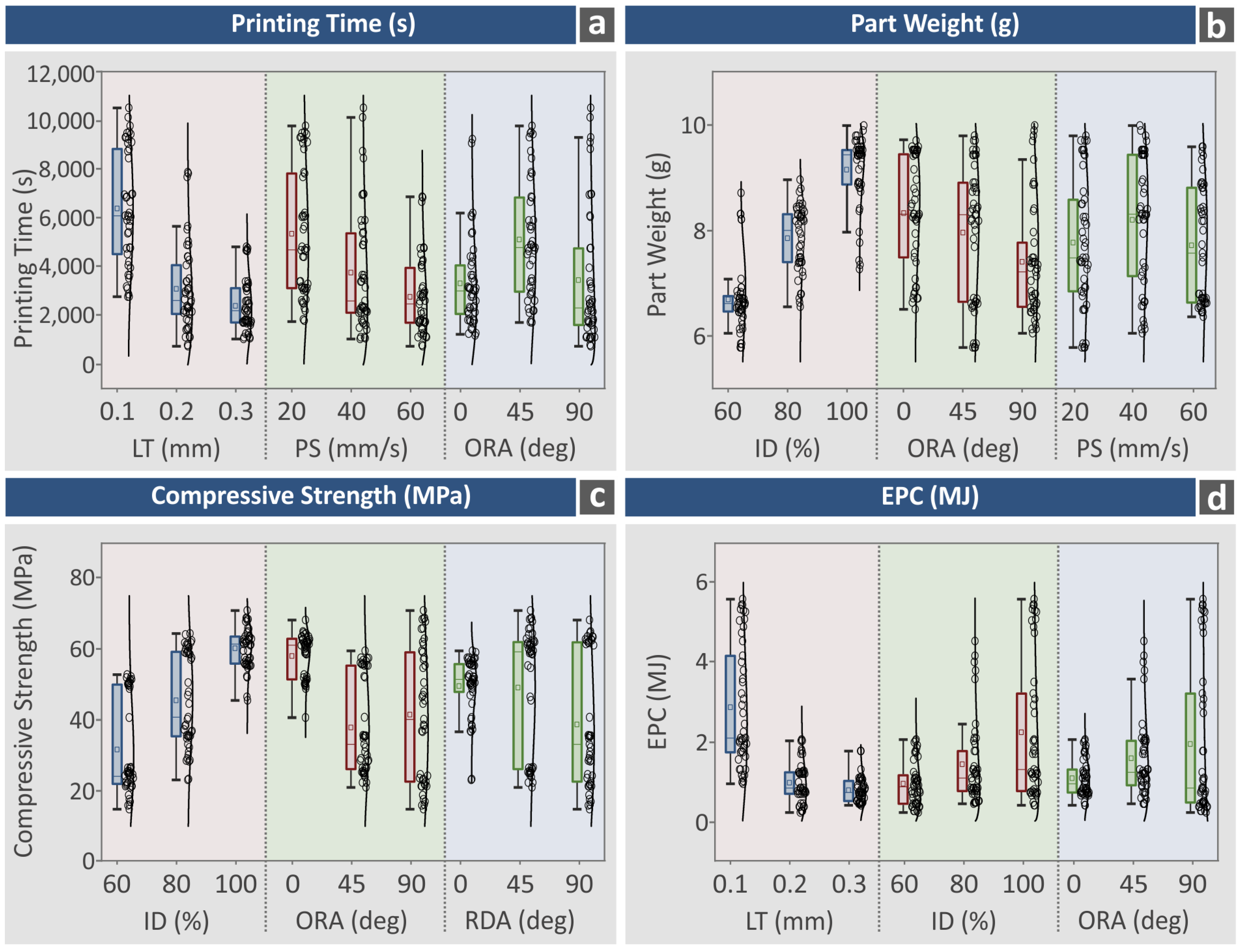
• For the printing time (s), only an LT of 0.3 mm shows a compact response. All the other parameters and levels show a scatter response, indicating a strong influence on the printing time (s) response parameter.
• For the part weight (g), an ID of 60% shows a compact response. All the other parameters and levels show a scatter response, indicating a strong influence on the part weight (g) response parameter.
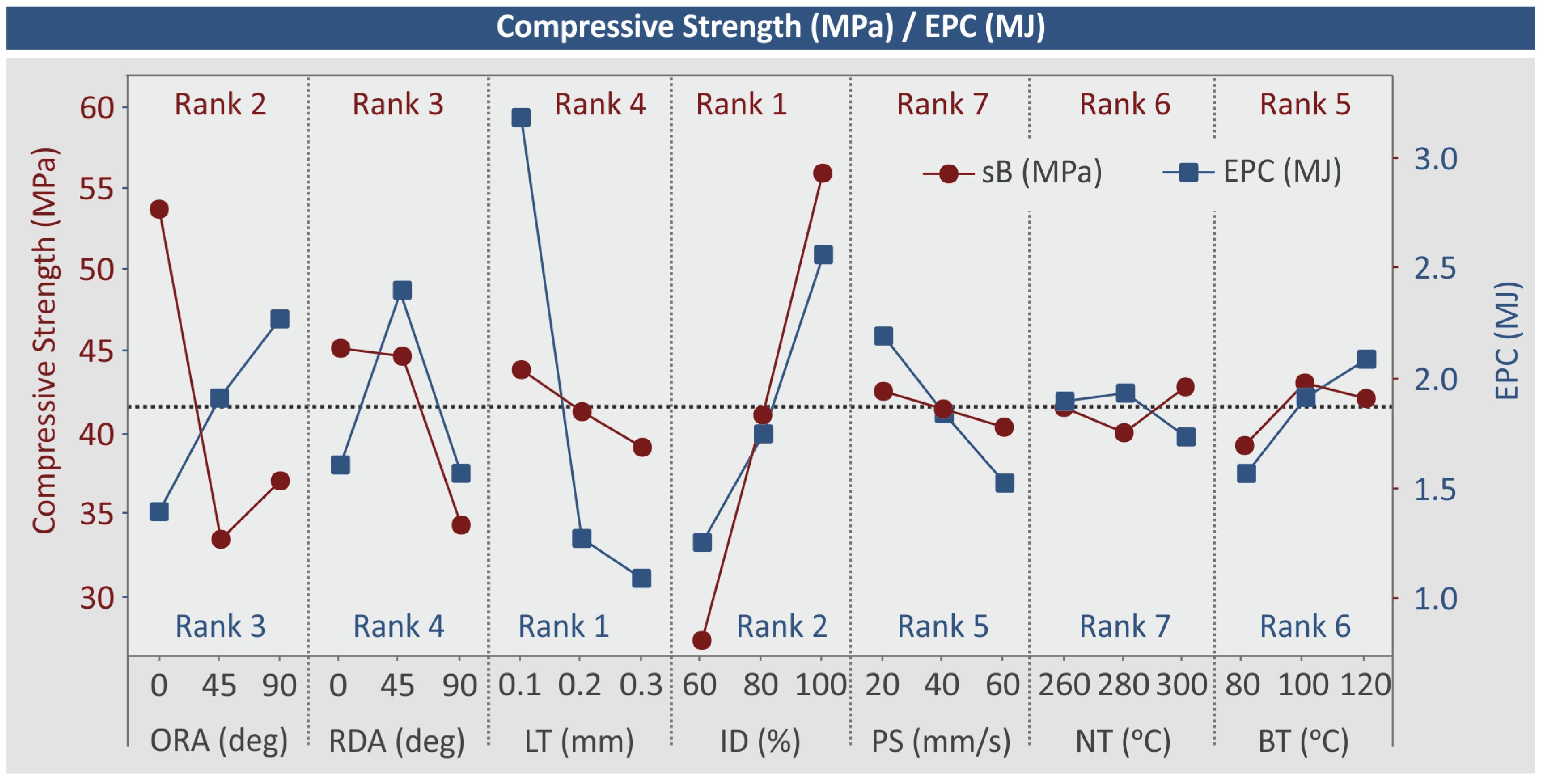
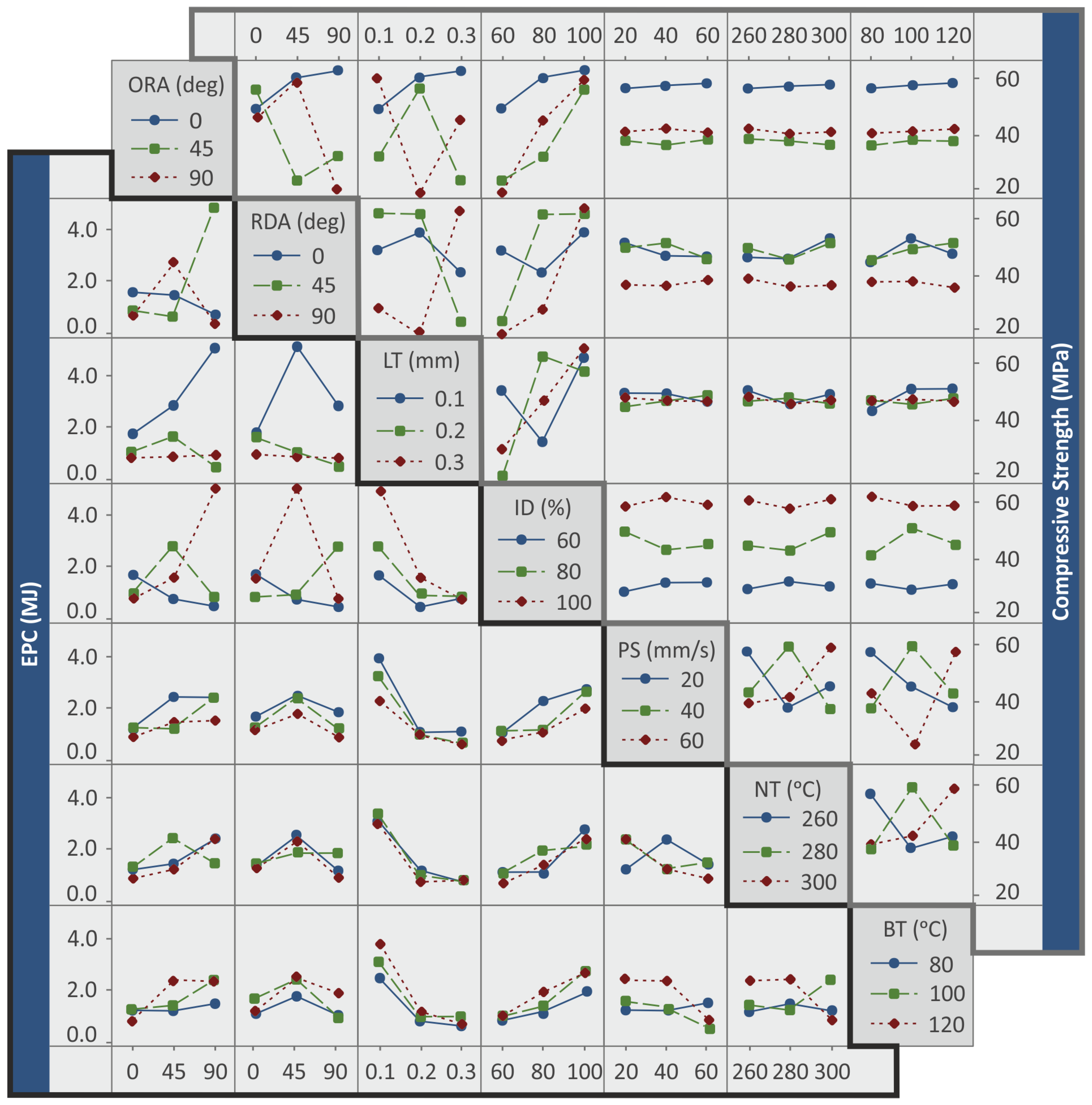
• For the compressive strength (MPa), an ID of 60% and 100%, ORA 0 deg, and RDA 0 deg show a compact response. All the other parameters and levels show a scatter response, indicating a strong influence on the compressive strength (MPa) response parameter.
• For the EPC (MJ), LT of 0.2 mm and 0.3 mm, ID of 60%, and ORA 0 deg show a compact response. All the other parameters and levels show a scatter response, indicating a strong influence on the EPC (MJ) response parameter.

MEP plots for the response are presented in Figure 8 and Figure 9, and the Supplementary Material of this work:

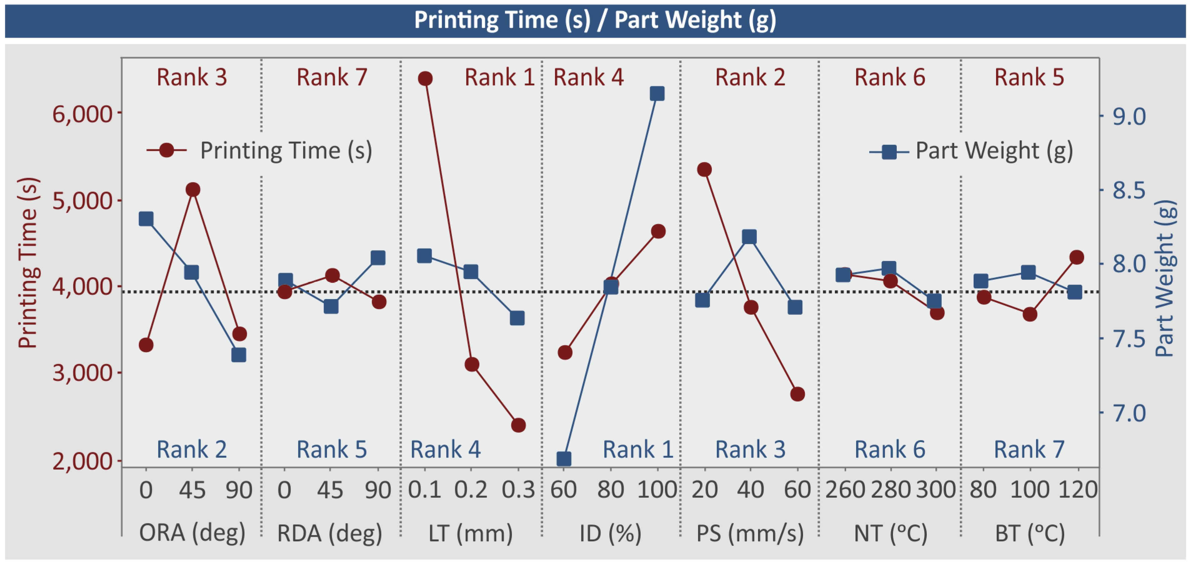
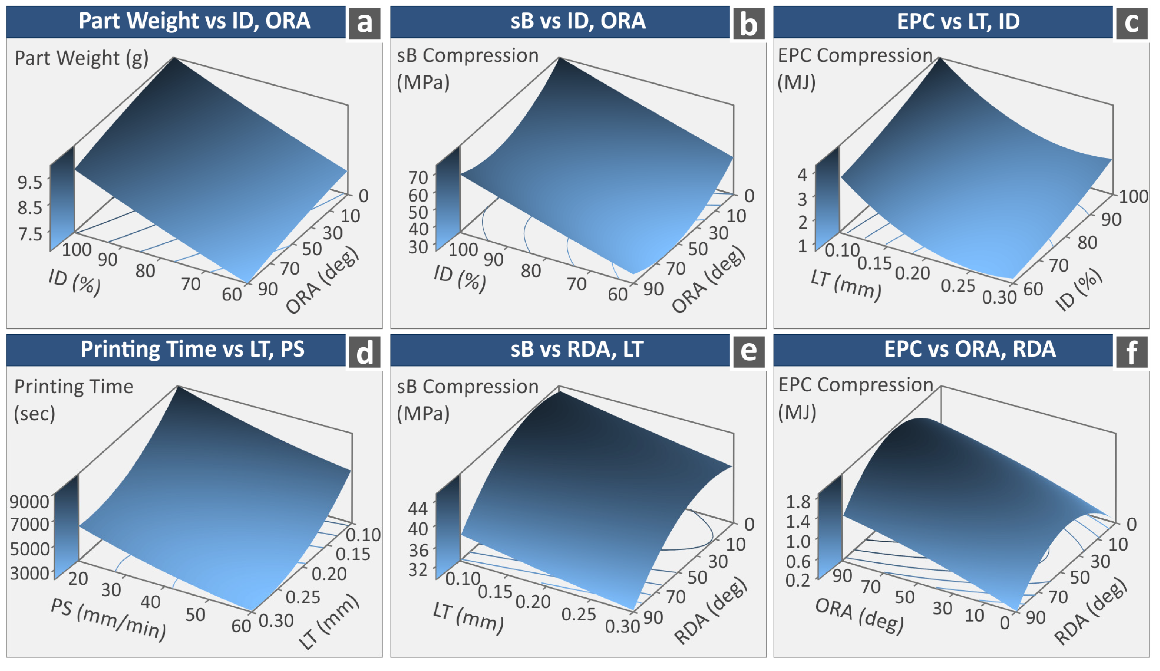
• For the printing time (s), LT (mm) is the most critical parameter (rank No. 1), and then PS (mm/s). The increase in both leads to a decrease in the printing time (s). The increase in ID increases the printing time (s). The median value of 45 deg for the ORA increases the printing time (s), while low and high values lead to reduced printing time (s) values. The remaining control parameters (BT, NT, and RDA) do not significantly affect the printing time (s) response parameter, with RDA being the least important control parameter.
• For the part weight (g), ID is the most important control parameter (rank No. 1). The increase in ID increases the part weight (g). The rank No. 2 control parameter is ORA, with the increase in the control parameter decreasing the part weight (g). The remaining control parameters (PS, LT, RDA, NT, and BT) do not significantly affect the part weight (g) response parameter, with BT being the least important control parameter.
• For the compressive strength (MPa), ID (%) is the most critical parameter (rank No. 1), and then ORA (deg). The increase in ID leads to an increase in compressive strength (MPa). Higher compressive strength (MPa) strength values are achieved with low ORA and RDA values. The increase in LT (mm) decreases compressive strength (MPa). The remaining control parameters (PS, NT, and BT) do not significantly affect the compressive strength (MPa) response parameter, with PS being the least important control parameter.
• For the EPC (MJ), LT (mm) is the most critical parameter (rank No. 1), and then ID (%). Higher LT (mm) values decrease the EPC (MJ) values, while low ID (%) values achieve the same effect. The increase in ORA (deg) increases the EPC (MJ). For the RDA (deg) control parameter, the median values resulted in higher EPC (MJ) values. Higher PS (mm/s) values decrease the EPC (MJ). Lower BT (°C) values also decrease the EPC (MJ). Only the NT (°C) control parameter had no significant effect on this metric, and it was at the same time the least important control parameter for the EPC (MJ) response parameter.

MEPs are not sufficient to depict the interaction between the control parameters, and thus, interaction plots were formed (Figure 10, additional interaction plots are available in the Supplementary Material of this work) to depict such connections. For the compressive strength (MPa) and the EPC (MJ), the interaction plot findings are depicted in

Table 4. Interaction plot findings.

Metrics	Compressive Strength (MPa)		EPC (MJ)
Control Parameters	Synergistic	Antagonistic	Synergistic	Antagonistic
ORA	PS, NT, and BT	RDA, LT, and ID	PS, NT, and BT	RDA, LT, and ID
RDA	PS, NT, and BT	LT, ID, and ORA	PS, NT, and BT	LT, ID, and ORA
LT	PS, NT, and BT	ID, RDA, and ORA	PS, NT, and BT	ID, RDA, and ORA
ID	PS, NT, and BT	LT, RDA, and ORA	PS, NT, LT, and BT	RDA and ORA
PS	ID, LT, RDA, and ORA	NT and BT	ID, LT, RDA, and ORA	NT and BT
NT	ID, LT, RDA, and ORA	PS and BT	ID, LT, RDA, and ORA	PS and BT

.

3.3. Regression Analysis

The reduced quadratic regression model (RQRM) for each response is calculated:

$${\mathrm{Y}}_{\mathrm{k}}={\mathrm{a}}_{\mathrm{k}}+{\displaystyle \sum }_{\mathrm{i}=1}^{\mathrm{n}}{\mathrm{b}}_{\mathrm{i},\mathrm{k}}{\mathrm{x}}_{\mathrm{i}}+{\displaystyle \sum }_{\mathrm{i}=1}^{\mathrm{n}}{\mathrm{c}}_{\mathrm{i},\mathrm{k}}{\mathrm{x}}_{\mathrm{i}}^2+{\mathrm{e}}_{\mathrm{k}}$$

(6)

where k represents the quality output (e.g., weight, printing time, compressive strength, compressive modulus of elasticity, compressive toughness, EPC, SPE), a is a constant value, b are the coefficients of the linear terms, c are the coefficients of the quadratic terms, e is the error, and x_i refers to the seven (n = 7) control parameters, i.e., the orientation angle, raster deposition angle, layer thickness, infill density, printing speed, nozzle temperature, and bed temperature.

The quadratic regression model (QRM) for each response is calculated:

$${\mathrm{Y}}_{\mathrm{k}}={\mathrm{a}}_{\mathrm{i},\mathrm{k}}+{\displaystyle \sum }_{\mathrm{i}=1}^{\mathrm{n}}{\mathrm{b}}_{\mathrm{i},\mathrm{k}}{\mathrm{x}}_{\mathrm{i}}+{\displaystyle \sum }_{\mathrm{i}=1}^{\mathrm{n}}{\mathrm{c}}_{\mathrm{i},\mathrm{k}}{\mathrm{x}}_{\mathrm{i}}^2+{\displaystyle \sum }_{\mathrm{i}}{\displaystyle \sum }_{\mathrm{j}}{\mathrm{d}}_{\mathrm{ij},\mathrm{k}}{\mathrm{x}}_{\mathrm{i}}{\mathrm{x}}_{\mathrm{j}}+{\mathrm{e}}_{\mathrm{k}}$$

(7)

where k represents the response output (e.g., SPP, area to nominal, volume to nominal), a is a constant value, b refers to the coefficients of the linear terms, c refers to the coefficients of the quadratic terms, d refers to the coefficients of the two-way interaction terms, e is the error, and x_i refers to the seven (n = 7) control parameters, i.e., the orientation angle, raster deposition angle, layer thickness, infill density, printing speed, nozzle temperature, and bed temperature.

The regression analysis for the metrics evaluated in this work is presented in corresponding tables provided in the Supplementary Material of this work (one for each metric). The corresponding predicting models formed for each metric are shown below (Equations (8)–(17)):

• Weight (g): the F-value is 60.09 (>4), and the P-value is almost zero. The regression values are higher than 84.20%, indicating that model (8) is sufficient for the prediction of this specific metric.
• Printing time (s): the F-value is 47.63 (>4), and the P-value is almost zero. The regression values are higher than 80.70%, indicating that the model (9) is sufficient for the prediction of this specific metric.
• Compression strength (MPa): the F-value is 110.32 (>4), and the P-value is almost zero. The regression values are higher than 90.88%, indicating that the model (10) is sufficient for the prediction of this specific metric.
• Compression modulus of elasticity (MPa): the F-value is 111.95 (>4), and the P-value is almost zero. The regression values are higher than 91.00%, indicating that the model (11) is sufficient for the prediction of this specific metric.
• Compression toughness (MJ/m³): the F-value is 103.93 (>4), and the P-value is almost zero. The regression values are higher than 90.36%, indicating that the model (12) is sufficient for the prediction of this specific metric.
• EPC (MJ): the F-value is 61.28 (>4), and the P-value is almost zero. The regression values are higher than 84.47%, indicating that the model (13) is sufficient for the prediction of this specific metric.
• SPE (MJ/g): the F-value is 48.28 (>4), and the P-value is almost zero. The regression values are higher than 80.92%, indicating that the model (14) is sufficient for the prediction of this specific metric.
• SPP (kW/g): the F-value is 5.03 (>4), and the P-value is almost zero. The regression values are higher than 24.56% (15). These results are marginal, and the prediction model accuracy is expected to be low for this specific metric.
• Area2Nom (%): the F-value is 20.67 (>4), and the P-value is almost zero. The regression values are higher than 69.76% (16). These results are lower compared to the other metrics (except SPP). Although they are highly acceptable, these results indicate lower reliability in the prediction of the specific metric.
• Vol2Nom (%): the F-value is 18.00 (>4), and the P-value is almost zero. The regression values are higher than 66.52% (17). These results are lower compared to the other metrics (except SPP). Although they are highly acceptable, these results indicate lower reliability in the prediction of the specific metric.

$$\begin{array}{ll}\mathrm{Weight}=& -23.2-0.00605\times \mathrm{ORA}-0.00951\times \mathrm{RDA}+2.15\times \mathrm{LT}+0.0312\times \mathrm{ID}\\ & +0.0894\times \mathrm{PS}+0.179\times \mathrm{NT}+0.0428\times \mathrm{BT}-0.000046\times {\mathrm{ORA}}^2\\ & +0.000124\times {\mathrm{RDA}}^2-10.60\times {\mathrm{LT}}^2+0.000188\times {\mathrm{ID}}^2\\ & -0.001133\times {\mathrm{PS}}^2-0.000327\times {\mathrm{NT}}^2-0.000223\times {\mathrm{BT}}^2\end{array}$$

(8)

$$\begin{array}{ll}\mathrm{PrintingTime}=& -5241+77.82\times \mathrm{ORA}+9.30\times \mathrm{RDA}-71541\times \mathrm{LT}+72.0\times \mathrm{ID}\\ & -123.4\times \mathrm{PS}+191\times \mathrm{NT}-195.1\times \mathrm{BT}-0.8477\times {\mathrm{ORA}}^2\\ & -0.1187\times {\mathrm{RDA}}^2+\mathrm{129,172}\times {\mathrm{LT}}^2-0.233\times {\mathrm{ID}}^2+0.739\times {\mathrm{PS}}^2\\ & -0.360\times {\mathrm{NT}}^2+1.032\times {\mathrm{BT}}^2\end{array}$$

(9)

$$\begin{array}{ll}\mathrm{sB}=& 362-0.7102\times \mathrm{ORA}+0.1001\times \mathrm{RDA}-30.4\times \mathrm{LT}+0.525\times \mathrm{ID}-0.063\times \mathrm{PS}\\ & -2.94\times \mathrm{NT}+1.246\times \mathrm{BT}+0.005843\times {\mathrm{ORA}}^2\\ & -0.002439\times {\mathrm{RDA}}^2+17.0\times {\mathrm{LT}}^2+0.00118\times {\mathrm{ID}}^2\\ & +0.00010\times {\mathrm{PS}}^2+0.00531\times {\mathrm{NT}}^2-0.00587\times {\mathrm{BT}}^2\end{array}$$

(10)

$$\begin{array}{ll}\mathrm{E}=& 7277-19.037\times \mathrm{ORA}-1.651\times \mathrm{RDA}-3219\times \mathrm{LT}+45.90\times \mathrm{ID}-0.08\times \mathrm{PS}\\ & -69.3\times \mathrm{NT}+36.56\times \mathrm{BT}+0.16808\times {\mathrm{ORA}}^2-0.01567\times {\mathrm{RDA}}^2\\ & +7537\times {\mathrm{LT}}^2-0.2284\times {\mathrm{ID}}^2-0.0058\times {\mathrm{PS}}^2+0.1237\times {\mathrm{NT}}^2\\ & -0.1777\times {\mathrm{BT}}^2\end{array}$$

(11)

$$\begin{array}{ll}\mathrm{Toughness}=& 50.5-0.04132\times \mathrm{ORA}+0.05584\times \mathrm{RDA}+24.67\times \mathrm{LT}-0.1919\times \mathrm{ID}\\ & -0.0065\times \mathrm{PS}-0.349\times \mathrm{NT}+0.1129\times \mathrm{BT}+0.000175\times {\mathrm{ORA}}^2\\ & -0.000633\times {\mathrm{RDA}}^2-70.2\times {\mathrm{LT}}^2+0.001955\times {\mathrm{ID}}^2\\ & +0.000047\times {\mathrm{PS}}^2+0.000622\times {\mathrm{NT}}^2-0.000519\times {\mathrm{BT}}^2\end{array}$$

(12)

$$\begin{array}{ll}\mathrm{EPC}=& -18.3+0.01296\times \mathrm{ORA}+0.03477\times \mathrm{RDA}-44.70\times \mathrm{LT}-0.0316\times \mathrm{ID}\\ & -0.0203\times \mathrm{PS}+0.156\times \mathrm{NT}+0.0564\times \mathrm{BT}-0.000037\times {\mathrm{ORA}}^2\\ & -0.000390\times {\mathrm{RDA}}^2+85.72\times {\mathrm{LT}}^2+0.000400\times {\mathrm{ID}}^2\\ & +0.000048\times {\mathrm{PS}}^2-0.000286\times {\mathrm{NT}}^2-0.000218\times {\mathrm{BT}}^2\end{array}$$

(13)

$$\begin{array}{ll}\mathrm{SPE}=& -1.45+0.001552\times \mathrm{ORA}+0.004148\times \mathrm{RDA}-5.659\times \mathrm{LT}-0.00392\times \mathrm{ID}\\ & -0.00621\times \mathrm{PS}+0.0130\times \mathrm{NT}+0.00990\times \mathrm{BT}\\ & -0.000004\times {\mathrm{ORA}}^2-0.000047\times {\mathrm{RDA}}^2+11.09\times {\mathrm{LT}}^2\\ & +0.000043\times {\mathrm{ID}}^2+0.000049\times {\mathrm{PS}}^2-0.000023\times {\mathrm{NT}}^2\\ & -0.000042\times {\mathrm{BT}}^2\end{array}$$

(14)

$$\begin{array}{ll}\mathrm{SPP}=& -0.564-0.000419\times \mathrm{ORA}-0.00063\times \mathrm{RDA}+1.342\times \mathrm{LT}+0.00022\times \mathrm{ID}\\ & +0.000721\times \mathrm{PS}+0.00284\times \mathrm{NT}+0.00131\times \mathrm{BT}\\ & +0.000007\times {\mathrm{ORA}}^2-0.000006\times {\mathrm{RDA}}^2+0.835\times {\mathrm{LT}}^2\\ & -0.000000\times {\mathrm{ID}}^2-0.000002\times {\mathrm{PS}}^2-0.000003\times {\mathrm{NT}}^2\\ & -0.000007\times {\mathrm{BT}}^2+0.000007\times \mathrm{RDA}\times \mathrm{PS}\\ & -0.000000\times \mathrm{RDA}\times \mathrm{NT}+0.000010\times \mathrm{RDA}\times \mathrm{BT}\\ & -0.00267\times \mathrm{LT}\times \mathrm{PS}-0.00578\times \mathrm{LT}\times \mathrm{NT}\end{array}$$

(15)

$$\begin{array}{ll}\mathrm{Area}2\mathrm{Nom}=& 0.26+0.000576\times \mathrm{ORA}+0.01594\times \mathrm{RDA}-0.616\times \mathrm{LT}\\ & +0.00512\times \mathrm{ID}+0.00429\times \mathrm{PS}-0.00432\times \mathrm{NT}+0.01101\times \mathrm{BT}\\ & -0.000005\times {\mathrm{ORA}}^2-0.000010\times {\mathrm{RDA}}^2-1.531\times {\mathrm{LT}}^2\\ & -0.000025\times {\mathrm{ID}}^2-0.000037\times {\mathrm{PS}}^2+0.000010\times {\mathrm{NT}}^2\\ & -0.000040\times {\mathrm{BT}}^2-0.000020\times \mathrm{RDA}\times \mathrm{PS}\\ & -0.000034\times \mathrm{RDA}\times \mathrm{NT}-0.000042\times \mathrm{RDA}\times \mathrm{BT}\\ & +0.00226\times \mathrm{LT}\times \mathrm{PS}+0.00452\times \mathrm{LT}\times \mathrm{NT}\end{array}$$

(16)

$$\begin{array}{ll}\mathrm{Volume}2\mathrm{Nom}=& 0.25+0.000988\times \mathrm{ORA}+0.01664\times \mathrm{RDA}-0.90\times \mathrm{LT}\\ & +0.00527\times \mathrm{ID}+0.00470\times \mathrm{PS}-0.00452\times \mathrm{NT}+0.01131\times \mathrm{BT}\\ & -0.000009\times {\mathrm{ORA}}^2-0.000011\times {\mathrm{RDA}}^2-1.578\times {\mathrm{LT}}^2\\ & -0.000026\times {\mathrm{ID}}^2-0.000041\times {\mathrm{PS}}^2+0.000010\times {\mathrm{NT}}^2\\ & -0.000041\times {\mathrm{BT}}^2-0.000021\times \mathrm{RDA}\times \mathrm{PS}\\ & -0.000035\times \mathrm{RDA}\times \mathrm{NT}-0.000045\times \mathrm{RDA}\times \mathrm{BT}\\ & +0.00231\times \mathrm{LT}\times \mathrm{PS}+0.00559\times \mathrm{LT}\times \mathrm{NT}\end{array}$$

(17)

To identify the statistically important parameters for the metrics of this work, Pareto charts were formed, and they are presented in Figure 11 and Figure 12 below. Additional Pareto charts are available in the Supplementary Material of this work. In the Pareto charts, the parameters that cross the 1.98 margin are the statistically important parameters for each metric. On the right side of each Pareto chart, a graph shows a comparison between the experimental and the predicted values for each specific metric. In each such graph, the mean absolute percentage error (MAPE) [77] and the Durbin–Watson factor, which is a measurement indicator of the autocorrelation in the residuals, are presented. In Figure 11 and Figure 12 below, the following can be observed:

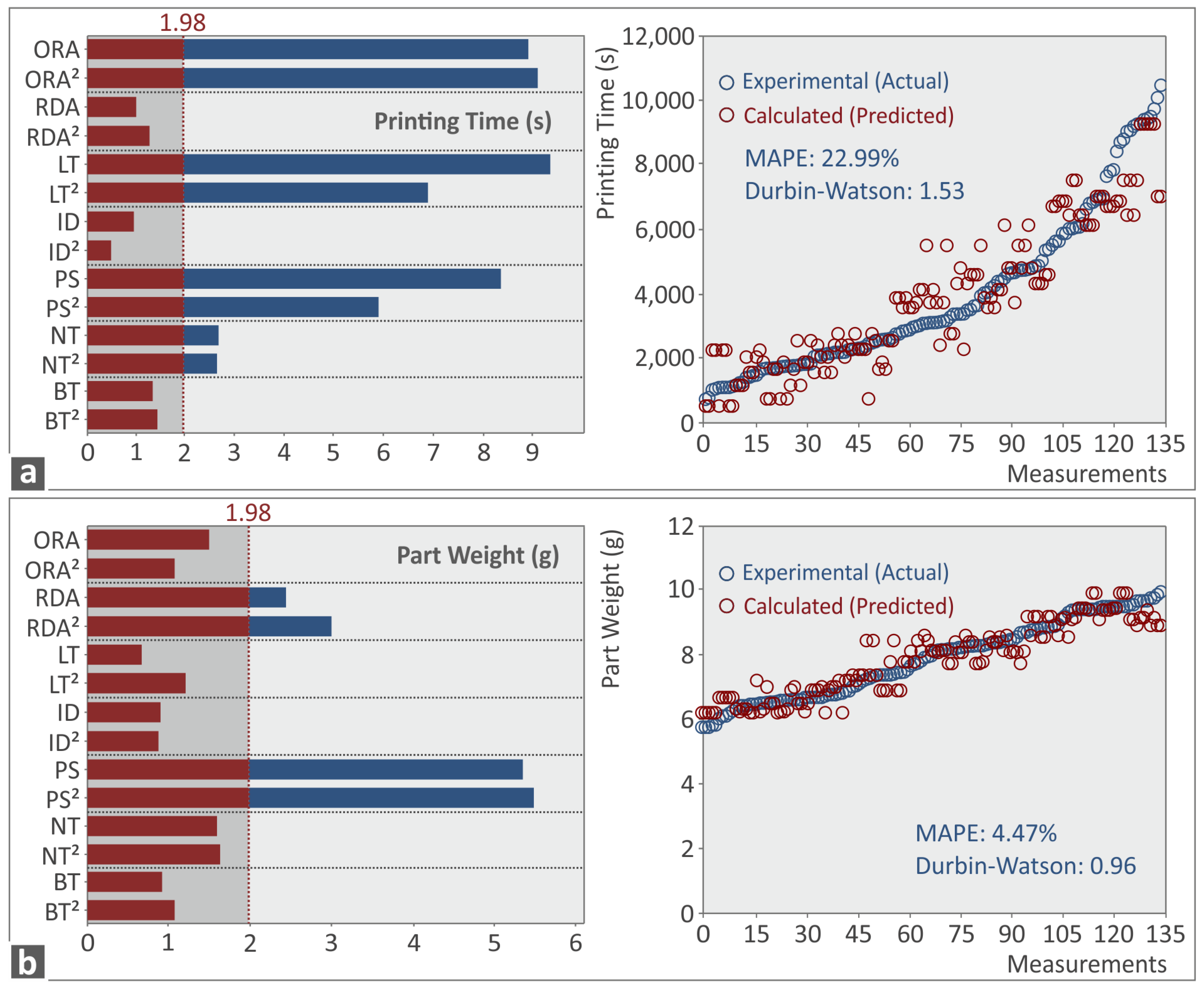
• Figure 11a (printing time—s): the statistically important parameters are ORA, ORA², LT, LT², PS, PS², NT, and NT². The MAPE is 22.99%, which is an acceptable result. The Durbin–Watson factor is 1.53, showing a positive autocorrelation of the prediction residuals.
• Figure 11b (part weight—g): the statistically important parameters are RDA, RDA², PS, and PS². The MAPE is 4.47%, which is a very acceptable result, verifying the reliability of the model. The Durbin–Watson factor is 0.96, showing a positive autocorrelation of the prediction residuals.
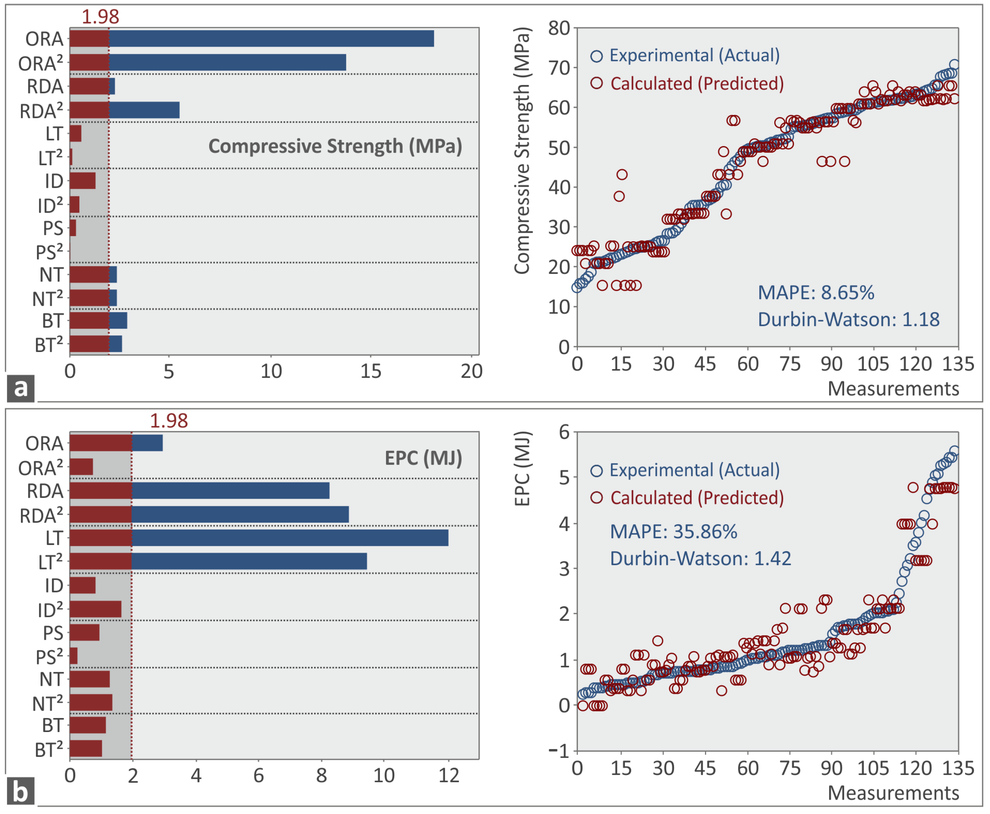
• Figure 12a (compressive strength—MPa): the statistically important parameters are ORA, ORA², RDA², NT, NT², BT, and BT². The MAPE is 8.65%, which is a very acceptable result, verifying the reliability of the model. The Durbin–Watson factor is 1.18, showing a positive autocorrelation of the prediction residuals.
• Figure 12b (EPC-MJ): statistically important parameters are ORA, RDA, RDA², LT, and LT². The MAPE is 35.86%, which is an acceptable result. The Durbin–Watson factor is 1.42, showing a positive autocorrelation of the prediction residuals.

Figure 13 shows, for some critical metrics of this work, three-dimensional surface graphs of the control parameters (rank No. 1 and 2) vs. the corresponding metric.

3.4. Confirmation Experiments

To verify the regression analysis and the prediction models forms, two confirmation runs were conducted, with five replicas each (runs 28 and 29).

Table 5. Control parameters for the confirmation runs.

Run	ORA	RDA	LT	ID	PS	NT	BT
28	0	20.9	0.1	100	20	300	106.3
29	0	90	0.26	60	60	300	80

presents the levels for the control parameters in each run. The experimental results for the metrics of this work in each run (average value and deviation) are presented in

Table 6. Mean average values and standard deviations of measured responses for weight, printing time, compressive strength, compressive modulus of elasticity, and compressive toughness for the confirmation runs.

Run	Weight (g)	Printing Time (s)	sB [MPa]	E [MPa]	Toughness [MJ/m3]
28	9.52 ± 0.11	10,854.60 ± 497.50	80.72 ± 2.04	1369.03 ± 46.07	10.23 ± 0.60
29	7.27 ± 0.24	1158.00 ± 144.19	42.46 ± 1.06	1068.52 ± 41.69	4.73 ± 0.10

and

Table 7. Mean average values and standard deviations of measured responses for EPC, SPE, SPP, area to nominal, and volume to nominal for the confirmation runs.

Run	EPC (MJ)	SPE (MJ/g)	SPP (kW/g)	Area 2 Nom [%]	Volume 2 Nom [%]
28	4.032 ± 0.405	0.423 ± 0.038	0.039 ± 0.002	91.55 ± 0.56	91.09 ± 0.70
29	0.518 ± 0.075	0.071 ± 0.010	0.062 ± 0.010	106.99 ± 0.51	87.90 ± 0.49

(the confirmation runs results are analytically accessible in the Supplementary Material of this work). The accuracy of the prediction models in the conformation runs is depicted in

Table 8. Validation table.

Run		28	29
Actual	sB (MPa)	80.72	42.46
	EPC (MJ)	4.03	0.52
Predicted	sB (MPa)	85.26	34.80
	EPC (MJ)	3.69	Vague
Absolute Error	sB (%)	5.62	18.03
	EPC (%)	8.52	Vague

, in which the actual and the predicted values for the metrics of this work are presented along with the deviation (error) between them. An eminent accuracy of the prediction models was found for run 28, with 5.62% and 8.52% deviation between the actual and the calculated compression strength (MPa) and EPC (MJ) values, respectively. For run 29, the accuracy of compression strength (MPa) was not as high as in run 28 (18.03%), while for the EPC (MJ) metric, the model failed to predict the expected value. This indicates that the control parameter levels were outside the limits for the specific metric. The acceptable limits of the prediction models were not within the scope of the current work. It should be noted that the compression strength and the EPC are the two main metrics related to the aims of this work. Therefore, they were the metrics that were more critical to be evaluated in the confirmation tests. Confirmation tests were conducted with the more suitable control parameter levels for each metric. Since the optimum parameter levels for each metric studied in this work differ, the extent of this work would be significantly increased if more metrics were considered in the confirmation tests.

4. Conclusions

In this study, the energy consumption, compressive strength, and two quality metrics of parts made with the high-performance PC polymer with MEX 3D printing were investigated compared to seven continuous, machine-independent, generic 3D printing settings. The study of energy consumption is directly related to the sustainability of the MEX 3D printing process, which is already a critical aspect of AM. Additionally, a thorough investigation was conducted on the performance of MEX 3D-printed parts when subjected to compressive load. The two quality parameters studied are related to the dimensional accuracy of the MEX 3D-printed parts, and it was shown how it is affected by seven different 3D printing settings when varying their values within limits determined by the literature review conducted in this work.

DOE and regression analysis ranked the importance of each 3D printing setting on the energy, mechanical properties under compression loading, and dimensional accuracy metrics studied in this work. Additionally, prediction models were compiled for each one of the ten metrics considered in this work. The accuracy of the prediction models was sufficient for direct industrial use in all metrics except the SPP, which showed reduced accuracy. A reduced accuracy of about 60% was also found for the two quality metrics in this work, i.e., actual to nominal for the samples’ cross-section area and volume. The validity of these prediction models was verified with two confirmation runs. In the confirmation runs, the predicted values for the compression strength were very accurate in both runs. In the second confirmation run, the model failed to predict the EPC value, showing that the prediction models function properly within limits for the control parameter levels.

No set of 3D printing settings optimizes both the energy and the mechanical properties metrics, indicating that priorities should be made for the optimization of the desirable metrics, with the models that can predict the expected values for the remaining metrics. Infill density was the most important parameter affecting the compression strength of the PC MEX 3D-printed parts. It was ranked No. 1 in importance, and high ID values (i.e., 100%) are recommended to achieve increased compression strength values. Low ORA values (i.e., 0 deg) also contribute to this result. Printing speed was the least important parameter for the compression strength metric. The layer thickness was the most important parameter (ranked as No. 1) affecting the energy consumption of the PC MEX 3D-printed parts. High values of LT (i.e., 0.3 mm) significantly reduce the energy consumption when 3D printing PC parts with the MEX process. Infill density also significantly affects energy consumption, and low values (i.e., 60%) are recommended when the energy requirements need to be minimum. Nozzle temperature was the least important parameter for this metric. To broaden the range of applicability for the current study’s findings, future work may expand on it by examining control parameter values in a new value range.

References

1. Freitas, D.; Almeida, H.A.; Bártolo, H.; Bártolo, P.J. Sustainability in extrusion-based additive manufacturing technologies. Prog. Addit. Manuf. 2016, 1, 65–78. [Google Scholar] [CrossRef]
2. Liu, Z.; Jiang, Q.; Zhang, Y.; Li, T.; Zhang, H.C. Sustainability of 3D printing: A critical review and recommendations. In Proceedings of the ASME 2016 11th International Manufacturing Science and Engineering Conference, Blacksburg, VI, USA, 27 June–1 July 2016; Volume 2, pp. 1–8. [Google Scholar] [CrossRef]
3. Malik, A.; Ul Haq, M.I.; Raina, A.; Gupta, K. 3D printing towards implementing Industry 4.0: Sustainability aspects, barriers and challenges. Ind. Rob. 2022, 49, 491–511. [Google Scholar] [CrossRef]
4. Jiang, J.; Fu, Y.F. A short survey of sustainable material extrusion additive manufacturing. Aust. J. Mech. Eng. 2020, 1–10. [Google Scholar] [CrossRef]
5. Dey, A.; Eagle, I.N.R.; Yodo, N. A review on filament materials for fused filament fabrication. J. Manuf. Mater. Process. 2021, 5, 69. [Google Scholar] [CrossRef]
6. Suárez, L.; Domínguez, M. Sustainability and environmental impact of fused deposition modelling (FDM) technologies. Int. J. Adv. Manuf. Technol. 2020, 106, 1267–1279. [Google Scholar] [CrossRef]
7. Khosravani, M.R.; Reinicke, T. On the environmental impacts of 3D printing technology. Appl. Mater. Today 2020, 20, 100689. [Google Scholar] [CrossRef]
8. Stoof, D.; Pickering, K. Sustainable composite fused deposition modelling filament using recycled pre-consumer polypropylene. Compos. Part B Eng. 2018, 135, 110–118. [Google Scholar] [CrossRef]
9. Fico, D.; Rizzo, D.; Casciaro, R.; Corcione, C.E. A Review of Polymer-Based Materials for Fused Filament Recycled Materials. Polymers 2022, 14, 465. [Google Scholar] [CrossRef]
10. Kumar, S.; Kazancoglu, Y.; Deniz, M.; Top, N.; Sahin, I. Optimizing fused deposition modelling parameters based on the design for additive manufacturing to enhance product sustainability. Comput. Ind. 2023, 145, 103833. [Google Scholar] [CrossRef]
11. Ramesh, P.; Vinodh, S. Analysis of factors influencing energy consumption of material extrusion-based additive manufacturing using interpretive structural modelling. Rapid Prototyp. J. 2021, 27, 1363–1377. [Google Scholar] [CrossRef]
12. Abeykoon, C.; McMillan, A.; Nguyen, B.K. Energy efficiency in extrusion-related polymer processing: A review of state of the art and potential efficiency improvements. Renew. Sustain. Energy Rev. 2021, 147, 111219. [Google Scholar] [CrossRef]
13. Kim, K.; Noh, H.; Park, K.; Jeon, H.W.; Lim, S. Characterization of power demand and energy consumption for fused filament fabrication using CFR-PEEK. Rapid Prototyp. J. 2022, 28, 1394–1406. [Google Scholar] [CrossRef]
14. Hassan, M.R.; Jeon, H.W.; Kim, G.; Park, K. The effects of infill patterns and infill percentages on energy consumption in fused filament fabrication using CFR-PEEK. Rapid Prototyp. J. 2021, 27, 1886–1899. [Google Scholar] [CrossRef]
15. De Bernardez, L.; Campana, G.; Mele, M.; Sanguineti, J.; Sandre, C.; Mur, S.M. Effects of infill patterns on part performances and energy consumption in acrylonitrile butadiene styrene fused filament fabrication via industrial-grade machine. Prog. Addit. Manuf. 2022, 1–13. [Google Scholar] [CrossRef]
16. El youbi El idrissi, M.A.; Laaouina, L.; Jeghal, A.; Tairi, H.; Zaki, M. Energy Consumption Prediction for Fused Deposition Modelling 3D Printing Using Machine Learning. Appl. Syst. Innov. 2022, 5, 86. [Google Scholar] [CrossRef]
17. Vidakis, N.; Kechagias, J.D.; Petousis, M.; Vakouftsi, F.; Mountakis, N. The effects of FFF 3D printing parameters on energy consumption. Mater. Manuf. Process. 2022, 1–18. [Google Scholar] [CrossRef]
18. Peng, T. Energy Modelling for FDM 3D Printing from a Life Cycle Perspective. Int. J. Manuf. Res. 2017, 11, 1. [Google Scholar] [CrossRef]
19. Hassan, M.R.; Noh, H.; Park, K.; Jeon, H.W. Simulating energy consumption based on material addition rates for material extrusion of CFR-PEEK: A trade-off between energy costs and cycle time. Int. J. Adv. Manuf. Technol. 2022, 120, 4597–4616. [Google Scholar] [CrossRef]
20. Tian, W.; Ma, J.; Alizadeh, M. Energy consumption optimization with geometric accuracy consideration for fused filament fabrication processes. Int. J. Adv. Manuf. Technol. 2019, 103, 3223–3233. [Google Scholar] [CrossRef]
21. Kausar, A. A review of filled and pristine polycarbonate blends and their applications. J. Plast. Film Sheeting 2018, 34, 60–97. [Google Scholar] [CrossRef]
22. Park, S.J.; Lee, J.E.; Lee, H.B.; Park, J.; Lee, N.K.; Son, Y.; Park, S.H. 3D printing of bio-based polycarbonate and its potential applications in ecofriendly indoor manufacturing. Addit. Manuf. 2020, 31, 100974. [Google Scholar] [CrossRef]
23. Reich, M.J.; Woern, A.L.; Tanikella, N.G.; Pearce, J.M. Mechanical properties and applications of recycled polycarbonate particle material extrusion-based additive manufacturing. Materials 2019, 12, 1642. [Google Scholar] [CrossRef] [PubMed]
24. Mallakpour, S.; Hussain, C.M. Handbook of Consumer Nanoproducts. Handb. Consum. Nanoproducts 2022, 257–281. [Google Scholar] [CrossRef]
25. Pedrosa, P.; Alves, E.; Barradas, N.P.; Fiedler, P.; Haueisen, J.; Vaz, F.; Fonseca, C. TiNx coated polycarbonate for bio-electrode applications. Corros. Sci. 2012, 56, 49–57. [Google Scholar] [CrossRef]
26. Pande, S.; Chaudhary, A.; Patel, D.; Singh, B.P.; Mathur, R.B. Mechanical and electrical properties of multiwall carbon nanotube/polycarbonate composites for electrostatic discharge and electromagnetic interference shielding applications. RSC Adv. 2014, 4, 13839–13849. [Google Scholar] [CrossRef]
27. dos Anjos, E.G.R.; Moura, N.K.; Antonelli, E.; Baldan, M.R.; Gomes, N.A.S.; Braga, N.F.; Santos, A.P.; Rezende, M.C.; Pessan, L.A.; Passador, F.R. Role of adding carbon nanotubes in the electric and electromagnetic shielding behaviors of three different types of graphene in hybrid nanocomposites. J. Thermoplast. Compos. Mater. 2022, 1–27. [Google Scholar] [CrossRef]
28. Chen, F.; Bao, Y.; Zhang, J.; Yang, M.; Ruan, M.; Feng, W.; Jiang, Y.; Li, M.; Chen, Y. Comparative study on the mechanical and thermal properties of polycarbonate composites reinforced by KH570/SA/SDBS modified wollastonite fibers. Polym. Compos. 2022, 43, 8125–8135. [Google Scholar] [CrossRef]
29. Wijerathne, D.; Gong, Y.; Afroj, S.; Karim, N.; Abeykoon, C. Mechanical and thermal properties of graphene nanoplatelets-reinforced recycled polycarbonate composites. Int. J. Light. Mater. Manuf. 2023, 6, 117–128. [Google Scholar] [CrossRef]
30. Zhang, J.; Koubaa, A.; Xing, D.; Wang, H.; Tao, Y.; Wang, X.M.; Li, P. Fire Behavior and Failure Model of Multilayered Wood Flour/HDPE/Polycarbonate Composites with a Sandwich Structure. Polymers 2022, 14, 2833. [Google Scholar] [CrossRef]
31. Blanco, I.; Cicala, G.; Ognibene, G.; Rapisarda, M.; Recca, A. Thermal properties of polyetherimide/polycarbonate blends for advanced applications. Polym. Degrad. Stab. 2018, 154, 234–238. [Google Scholar] [CrossRef]
32. Kim, M.K.; Kim, H.I.; Nam, J.D.; Suhr, J. Polyamide-nylon 6 particulate polycarbonate composites with outstanding energy-absorbing properties. Polymer 2022, 254, 125082. [Google Scholar] [CrossRef]
33. Costa, P.; Dios, J.R.; Cardoso, J.; Campo, J.J.; Tubio, C.R.; Gon alves, B.F.; Castro, N.; Lanceros-Méndez, S. Polycarbonate based multifunctional self-sensing 2D and 3D printed structures for aeronautic applications. Smart Mater. Struct. 2021, 30, 085032. [Google Scholar] [CrossRef]
34. Alaboodi, A.S.; Sivasankaran, S. Experimental design and investigation on the mechanical behavior of novel 3D printed biocompatibility polycarbonate scaffolds for medical applications. J. Manuf. Process. 2018, 35, 479–491. [Google Scholar] [CrossRef]
35. Gómez-Gras, G.; Abad, M.D.; Pérez, M.A. Mechanical performance of 3D-printed biocompatible polycarbonate for biomechanical applications. Polymers 2021, 13, 3669. [Google Scholar] [CrossRef] [PubMed]
36. Tichy, A.; Simkova, M.; Schweiger, J.; Bradna, P.; Güth, J.-F. Release of Bisphenol A from Milled and 3D-Printed Dental Polycarbonate Materials. Materials 2021, 14, 5868. [Google Scholar] [CrossRef] [PubMed]
37. Bahar, A.; Belhabib, S.; Guessasma, S.; Benmahiddine, F.; Hamami, A.E.; Belarbi, R. Mechanical and Thermal Properties of 3D Printed Polycarbonate. Energies 2022, 15, 3686. [Google Scholar] [CrossRef]
38. Cantrell, J.T.; Rohde, S.; Damiani, D.; Gurnani, R.; DiSandro, L.; Anton, J.; Young, A.; Jerez, A.; Steinbach, D.; Kroese, C.; et al. Experimental characterization of the mechanical properties of 3D-printed ABS and polycarbonate parts. Rapid Prototyp. J. 2017, 23, 811–824. [Google Scholar] [CrossRef]
39. Rohde, S.; Cantrell, J.; Jerez, A.; Kroese, C.; Damiani, D.; Gurnani, R.; DiSandro, L.; Anton, J.; Young, A.; Steinbach, D.; et al. Experimental Characterization of the Shear Properties of 3D–Printed ABS and Polycarbonate Parts. Exp. Mech. 2018, 58, 871–884. [Google Scholar] [CrossRef]
40. Vidakis, N.; Petousis, M.; Kechagias, J.D. A comprehensive investigation of the 3D printing parameters’ effects on the mechanical response of polycarbonate in fused filament fabrication. Prog. Addit. Manuf. 2022, 7, 713–722. [Google Scholar] [CrossRef]
41. Vidakis, N.; Petousis, M.; Kechagias, J.D. Parameter effects and process modelling of Polyamide 12 3D-printed parts strength and toughness. Mater. Manuf. Process. 2022, 37, 1358–1369. [Google Scholar] [CrossRef]
42. Kechagias, J.D.; Vidakis, N.; Petousis, M. Parameter effects and process modeling of FFF-TPU mechanical response. Mater. Manuf. Process. 2021, 1–11. [Google Scholar] [CrossRef]
43. Kechagias, J.D.; Vidakis, N.; Petousis, M.; Mountakis, N. A multi-parametric process evaluation of the mechanical response of PLA in FFF 3D printing. Mater. Manuf. Process. 2022, 1–13. [Google Scholar] [CrossRef]
44. Vidakis, N.; Petousis, M.; Mountakis, N.; Maravelakis, E.; Zaoutsos, S.; Kechagias, J.D. Mechanical response assessment of antibacterial PA12/TiO2 3D printed parts: Parameters optimization through artificial neural networks modeling. Int. J. Adv. Manuf. Technol. 2022, 121, 785–803. [Google Scholar] [CrossRef] [PubMed]
45. Vidakis, N.; Petousis, M.; Korlos, A.; Velidakis, E.; Mountakis, N.; Charou, C.; Myftari, A. Strain Rate Sensitivity of Polycarbonate and Thermoplastic Polyurethane for Various 3D Printing Temperatures and Layer Heights. Polymers 2021, 13, 2752. [Google Scholar] [CrossRef]
46. Vries, H.D.; Engelen, R.; Janssen, E. Impact Strength of 3d-Printed Polycarbonate. Facta Univ. Ser. Electron. Energetics 2020, 33, 105–117. [Google Scholar] [CrossRef]
47. Maurya, N.K.; Rastogi, V.; Singh, P. Investigation of dimensional accuracy and international tolerance grades of 3D printed polycarbonate parts. Mater. Today Proc. 2019, 25, 537–543. [Google Scholar] [CrossRef]
48. Gupta, A.; Fidan, I.; Hasanov, S.; Nasirov, A. Processing, mechanical characterization, and micrography of 3D-printed short carbon fiber reinforced polycarbonate polymer matrix composite material. Int. J. Adv. Manuf. Technol. 2020, 107, 3185–3205. [Google Scholar] [CrossRef]
49. Jahangir, M.N.; Billah, K.M.M.; Lin, Y.; Roberson, D.A.; Wicker, R.B.; Espalin, D. Reinforcement of material extrusion 3D printed polycarbonate using continuous carbon fiber. Addit. Manuf. 2019, 28, 354–364. [Google Scholar] [CrossRef]
50. Vidakis, N.; Petousis, M.; Grammatikos, S.; Papadakis, V.; Korlos, A.; Mountakis, N. High Performance Polycarbonate Nanocomposites Mechanically Boosted with Titanium Carbide in Material Extrusion Additive Manufacturing. Nanomaterials 2022, 12, 1068. [Google Scholar] [CrossRef]
51. Vidakis, N.; Petousis, M.; Mangelis, P.; Maravelakis, E.; Mountakis, N.; Papadakis, V.; Neonaki, M.; Thomadaki, G. Thermomechanical Response of Polycarbonate/Aluminum Nitride Nanocomposites in Material Extrusion Additive Manufacturing. Materials 2022, 15, 8806. [Google Scholar] [CrossRef]
52. Vidakis, N.; Petousis, M.; Mountakis, N.; Grammatikos, S.; Papadakis, V.; Kechagias, J.D.; Das, S.C. On the thermal and mechanical performance of Polycarbonate/Titanium Nitride nanocomposites in Material Extrusion Additive Manufacturing. Compos. Part C Open Access 2022, 8, 100291. [Google Scholar] [CrossRef]
53. Petousis, M.; Vidakis, N.; Mountakis, N.; Grammatikos, S.; Papadakis, V.; David, C.N.; Moutsopoulou, A.; Das, S.C. Silicon Carbide Nanoparticles as a Mechanical Boosting Agent in Material Extrusion 3D-Printed Polycarbonate. Polymers 2022, 14, 3492. [Google Scholar] [CrossRef]
54. Kodali, D.; Umerah, C.O.; Idrees, M.O.; Jeelani, S.; Rangari, V.K. Fabrication and characterization of polycarbonate-silica filaments for 3D printing applications. J. Compos. Mater. 2021, 55, 4575–4584. [Google Scholar] [CrossRef]
55. Vidakis, N.; Petousis, M.; Velidakis, E.; Spiridaki, M.; Kechagias, J. Mechanical Performance of Fused Filament Fabricated and 3D-Printed Polycarbonate Polymer and Polycarbonate/Cellulose Nanofiber Nanocomposites. Fibers 2021, 9, 74. [Google Scholar] [CrossRef]
56. Verma, N.; Aiswarya, S.; Banerjee, S.S. Development of material extrusion 3D printable ABS/PC polymer blends: Influence of styrene–isoprene–styrene copolymer on printability and mechanical properties. Polym. Technol. Mater. 2022, 1–14. [Google Scholar] [CrossRef]
57. Kumar, P.; Gupta, P.; Singh, I. Performance Analysis of Acrylonitrile–Butadiene–Styrene–Polycarbonate Polymer Blend Filament for Fused Deposition Modeling Printing Using Hybrid Artificial Intelligence Algorithms. J. Mater. Eng. Perform. 2022, 1–14. [Google Scholar] [CrossRef]
58. Yap, Y.L.; Toh, W.; Koneru, R.; Lin, K.; Yeoh, K.M.; Lim, C.M.; Lee, J.S.; Plemping, N.A.; Lin, R.; Ng, T.Y.; et al. A non-destructive experimental-cum-numerical methodology for the characterization of 3D-printed materials—Polycarbonate-acrylonitrile butadiene styrene (PC-ABS). Mech. Mater. 2019, 132, 121–133. [Google Scholar] [CrossRef]
59. Kumar, M.; Ramakrishnan, R.; Omarbekova, A. 3D printed polycarbonate reinforced acrylonitrile–butadiene–styrene composites: Composition effects on mechanical properties, micro-structure and void formation study. J. Mech. Sci. Technol. 2019, 33, 5219–5226. [Google Scholar] [CrossRef]
60. Sumalatha, M.; Rao, J.N.M.; Reddy, B.S. Optimization Of Process Parameters In 3d Printing-Fused Deposition Modeling Using Taguchi Method. IOP Conf. Ser. Mater. Sci. Eng. 2021, 1112, 012009. [Google Scholar] [CrossRef]
61. Salokhe, O.A.; Shaikh, A.M. Study of Fused Deposition Modeling Process Parameters for Polycarbonate/Acrylonitrile Butadiene Styrene Blend Material using Taguchi Method. Int. Res. J. Eng. Technol. 2019, 4244–4249. [Google Scholar]
62. Domingo-Espin, M.; Borros, S.; Agullo, N.; Garcia-Granada, A.A.; Reyes, G. Influence of Building Parameters on the Dynamic Mechanical Properties of Polycarbonate Fused Deposition Modeling Parts. 3D Print. Addit. Manuf. 2014, 1, 70–77. [Google Scholar] [CrossRef]
63. Domingo-Espin, M.; Puigoriol-Forcada, J.M.; Garcia-Granada, A.-A.; Llumà, J.; Borros, S.; Reyes, G. Mechanical property characterization and simulation of fused deposition modeling Polycarbonate parts. Mater. Des. 2015, 83, 670–677. [Google Scholar] [CrossRef]
64. Vidakis, N.; Petousis, M.; Mountakis, N.; Kechagias, J.D. Optimization of Friction Stir Welding Parameters in Hybrid Additive Manufacturing: Weldability of 3D-Printed Poly (methyl methacrylate) Plates. J. Manuf. Mater. Process. 2022, 6, 77. [Google Scholar] [CrossRef]
65. Kechagias, J.D.; Vidakis, N.; Ninikas, K.; Petousis, M.; Vaxevanidis, N.M. Hybrid 3D printing of multifunctional polylactic acid/carbon black nanocomposites made with material extrusion and post-processed with CO2 laser cutting. Int. J. Adv. Manuf. Technol. 2022, 124, 1843–1861. [Google Scholar] [CrossRef]
66. Blumenthal, W.R. Influence of Temperature and Strain Rate on the Compressive Behavior of PMMA and Polycarbonate Polymers. Int. J. Solids Struct. 2003, 665, 665–668. [Google Scholar] [CrossRef]
67. Li, S.; Liu, Z.; Shim, V.P.W.; Guo, Y.; Sun, Z.; Li, X.; Wang, Z. In-plane compression of 3D-printed self-similar hierarchical honeycombs–Static and dynamic analysis. Thin-Walled Struct. 2020, 157, 106990. [Google Scholar] [CrossRef]
68. Ramírez-Revilla, S.; Camacho-Valencia, D.; Gonzales-Condori, E.G.; Márquez, G. Evaluation and comparison of the degradability and compressive and tensile properties of 3D printing polymeric materials: PLA, PETG, PC, and ASA. MRS Commun. 2022, 1–8. [Google Scholar] [CrossRef]
69. Siviour, C.R.; Walley, S.M.; Proud, W.G.; Field, J.E. The high strain rate compressive behaviour of polycarbonate and polyvinylidene difluoride. Polymer 2005, 46, 12546–12555. [Google Scholar] [CrossRef]
70. Vidakis, N.; Petousis, M.; Vairis, A.; Savvakis, K.; Maniadi, A. On the compressive behavior of an FDM Steward Platform part. J. Comput. Des. Eng. 2017, 4, 339–346. [Google Scholar] [CrossRef]
71. Phadke, M.S. Quality Engineering Using Robust Design, 1st ed.; Prentice Hall PTR: Hillsdale, NJ, USA, 1995; ISBN 0137451679. [Google Scholar]
72. Capote, G.A.M.; Rudolph, N.M.; Osswald, P.V.; Osswald, T.A. Failure surface development for ABS fused filament fabrication parts. Addit. Manuf. 2019, 28, 169–175. [Google Scholar] [CrossRef]
73. Mustafa, A.; Aloyaydi, B.; Subbarayan, S.; Al-Mufadi, F.A. Mechanical properties enhancement in composite material structures of poly-lactic acid/epoxy/milled glass fibers prepared by fused filament fabrication and solution casting. Polym. Compos. 2021, 42, 6847–6866. [Google Scholar] [CrossRef]
74. Daniel, I.M. Failure mechanisms in thick composites under compressive loading. Compos. Part B Eng. 1996, 27, 543–552. [Google Scholar] [CrossRef]
75. Sun, Q.; Guo, H.; Zhou, G.; Meng, Z.; Chen, Z. Experimental and computational analysis of failure mechanisms in unidirectional carbon fi ber reinforced polymer laminates under longitudinal compression loading. Compos. Struct. 2018, 203, 335–348. [Google Scholar] [CrossRef]
76. Lemanski, S.L.; Wang, J.; Sutcliffe, M.P.F.; Potter, K.D.; Wisnom, M.R. Composites: Part A Modelling failure of composite specimens with defects under compression loading. Compos. Part A 2013, 48, 26–36. [Google Scholar] [CrossRef] [Green Version]
77. Swamidass, P.M. (Ed.) MAPE (Mean Absolute Percentage Error)Mean Absolute Percentage Error (Mape) BT-Encyclopedia of Production and Manufacturing Management; Springer: Boston, MA, USA, 2000; p. 462. ISBN 978-1-4020-0612-8. [Google Scholar]
Figure 1. The experimental procedure followed in this work: (a) raw materials drying, (b) filament extrusion, (c) filament drying, (d) 3D printing of the samples, (e) energy monitoring during the 3D printing process, (f) sample inspection in the microscope, (g) compression test of the 3D printing samples.
Jmmp 07 00038 g001
Figure 2. For the PC grade studied here, (a) weight loss vs. temperature graph (°C) (TGA), (b) endo graph (DSC).
Jmmp 07 00038 g002
Figure 3. Graphic representation of the 3D printing process, defining the 3D printing parameters studied in this work. On the right side of the figure, the 3D printing parameter values and the geometry of the compression test sample fabricated following the ASTM D695 standard are presented.
Jmmp 07 00038 g003
Figure 4. Images from the optical microscope of 3D-printed specimens, built with the various settings studied in this work. The 3D printing orientation angle that each sample was built on is presented on the left side in each case.
Jmmp 07 00038 g004
Figure 5. Specimens in the compression test at the failure stage, depicting their different behavior for the various 3D printing sets of settings.
Jmmp 07 00038 g005
Figure 6. (a) Compression test of a 3D-printed specimen until failure (Run 24), (b) graphical representation of the compression test and microscopic inspection of the fracture surface, (c,d) micrograph images of the fracture surface of the upper and the lower part of two representative specimens (Run 10, 22) subjected to shear failure.
Jmmp 07 00038 g006
Figure 7. Box plots for (a) printing time (s) vs. LT (mm), PS (mm/s), and ORA (deg); (b) part weight (g) vs. ID (%), ORA (deg), and PS (mm/min); (c) compressive strength (MPa) vs. ID (%), ORA (deg), and RDA (deg); (d) EPC (MJ) vs. LT (mm), ID (%), and ORA (deg).
Jmmp 07 00038 g007
Figure 8. MEP for the printing time (s) and the part weight (g) vs. the control parameters of this work.
Jmmp 07 00038 g008
Figure 9. MEP for the compressive strength (MPa) and the energy (MJ) vs. the control parameters of this work.
Jmmp 07 00038 g009
Figure 10. Interaction plots for the energy (MJ) and the compressive strength (MPa) vs. the control parameters of this work.
Jmmp 07 00038 g010
Figure 11. Pareto chart for (a) the printing time (s) and (b) the part weight (g). The statistically significant parameters are those crossing the threshold value of 1.98. On the right side, the experimental vs. the predicted values are presented.
Jmmp 07 00038 g011
Figure 12. Pareto chart for (a) compressive strength (MPa) and the (b) energy (MJ). The statistically significant parameters are those crossing the threshold value of 1.98. On the right side, the experimental vs. the predicted values are presented.
Jmmp 07 00038 g012
Figure 13. Three-dimensional surface graphs: (a) part weight (g) vs. ID (%) and ORA (deg), (b) compression strength (MPa) vs. ID (%) and ORA (deg), (c) energy (MJ) vs. LT (mm) and ID (%), (d) printing time (s) vs. LT (mm) and PS (mm/s), (e) compression strength (MPa) vs. RDA (deg) and LT (mm), (f) energy (MJ) vs. ORA (deg) and RDA (deg).
Jmmp 07 00038 g013