Article

Faba Bean (Vicia faba L.) Yield Estimation Based on Dual-Sensor Data

1
National Key Facility for Crop Gene Resources and Genetic Improvement, Institute of Crop Sciences, Chinese Academy of Agricultural Sciences, Beijing 100081, China
2
College of Plant Science and Technology, Beijing University of Agriculture, Beijing 102206, China
3
State Key Laboratory of Plateau Ecology and Agriculture, Qinghai University, Xining 810016, China
*
Authors to whom correspondence should be addressed.
These authors contributed equally to this work.
Drones 2023, 7(6), 378; https://doi.org/10.3390/drones7060378
Submission received: 6 May 2023 / Revised: 30 May 2023 / Accepted: 2 June 2023 / Published: 5 June 2023
(This article belongs to the Special Issue Advances of UAV Remote Sensing for Plant Phenology)

Abstract

:
Faba bean is an important member of legumes, which has richer protein levels and great development potential. Yield is an important phenotype character of crops, and early yield estimation can provide a reference for field inputs. To facilitate rapid and accurate estimation of the faba bean yield, the dual-sensor (RGB and multi-spectral) data based on unmanned aerial vehicle (UAV) was collected and analyzed. For this, support vector machine (SVM), ridge regression (RR), partial least squares regression (PLS), and k-nearest neighbor (KNN) were used for yield estimation. Additionally, the fusing data from different growth periods based on UAV was first used for estimating faba bean yield to obtain better estimation accuracy. The results obtained are as follows: for a single-growth period, S2 (12 July 2019) had the best accuracy of the estimation model. For fusion data from the muti-growth period, S2 + S3 (12 August 2019) obtained the best estimation results. Furthermore, the coefficient of determination (R2) values for RF were higher than other machine learning algorithms, followed by PLS, and the estimation effects of fusion data from a dual-sensor were evidently better than from a single sensor. In a word, these results indicated that it was feasible to estimate the faba bean yield with high accuracy through data fusion based on dual-sensor data and different growth periods.

1. Introduction

The market demand for protein is high in China. As shown in many scientific studies, excessive animal protein intake can cause various noncommunicable diseases and metabolic disorders; as such, the development and use of new, high-quality, and more sustainable vegetable proteins are required [1,2,3,4]. In this regard, legumes are the best source of vegetable protein, and soybeans, lentils, and chickpeas, but not faba beans, have been widely studied because of their nutritional value. Notably, faba beans contain an average of 27.6 g of protein per 100 g, which is higher than that of most pulses on the market [4]. Owing to this rich protein content, the faba bean shows potential as an excellent source of vegetable protein; therefore, faba bean yield needs to be explored. Yield is an important phenotypic parameter and is the final purpose of crop breeding. According to the Food and Agriculture Organization of the United Nations (http://www.fao.org/, accessed on 15 December 2022) statistical data, from 2018 to 2020, faba bean (dry) accounted for over 0.8 million hectares of cultivated area in China, corresponding to ~31.3% of the global total faba bean cultivated area. During this period, the total faba bean yield in China was over 1.7 million tons, accounting for approximately 31.8% of the total global faba bean yield. In other words, the faba bean market in China shows substantial potential for development. The estimation of early yield can guide field management and cost control; however, traditional phenotypic data collection and yield estimation techniques are time-consuming, labor-intensive, expensive, and destructive; thus, new, timely, and effective methods of phenotype collection and yield estimation are necessary. To date, UAV remote sensing has been widely used to obtain phenotypic data, and the problems associated with phenotype collection have gradually been solved [5,6].
In the 1990s, J. Peñuelas [7] applied visible-spectrum (RGB) technology to plant phenotypes to identify physiological changes caused by water and nitrogen stress, confirming the possibility of evaluating vegetation physiological traits using visible spectrum information. At the end of the 1990s, remote sensing and multi-spectral (MS) techniques were applied to distinguish plants, and the relationship between MS image information and important parameters, such as leaf area index and growth rate, were explored [8]. However, some studies have shown that the use of a single sensor to estimate specific phenotypic traits of crops features several limitations [9,10]. Therefore, researchers have gradually begun to fuse and analyze RGB, MS, and other sensor-based data to improve the estimation accuracy of chlorophyll, aboveground biomass, yield, and other phenotypic characters [11,12]. This combined technology has been applied to wheat [6,13,14], maize [15,16], soybean [17], barley [18], and other crops. However, research on the faba bean involving the fusion of dual sensors is limited. Therefore, the aim of this study was to close this gap in the research and explore the impact of dual-sensor data on the yield prediction model for faba beans.
With the development of computer science, machine learning (ML) algorithms, such as support vector machine (SVM), ridge regression (RR), partial least squares regression (PLS), and k-nearest neighbor (KNN), have been increasingly applied to constructing plant characteristic estimation models [13,14,19,20,21]. The application of ML methods has gradually led to an understanding of correlations between remote-sensing data and models, thus indirectly leading to the application of UAV remote-sensing technology for the estimation and collection of crop phenotypes. However, the performance of the same ML algorithm may vary for different crop species or land states. For example, random forest (RF), with a mean R2 of 0.602, achieved the highest wheat yield estimation accuracy for the early filling period; however, for the mid-filling period, RR outperformed RF [13]. This confirms that different models exhibit different estimation accuracies for different growth periods [13,22]. The use of ML algorithms to estimate different traits in the same crop features similar limitations. For example, Zhang et al. [23] found that RF (R2 = 0.754) exhibited the highest accuracy in estimating soybean leaf area index values according to multiple growth periods. However, in terms of soybean yield estimation, Tunrayo found that the RF model was not the best forecasting model; the Cubist and RF models exhibited similar performances for soybean yield estimation, and both models performed moderately well for all variety trials [24]. Based on previous studies and the characteristics of ML algorithms, four algorithms selected for the construction of the yield model were SVM, RR, PLS, and KNN.
For faba beans, the related studies have adopted single ML algorithms, single sensors, or other individual source data, which signifies that the data structure was relatively simple and that data fusion from multiple sources was not explored. This study attempted to fuse dual-sensor data and data from different growth periods as data input for the four models and performed a comparison of yield prediction accuracy. In summary, the aims of the current study were to (1) compare the effects of single-growth periods and different growth periods combinations for yield estimation, (2) explore the advantages of UAV-based dual-sensor data fusion for yield estimation, and (3) evaluate the effectiveness of four ML algorithms (SVM, RR, PLS, and KNN) for yield estimation.

2. Materials and Methods
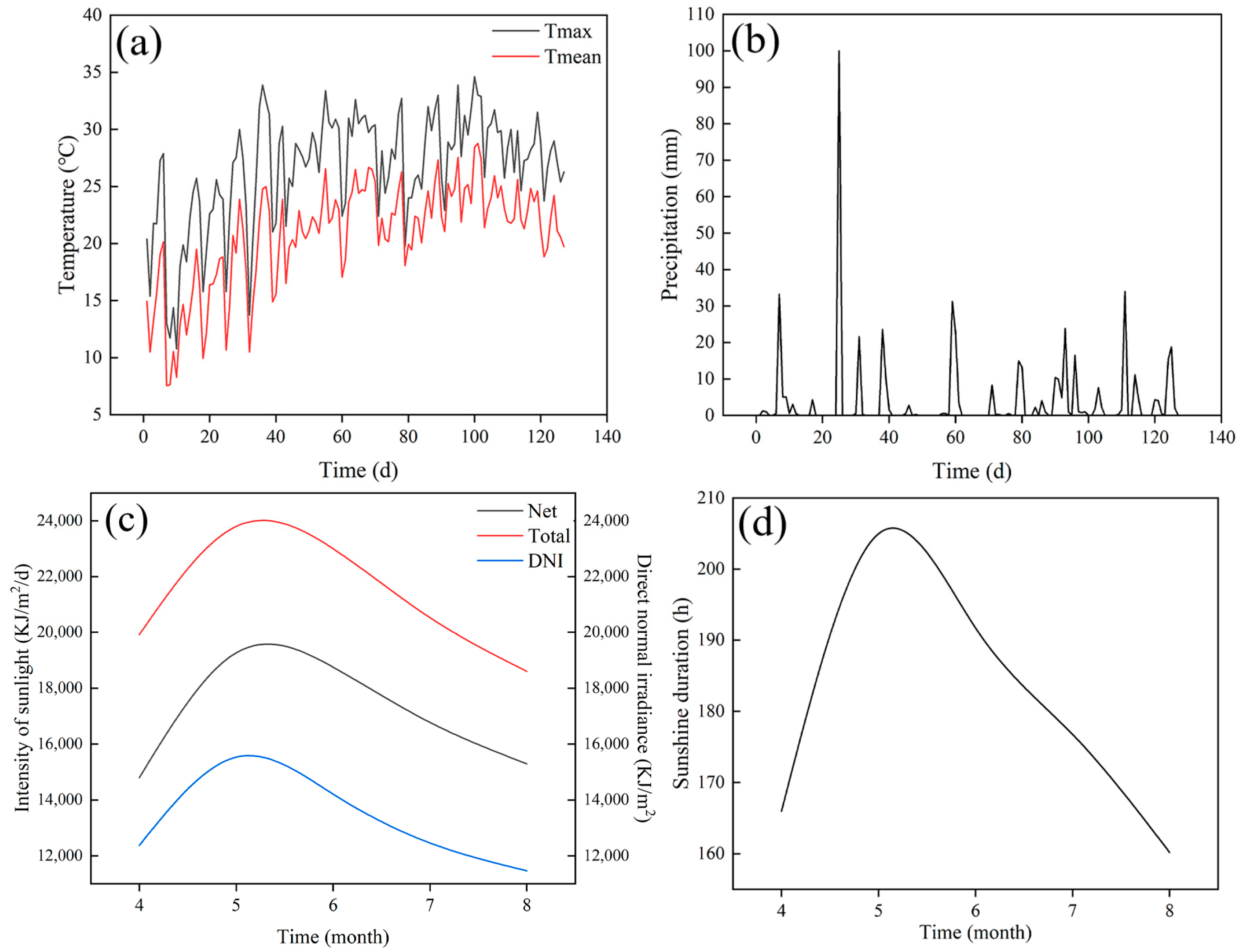
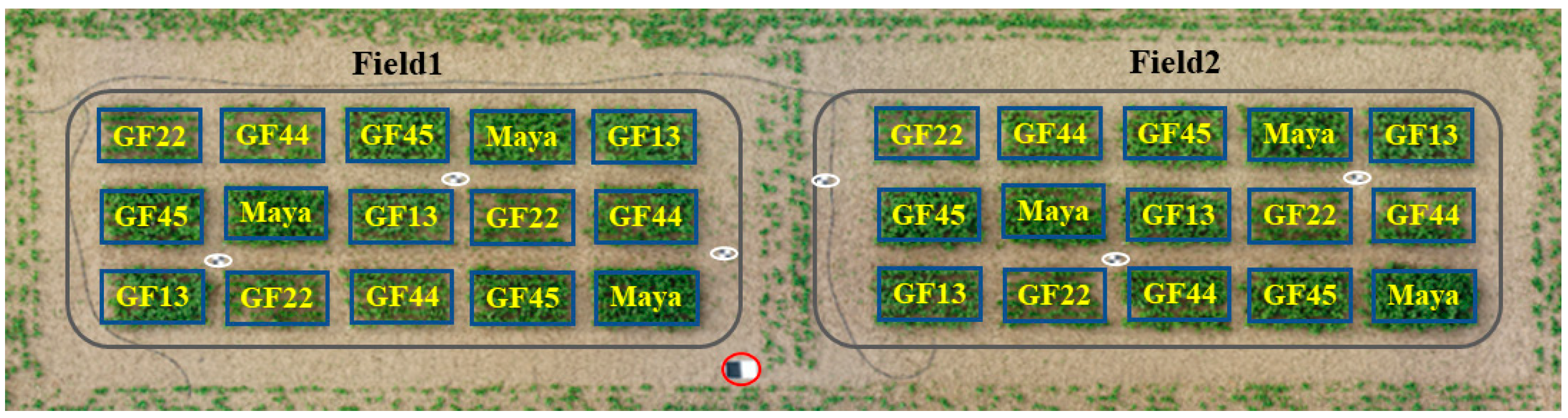
2.1. Test Site

The study was conducted at the Guyuan Experimental Station, which is affiliated with the Institute of Crop Sciences, Chinese Academy of Agricultural Sciences, in Zhangjiakou City, Hebei, China. The test site features a temperate arid and semi-arid climate, which is the transition climate between temperate forest and temperate desert. The average annual temperature was 1.6 °C, and the site was cold in the winter season and hot in the summer season. The annual precipitation is 426 mm, and the average annual frost-free period is 117 days. Detailed environmental conditions (temperature, precipitation, intensity of sunlight, and duration of sunshine) related to the faba bean growth periods were obtained from the weather bureau (Figure 1).
The trials began on 18 April 2019. The test site was divided into 2 experiment parts, and each part had 15 plots. Five faba bean varieties (GF13, GF22, GF44, GF45, and Maya) were tested, all of which were obtained from the Institute of Crop Sciences. The experiment was a completely randomized design with three replicates, and the varieties in the left and right experimental parts were arranged in the same manner. Each plot comprised six rows, and each row comprised 40 planted seeds. The specific arrangement results are shown in Figure 2. No fertilizer was applied, and weeding was conducted on demand during the test. Moreover, to improve the accuracy of subsequent image stitching, ground control points (GCPs) were evenly distributed across the whole field (Figure 2).

2.2. Data Collection

2.2.1. Collection of Ground Data

The ground data collected were mainly yield data, which were collected on 22 August 2019. The dry weight of all beans harvested in each plot was used for yield measurement.

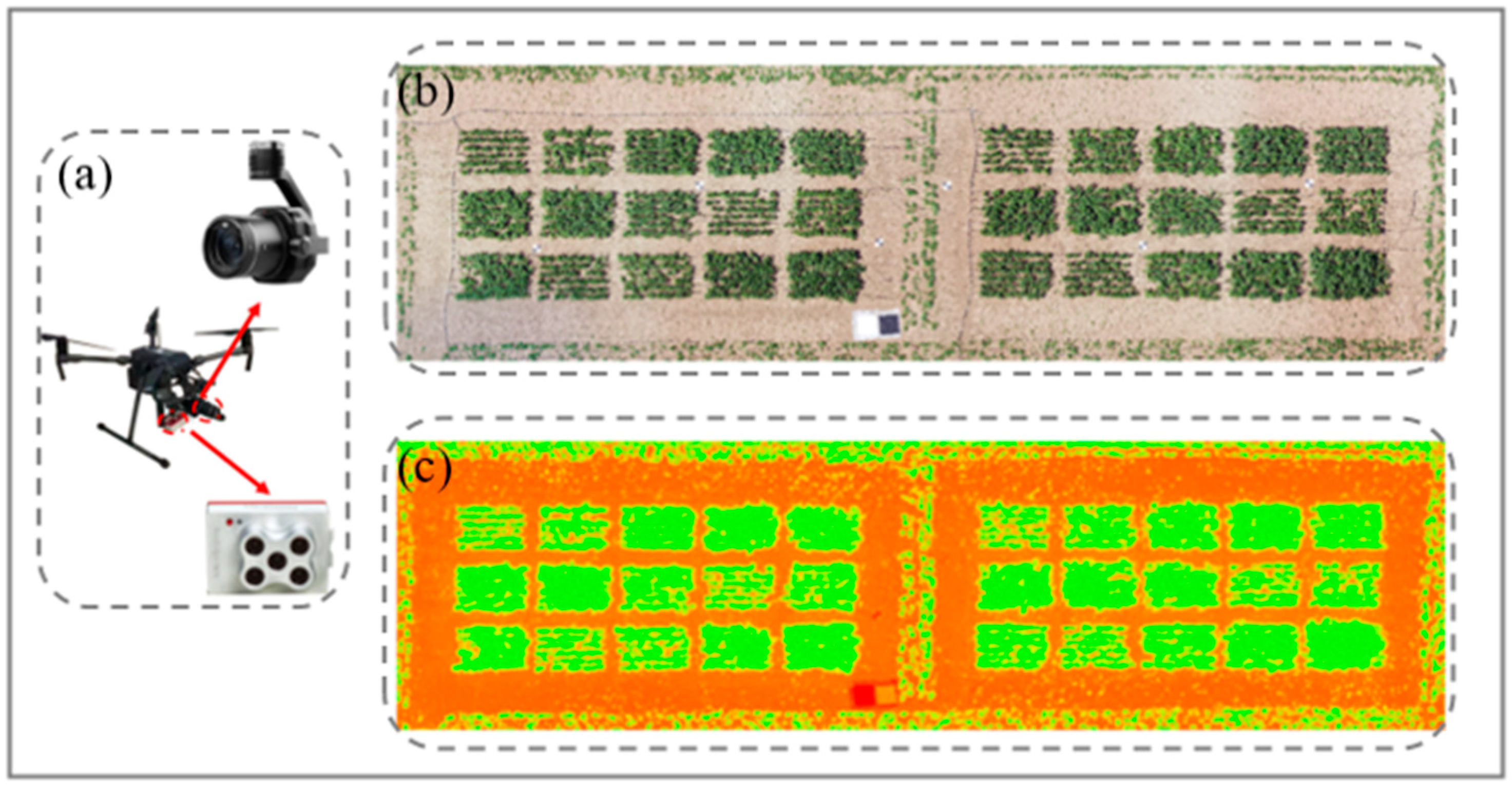
2.2.2. UAV Configuration

The UAV DJI Matrice 210 (SZ DJI Technology Co, Shenzhen, China; Figure 3) was applied to this study. It was equipped with an RGB sensor and a RedEdge-MX sensor. The RGB sensor was a 24 Megapixel DJI Zenmuse X7 camera (support output of up to 6 K/30 fps and 3.9 K/59.94 fps RAW), with dimensions of 151 mm × 108 mm × 132 mm. The RedEdge-MX sensor weighed about 232 g and contained five bands: blue (B: 475 nm); green (G: 560 nm); red (R: 668 nm); red-edge (RE: 717 nm); and near-infrared (N: 840 nm), with a resolution of 1280 × 960.

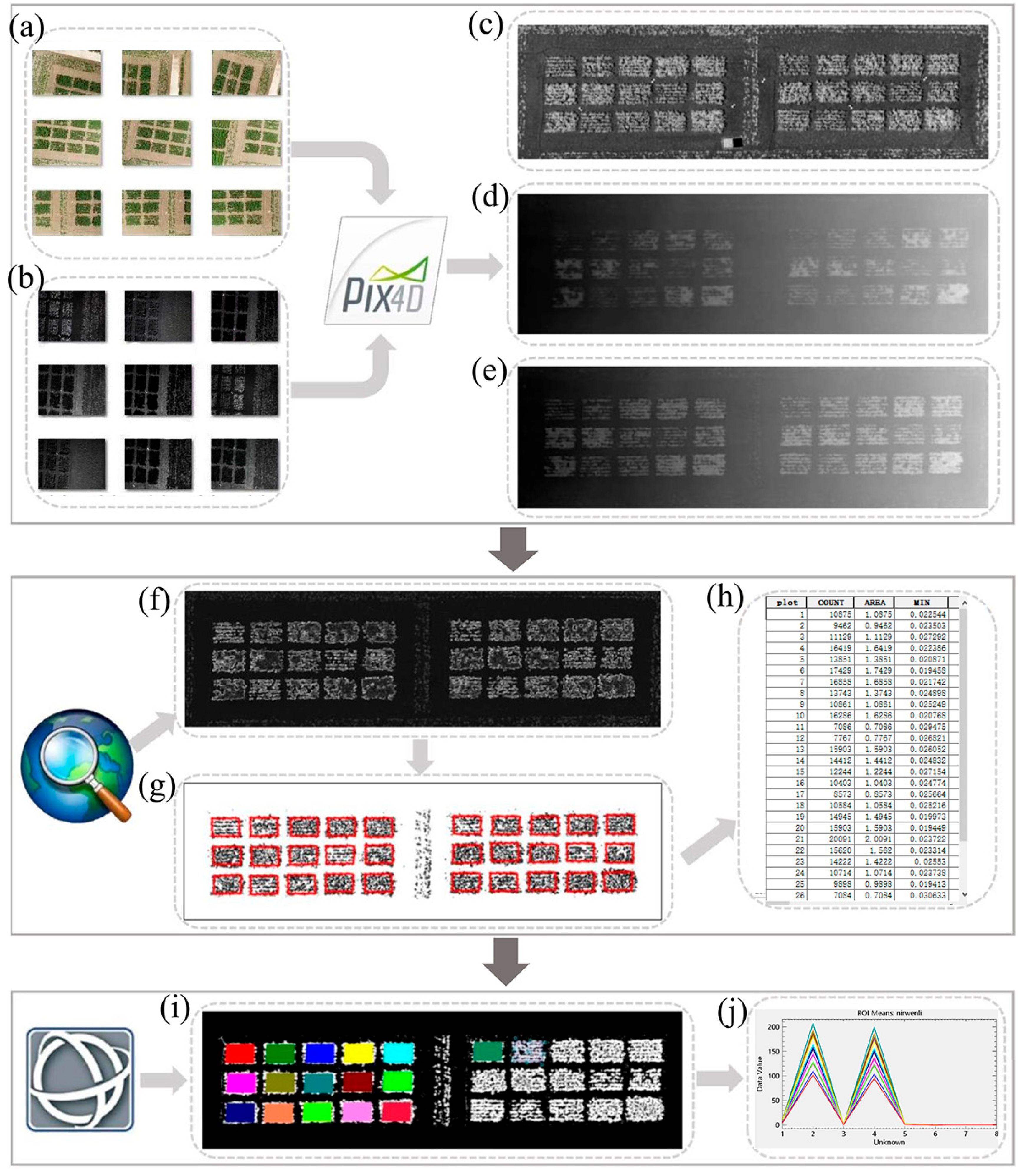
2.2.3. Acquisition and Processing of UAV-Based Data

To ensure the accuracy of data, we selected data for weather conditions without wind and cloud, and the UAV flew at a low speed, with an altitude of 25 m. For the RGB image collection, the flight planning parameters for the UAV imaging system included forward and side overlaps of 85% and 80%, respectively, while for the MS image collection, the forward and side overlaps were 80% and 75%, respectively. UAV data were collected for three dates: 17 June 2019 (S1), 12 July 2019 (S2), and 12 August 2019 (S3).
The UAV data were mainly processed in two steps: (1) mosaicking of UAV imagery; (2) extracting of UAV data. The simplified UAV-based data processing procedure is illustrated in Figure 4, and the specific steps are as follows. Because a large number of RGB images was obtained and a single image accounted for small coverage, mosaicking multiple images into a complete image for subsequent image processing and data extraction was vital. The UAV aerial RGB images were split using Pix4DMapper (Pix4D SA, Lausanne, Switzerland) via the following steps: Add photos; Test Quality; Build Dense Cloud; Build Mesh; Build Texture; Generate Digital Surface Model (DSM); Generate Digital Terrain Model (DTM); Build Orthomosaic. Then, the images were output in the TIFF format [25]. The UAV data were extracted using ENVI 5.3 (Exelis Visual Information Solutions, Inc., Boulder, CO, USA) and ArcMap 10.5 (Environmental Systems Research Institute, Inc., Redlands, CA, USA). The RGB images were preprocessed in ArcMap 10.5, and the steps included picture calibration, picture cropping, background removal, plant area selection, field canopy coverage (CC) extraction, and the extraction of other spectral information. Texture information was extracted using ENVI 5.3. The preprocessing workflow in ENVI 5.3 was as follows: first, the “co-occurrence” tool was adopted to calculate the pictures after background removal; then, the regions of interest were selected; and the texture information was output.
The stitching procedure of MS images was different from that of the RGB images. The reflectance was calibrated using a calibrated carpet (Figure 3). However, the imagery mosaicking and data extraction methods were the same as those for the RGB images and, thus, are not repeated here.
In addition, we inserted the DSM and DTM generated in Pix4DMapper into the software ArcMap 10.5, ran Equation (1) with a raster calculator to obtain the crop surface model (CSM), and then used tools (such as “Spatial Analyst and Spatial Analysis”) in ArcMap 10.5 to extract plant height data and select the maximum plant height of each plot selected for subsequent data processing. Equation (1) is expressed as
CSM = DSM − DTM

2.3. Vegetation Indices

The vegetation index can reflect the growth conditions of crops so that the crop phenotype information can be obtained according to spectral reflectance. Twenty-three vegetation indices obtained from RGB and MS cameras were used for faba bean yield estimation, which contains 8 RGB-related indices and 15 MS-related indices. The detailed equations are shown in Table 1.

2.4. ML Algorithms

In this study, four widely used ML methods, including SVM [44], RR [45], PLS [46], and KNN [47], were used to construct the yield estimation models.
SVM is a popular classification and statistical computing method developed by Vapnik and based on the statistical learning theory [48]. SVM can map input vectors to a high-dimensional space to create decision boundaries. Additionally, it can transform highly nonlinear data into linearly differentiable data using kernel functions. Thus, the advantages of SVM are reflected in its applicability under a small sample size, compatibility with high- and low-dimensionality data problems, and nonlinearity [49,50].
RR is a validated linear regression method developed by Tikhonov in 1943 and promoted by Hoerl and Kennard in 1970 [51,52]. RR is essentially a modified least squares estimation method that obtains more realistic and reliable regression coefficients at the expense of losing some information by giving up the unbiased nature of least squares [13]. RR is more suitable for the case of small training samples or feature correlation, which can effectively solve the problem of multicollinearity to ensure estimation accuracy [53].
PLS is a multivariate statistical method that was widely used in regression analysis [54]. It is characterized by the minimization of the autocorrelation effect between wavelengths, allowing for the effective solving of the multi-colinearity problem and the building of linear regression models [55].
KNN is a commonly used supervised learning algorithm capable of classification and regression tasks [56]. In the training phase, the samples are saved with zero training time overhead and then processed when the test samples are received. The training observation Zi affects the estimation only when Zi (Z denotes a sample of i observations drawn from the total) is one of the k-nearest neighbors of the target observation; therefore, the KNN estimation is highly stable [47]. Overall, the model is characterized by short time consumption, high accuracy, and high stability.

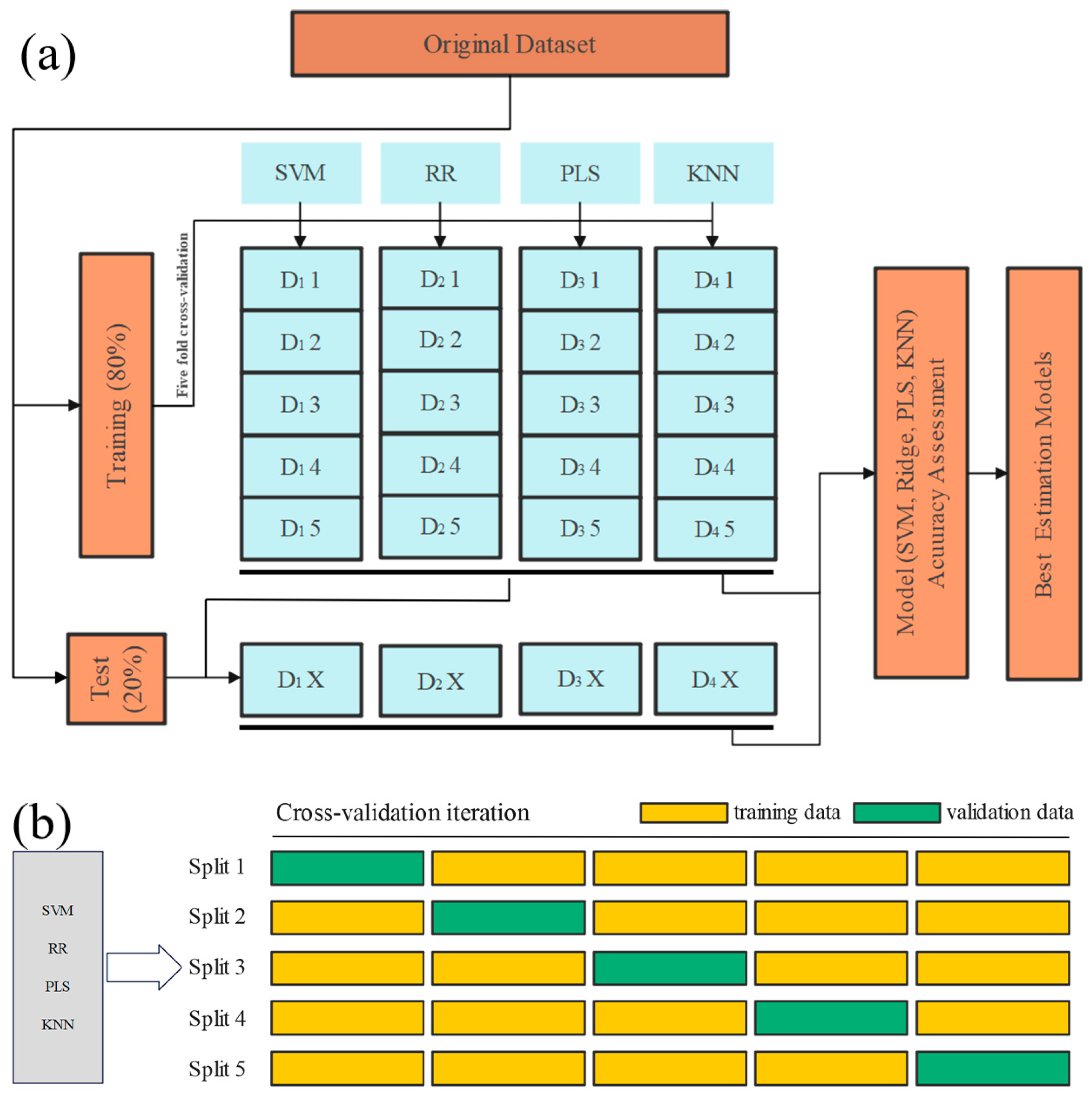
2.5. Model Construction and Evaluation

2.5.1. Model Construction

The data analysis and modeling were performed with the package “classification and regression training (caret)” in software R 4.2.3 (Lucent Technologies, Murray Hill, NJ, USA). The modeling process is summarized in Figure 5.
To avoid the overfitting of the ML models and to make full use of all training sets for model training and testing, each of the ML methods was used to do five-fold cross-validation (Figure 5b). The training data were randomly and evenly divided into five equal sets, four of which were used for model training and the remaining one for testing. Five folds were repeatedly iterated, with one-fifth of the data set selected each time as the test set and the other data sets aggregated as the training sets, after which the model was trained on the test set, tested according to the trained model, and the accuracy calculated. The final accuracy was obtained by averaging the accuracies of the five times. This process was repeated 10 times during the model construction to increase the stability of the model using the “repeats” function.

2.5.2. Model Evaluation

The accuracy of the model was evaluated using the coefficient of determination (R2), root-mean-square error (RMSE), and normalized root-mean-square error (NRMSE). R2 was mainly used to measure the fitting degree of the model. An R2 closer to 1 indicates a higher fitting degree. The estimation error of the model was measured using RMSE and NRMSE. The smaller the RMSE and NRMSE values, the smaller the estimation error of the model. The final results in this study were the average of five “for” loops. The calculation equations for these parameters are as follows:
R 2 = 1 i = 1 n ( x i y i ) 2 i = 1 n ( x i y ¯ ) 2
RMSE = i = 1 n ( x i y i ) 2 n
NRMSE = i = 1 n ( x i y i ) 2 n y ¯ × 100 %
where x i is the measured yield of faba bean; y i is the yield estimated by the model; y ¯ is the mean of the measured yield, and n is the total number of testing samples.

3. Results

3.1. Faba Bean Yield Estimation for the Optimal Single-Growth Period

To explore the influence of different growth periods on the yield estimation results, four algorithms were grouped into the same box, and the estimation accuracies for the different growth periods were compared. The specific evaluation metrics of the models are shown in Table 2. The average R2 of the S2 model (R2 = 0.563) based on MS sensor data was 0.089 and 0.045 higher than those of the S1 and S3 models, respectively (Figure 6a); the average R2 of the S2 model based on RGB sensor data (R2 = 0.616) was 0.111 and 0.104 higher than those of the S1 and S3 models, respectively. For the dual-sensor data (RGB + MS), the average R2 of the S2 model (R2 = 0.682) was 0.157 and 0.056 higher than those of the S1 (R2 = 0.525) and S3 (R2 = 0.626) models, respectively. Figure 6b,c reflected the errors of the model, and the model constructed according to the S2 period yielded considerably fewer errors for all of the different sensors (RGB, MS, and RGB + MS) of inputting data. In general, the S2 model yielded the best estimation results, followed by the S3 model.

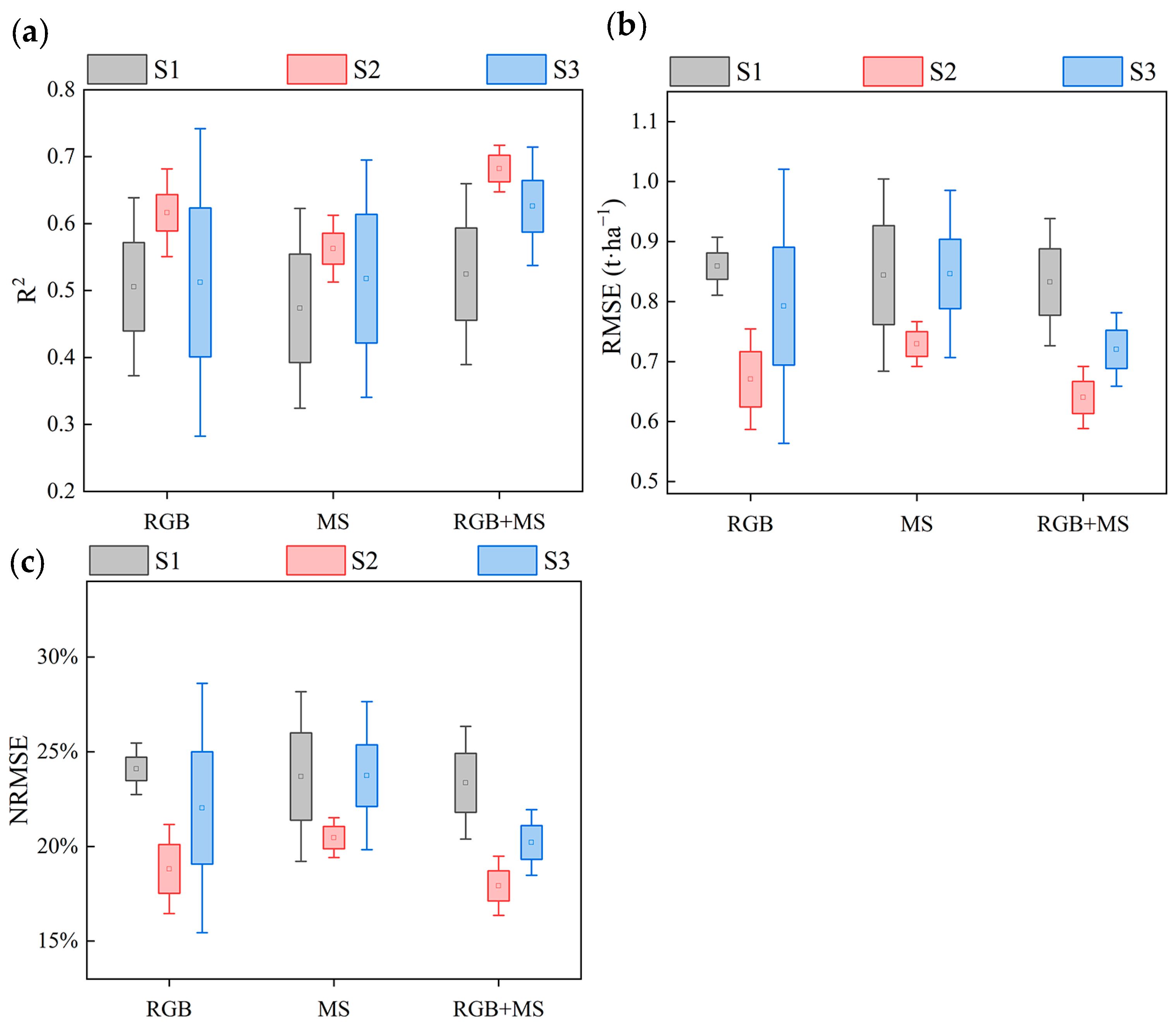
3.2. Faba Bean Yield Estimation for Optimal Sensor

Two kinds of sensor (RGB, MS) data and their fusion were used for yield estimation. Given that the S2 model exhibited the best highest accuracy, relevant S2 data were selected for model construction (Figure 7), and the evaluation metrics of the model were shown in Table 2. The RGB + MS-based model exhibited the highest correlation; the R2 values of the four ML algorithms were between 0.661 and 0.707, which corresponded to satisfactory estimation results. The total R2 values of the model constructed with single RGB and MS sensor data were 0.264 and 0.479 lower than those of the RGB + MS-based model, respectively. Moreover, the model based on the RGB + MS fusion data yielded fewer errors than those based on single-sensor data. The total RMSE values of the RGB + MS-based model were 0.121 and 0.356 t·ha−1 lower than those of the RGB- and MS-based models, respectively, and the total NRMSE values of the RGB + MS-based model were 3.577% and 10.183% lower than those of the RGB- and MS-models, respectively. Overall, the RGB + MS model exhibited the highest yield estimation accuracy in most cases, followed by the RGB-based model.

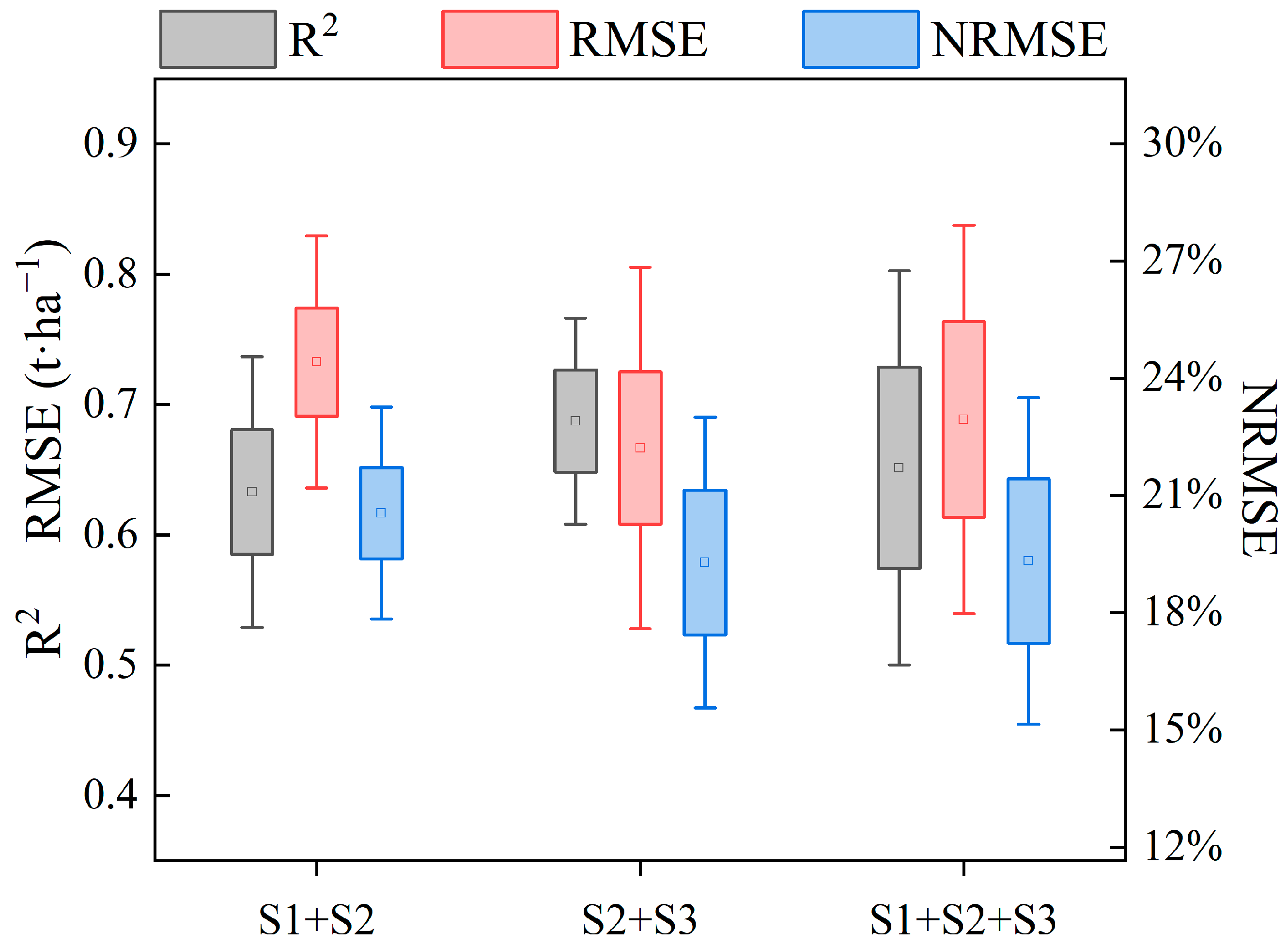
3.3. Faba Bean Yield Estimation for Multiple Growth Periods

To the best of our knowledge, all of the previous studies adopted single-period data and did not combine data from multiple growth periods to estimate faba bean yield. To evaluate the yield estimation accuracies of models based on the data of multiple growth periods, we constructed models based on data from multiple growth periods using the same model structure, parameters, and fused dual-sensor data used in the single-growth-period models (the RGB + MS data were used because the RGB + MS model exhibited the highest accuracy for the single-growth period). We compared the correlations and errors obtained by the models based on different growth period combinations. The results are shown in Table 3 and Figure 8. The model based on S2 + S3 data exhibited the highest estimation accuracy, with verification results (mean) of R2 = 0.687, RMSE = 0.667 t·ha−1, and NRMSE = 18.705%, followed by the model based on S1 + S2 + S3 data (R2 = 0.651, RMSE = 0.689 t·ha−1, and NRMSE = 19.325%). The model based on S1 + S2 yielded the lowest estimation accuracy (R2 = 0.633, RMSE = 0.733 t·ha−1, and NRMSE = 20.551%); the low-accuracy results are attributable to the relatively inaccurate data for the S1 period, which resulted in data redundancy, and consequently, the estimation accuracy of the model constructed according to the fused data of the three growth periods data was lower than that of the S2 + S3-based model [57].

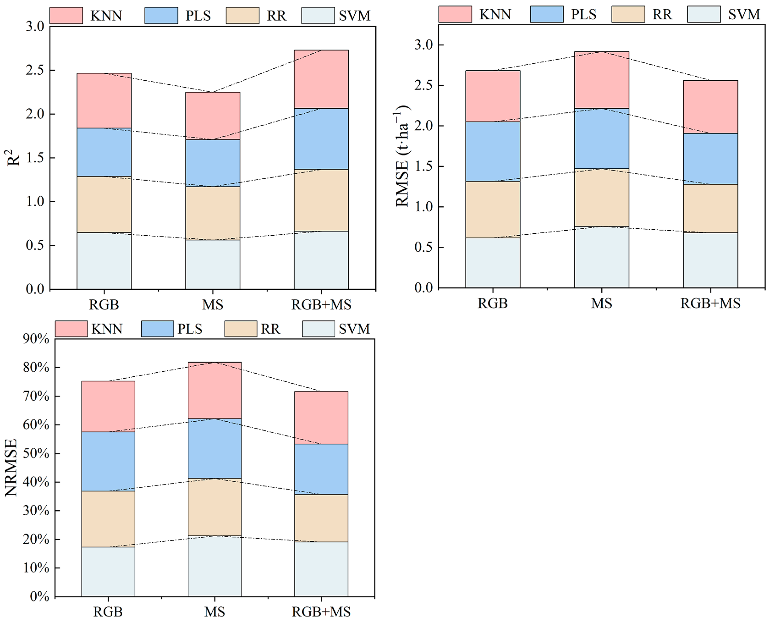
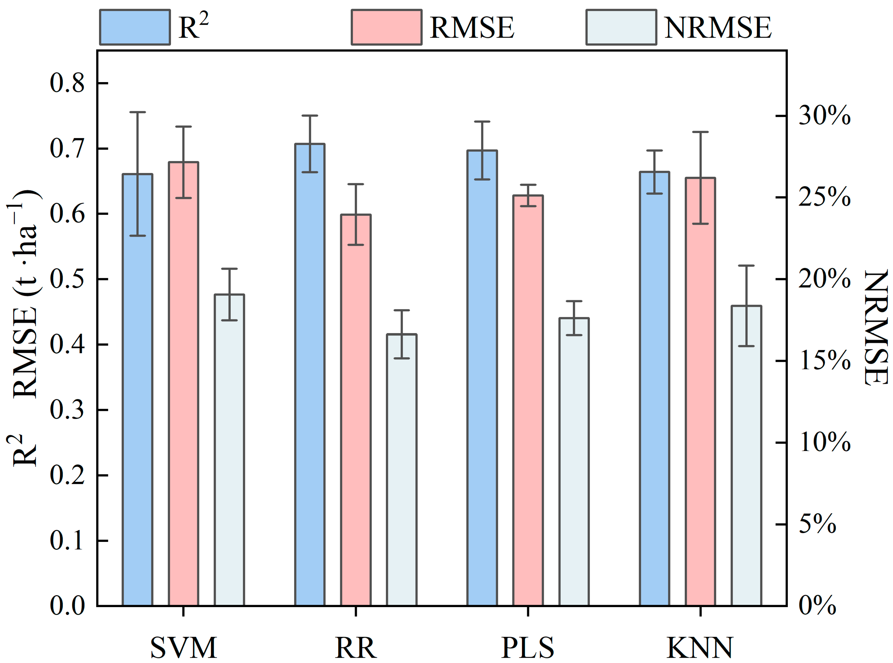
3.4. Optimal ML Algorithm for Faba Bean Yield Estimation

The data based on the S2 period and RGB + MS fusion were confirmed to be optimal. The optimal data were used to construct the faba bean yield estimation model. To test the accuracies of different ML algorithms, different yield estimation models were constructed using four algorithms, and the model estimation accuracies were compared and analyzed. The performances of the various ML algorithms on faba bean yield estimation were considerably different, and the specific results are shown in Figure 9, and the specific assessment metrics are shown in Figure 2. The R2 values of SVM, PLS, and KNN were 0.046, 0.010, and 0.043 lower than those of the RR model, respectively, which means that the RR model exhibited a higher correlation degree. The RMSE values of SVM, PLS, and KNN were 0.080, 0.029, and 0.056 t·ha−1 higher than those of the RR model, respectively, and the NRMSE values of SVM, PLS, and KNN were 2.436%, 0.989%, and 1.747% higher than those of the RR model, respectively, which indicated that the RR model exhibited the fewest errors. Overall, RR was the best algorithm for the yield estimation model, followed by PLS.

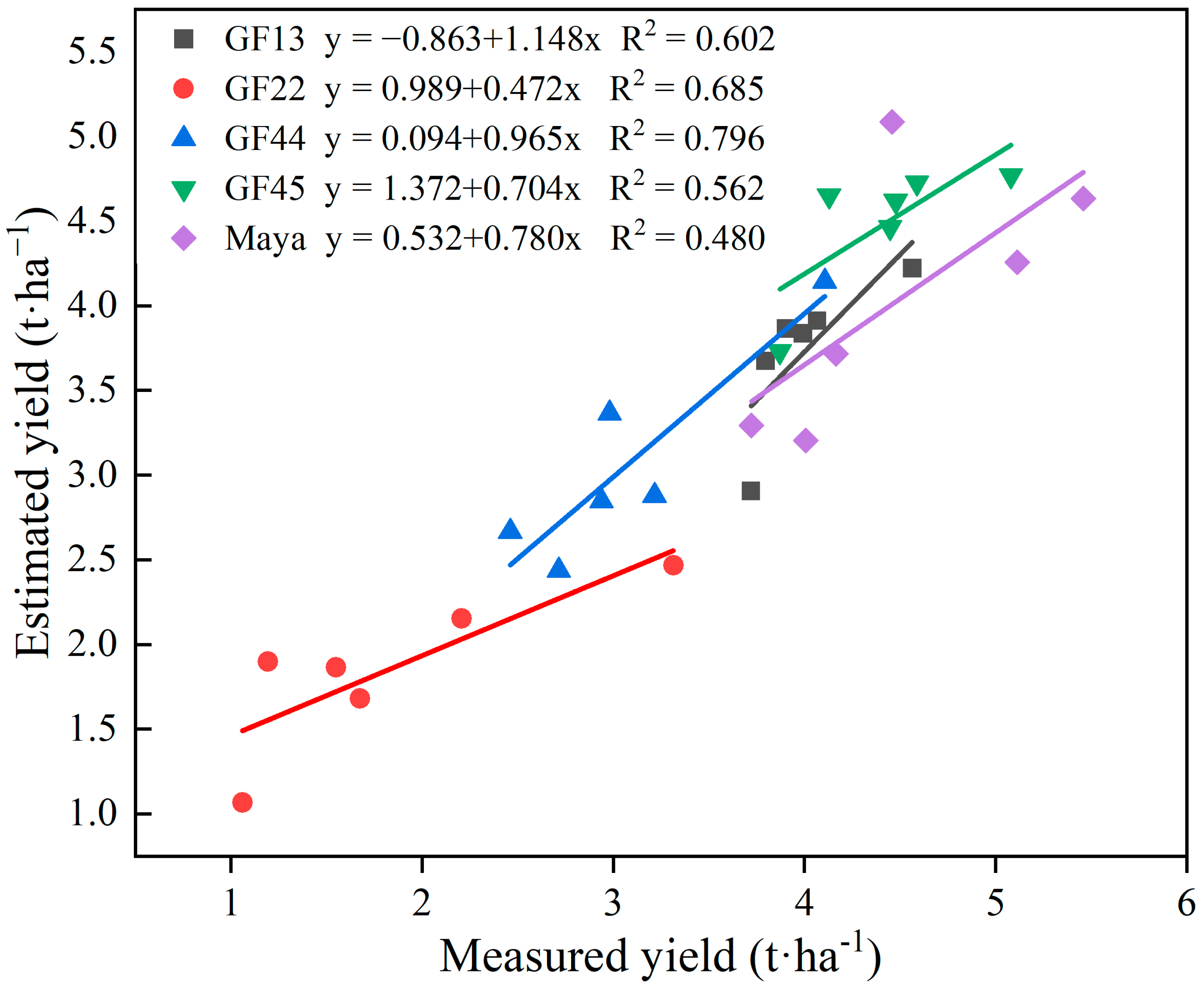
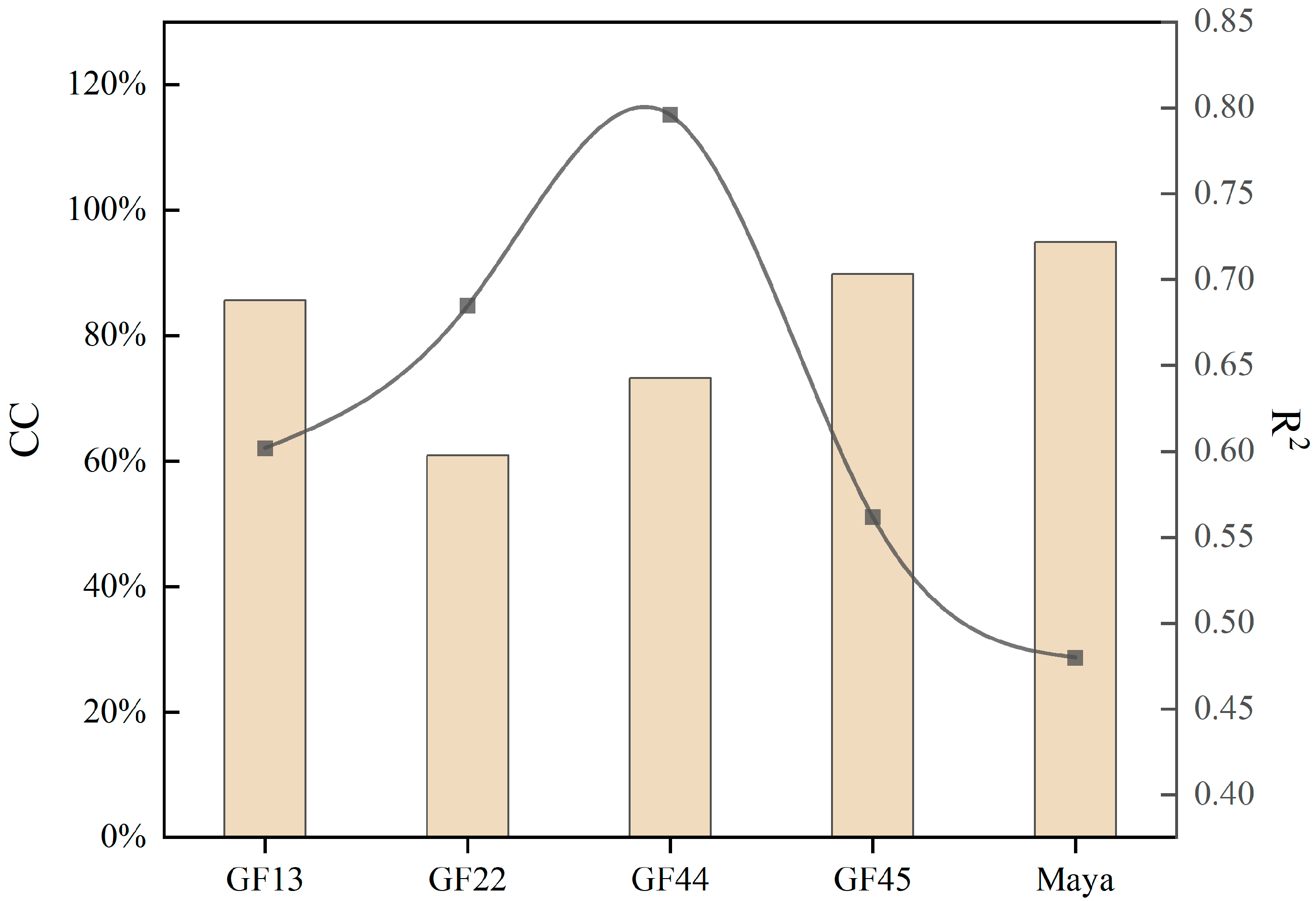
3.5. Influence of Faba Bean Variety on Yield Estimation Model

To test the accuracy of the RR model, the correlations and linear fitting degrees between estimated and measured yields for different faba bean varieties were compared (Figure 10). The R2 values of GF13, GF22, GF44, GF45, and Maya were 0.602, 0.685, 0.796, 0.562, and 0.480, respectively, which meant that the RR model exhibited an acceptable estimation accuracy for the different varieties. However, the effect of Maya yield estimation was worse than those of the other varieties (GF13, GF22, GF44, and GF45). The lower Maya yield estimation accuracy may be attributable to the higher plant density of the plot and the higher overlap of the faba bean plants, which agrees well with the results of the previous research on annotated and detected plants [58].

4. Discussion

Early yield estimation could help guide breeding decisions and make the most efficient use of limited land resources. In recent years, with the need for agricultural production and the gradual emergence of UAV-based remote sensing [59], UAV-based remote sensing data have been increasingly used for estimating the yields of staple crops (such as maize [60] and wheat [61]); however, studies on the use of remote sensing data for estimating the phenotypic parameters of faba beans are few, and only two relevant articles have been published [49,62]. Different factors influence the accuracy of faba bean yield estimation models, including the growth period, the growth period data type (single or combined), the adopted ML algorithm, crop varieties, and sensor types (single or combined). These factors were explored in this study.

4.1. The Effects of Growth Periods Data on Yield Estimation

The growth period serves as both a developmental landmark and a trigger for collecting phenotype data [63,64]. Therefore, several studies of plant phenotypes have considered the growth period. In the current study, three growth periods were considered: 17 June 2019 (S1), 12 July 2019 (S2), and 12 August 2019 (S3). The data for each growth period were used as a group of variables to train the estimation model. The S1, S2, and S3 models differed in their D-value, which suggested that the accuracy of the faba bean yield estimation based on UAV data depends on the plant growth period, and the accuracy of the estimations of the S2 model was the highest. For the dual-sensor-based model, the mean estimation accuracy of S2 is R2 = 0.682, RMSE = 0.640 t·ha−1, NRMSE = 17.919%; these metrics are better than that of S1 (R2 = 0.524, RMSE = 0.833 t·ha−1, NRMSE = 23.364%) and S3 (R2 = 0.626, RMSE = 0.720 t·ha−1, NRMSE = 20.212%). These results are partly consistent with those of a recent study by Liu [16] and Oehme [64]. In addition, only a few phenotypic studies have combined multiple growth periods, despite the advantages of combined data. In the current study, the data for different growth periods were combined to estimate yield. The models based on the three growth periods exhibited a lower accuracy than the S2 + S3-based model (Figure 8), indicating that the adoption of a reasonable sample size and data combination resulted in the highest estimation accuracy, whereas the adoption of an excessive sample size might reduce the accuracy of a model owing to data redundancy [57,65].

4.2. Contribution of Individual Sensor Data and Dual-Sensor Data Fusion to Yield Estimation

Previous studies which used single-sensor data were used to obtain crop phenotypic parameters. In the current study, the use of RGB features resulted in a higher faba bean yield estimation accuracy than the use of MS features, possibly because RGB images have a higher spatial resolution than MS images, and the information on plant height extracted from RGB images has positive effects on yield estimation [14]. Some studies have also proved that the height information extracted by RGB images is highly related to the yield information, and it can effectively improve the accuracy of the yield estimation model when combined with the vegetation indices [49,66,67].
However, this study showed that dual-sensor data fusion resulted in a higher value of R2 than the use of single-sensor data for all of the four considered ML algorithms. Previous studies have also confirmed that coupling spectra with the characteristic variables of other sensors could improve the model estimation accuracy [68,69], which probably explains why multiple information, such as unique spectral, structural, and height, contributes to crop yield estimation complementarily [14,17]. Ji et al. [49,62] used single-sensor data to construct a faba bean yield estimation model, but in the current study, dual-sensor data was used in the yield estimation, which also had relatively better performance.

4.3. Effects of Different ML Algorithms on Yield Estimation Model

According to previous studies, many ML models (such as RR, RF, SVM, and Cubist) have been successfully applied as tools for early crop phenotype estimation [13,14,70,71]. In the current study, four algorithms (SVM, RR, KNN, and PLS) were used to construct the yield estimation models. The RR model was the best-performing model under all conditions for the selected growth periods; the PLS model lagged behind the RR model in terms of prediction accuracy under most conditions. These results are also partially consistent with the results of Fei et al. [13], who found that RR worked better in fixing the training dataset and showed a higher estimation accuracy. Other studies have also demonstrated the high accuracy and robustness of the RR model under most modeling conditions [71,72]. The reason for the higher accuracy of RR is probably because RR can perform regularization for the coefficients of the model, that is, restrain the sum of squared coefficients, which smoothens the coefficients of the model to reduce the variance and improves the estimation accuracy [13,72]. However, in the current study, the SVM- and KNN-based models exhibited low accuracies, which suggested that these ML algorithms might not be suitable for the construction of faba bean yield estimation models in this study. Furthermore, other studies have shown that ensemble learning-based estimation models could further improve estimation accuracy [13,14]. Therefore, the impact of ensemble learning on the accuracy of faba bean yield estimation should be explored.

4.4. The Effects of Faba Bean Variety and Growth on Yield Estimation

Figure 10 shows that the R2 values of GF13, GF22, GF44, GF45, and Maya were 0.602, 0.685, 0.796, 0.562, and 0.480, respectively. Crop variety considerably influenced the yield estimation model [17]. The estimation results of different varieties were similar to the results of a previous study, which reported that the grain yield estimations were different for different varieties, attributable to the differences in growth periods, growth characteristics, and other phenotypic characteristics among different varieties [16,73].
Crop growth characteristics, including density, overlap, CC, and lodging conditions, considerably influenced the accuracy of the phenotype estimation model with canopy [58,74]. CC is a common structural characteristic applied in both remote sensing and ecological studies [74,75]. A certain correlation existed between CC and yield estimation accuracy. The models exhibited the highest estimation accuracy under a CC of 61–73% (Figure 11). Under a CC of ~73%, the model achieved the highest estimation accuracy, which proved that a correlation existed between CC and the model estimation accuracy.

4.5. Limitations and Implications

UAV-based RGB and MS images on the faba bean canopy were collected to estimate yield. The dual-sensor combined data were used to estimate the faba bean yield, which resulted in a higher estimation accuracy than a single sensor. Additionally, the reasonable combination of data for multiple growth periods improved the estimation accuracy. These two methods (sensor data fusion and growth period data fusion) will become the main research directions for crop modeling in the future [14]. Additionally, this study used small sample data for model construction, which has some instability but can achieve the effect of improving the stability of the model after dozens of cross-validations. The crop growth model with small sample data has the advantages of low consumption, flexibility, efficiency, compatibility, and other advantages that large experimental sample data models do not have [57,76].
Hence, future research should consider adding types of sensors (such as laser radar and thermal infrared sensors) and the number of growth periods to obtain more accurate models. Moreover, in addition to combining data from different sensors and growth periods, ensemble learning should be considered in future research. Additionally, future research will be conducted to compare crop model studies with small and large sample data to explore the impact on crop models, such as on the accuracy and stability of the models.

5. Conclusions

This study explored the potential of combining RGB and MS sensor data and the data of different growth periods for the construction of faba bean yield estimation models, and the effects of different ML algorithms and varieties on the model accuracy were examined. The main conclusions are as follows:
(1)
The effects of growth periods were explored in this study. The model based on S2 (12 July 2019) exhibited a higher estimation accuracy than the models based on the other single-growth periods. The model based on the combination of S2 and S3 (12 August 2019) exhibited a higher estimation accuracy than the models based on the other combined growth periods;
(2)
The models based on fused dual-sensor data yielded higher estimation accuracies than the models based on single-sensor data;
(3)
The comparison of four ML algorithms (SVM, RR, PLS, and KNN) showed that RR resulted in the highest yield estimation accuracy, followed by PLS; the SVM- and KNN-based models exhibited the worst performances.
The research contributes two innovative ideas to the yield estimation of faba beans and, thus, can provide a reference for the follow-up research on faba beans and other crops.

Author Contributions

Y.C. wrote the manuscript; Y.J. designed the study, and both analyzed the data; T.Y. and X.Z. directed the trial and provided the main idea; R.L. and W.L. participated in data collection; Z.L. helped with image processing; Y.L. provided comments and suggestions to improve the manuscript. All authors have read and agreed to the published version of the manuscript.

Funding

This study was funded by the China Agriculture Research System of MOF and MARA-Food Legumes (CARS-08), the Project of accurate identification of faba bean germplasm resources, Agricultural Science and Technology Innovation Program in CAAS, and the National Crop Genebank project from the Ministry of Science and Technology of China (NCGRC-2023-7).

Data Availability Statement

The original contributions presented in this study are included in the article; further inquiries can be directed to the corresponding authors.

Acknowledgments

We would like to thank all the teachers who have contributed to this article.

Conflicts of Interest

The authors declare that the research was conducted in the absence of any commercial or financial relationships that could be construed as a potential conflict of interest.

References

  1. Abete, I.; Romaguera, D.; Vieira, A.R.; Lopez, M.A.; Norat, T. Association between total, processed, red and white meat consumption and all-cause, CVD and IHD mortality: A meta-analysis of cohort studies. Br. J. Nutr. 2014, 112, 762–775. [Google Scholar] [CrossRef] [PubMed] [Green Version]
  2. Chen, Z.; Franco, O.H.; Lamballais, S.; Ikram, M.A.; Schoufour, J.D.; Muka, T.; Voortman, T. Associations of specific dietary protein with longitudinal insulin resistance, prediabetes and type 2 diabetes: The Rotterdam: The Rotterdam Study. Clin. Nutr. 2020, 39, 242–249. [Google Scholar] [CrossRef] [PubMed]
  3. Farvid, M.S.; Sidahmed, E.; Spence, N.D.; Angua, M.K.; Rosner, B.A.; Barnett, J.B. Consumption of red meat and processed meat and cancer incidence: A systematic review and meta-analysis of prospective studies. Eur. J. Epidemiol. 2021, 36, 937–951. [Google Scholar] [CrossRef] [PubMed]
  4. Martineau-Côté, D.; Achouri, A.; Karboune, S.; L’Hocine, L. Faba Bean: An Untapped Source of Quality Plant Proteins and Bio-actives. Nutrients 2022, 14, 1541. [Google Scholar] [CrossRef]
  5. Burud, I.; Lange, G.; Lillemo, M.; Bleken, E.; Grimstad, L.; From, P.J. Exploring Robots and UAVs as Phenotyping Tools in Plant Breeding. IFAC-Pap. 2017, 50, 11479–11484. [Google Scholar] [CrossRef]
  6. Shafiee, S.; Lied, L.M.; Burud, I.; Dieseth, J.A.; Alsheikh, M.; Lillemo, M. Sequential forward selection and support vector regression in comparison to LASSO regression for spring wheat yield prediction based on UAV imagery. Comput. Electron. Agric. 2021, 183, 106036. [Google Scholar] [CrossRef]
  7. Peñuelas, J.; Gamon, J.; Fredeen, A.; Merino, J.Á.; Field, C.B. Reflectance indices associated with physiological changes in nitrogen- and water-limited sunflower leaves. Remote Sens. Environ. 1994, 48, 135–146. [Google Scholar] [CrossRef]
  8. Marino, B.D.; Geissler, P.; O’connell, B.; Dieter, N.; Burgess, T.; Roberts, C.; Lunine, J. Multispectral imaging of vegetation at Biosphere 2. Ecol. Eng. 1999, 13, 321–331. [Google Scholar] [CrossRef]
  9. Feng, L.; Zhang, Z.; Ma, Y.; Du, Q.; Williams, P.; Drewry, J.; Luck, B. Alfalfa Yield Prediction Using UAV-Based Hyperspectral Imagery and Ensemble Learning. Remote Sens. 2020, 12, 2028. [Google Scholar] [CrossRef]
  10. Bhadra, S.; Sagan, V.; Maimaitijiang, M.; Maimaitiyiming, M.; Newcomb, M.; Shakoor, N.; Mockler, T.C. Quantifying Leaf Chlorophyll Concentration of Sorghum from Hyperspectral Data Using Derivative Calculus and Machine Learning. Remote Sens. 2020, 12, 2082. [Google Scholar] [CrossRef]
  11. Feng, A.; Zhou, J.; Vories, E.D.; Sudduth, K.A.; Zhang, M. Yield estimation in cotton using UAV-based multi-sensor imagery. Biosyst. Eng. 2020, 193, 101–114. [Google Scholar] [CrossRef]
  12. Herrero-Huerta, M.; Rodriguez-Gonzalvez, P.; Rainey, K.M. Yield prediction by machine learning from UAS-based mulit-sensor data fusion in soybean. Plant Methods 2020, 16, 78. [Google Scholar] [CrossRef]
  13. Fei, S.; Hassan, M.A.; He, Z.; Chen, Z.; Shu, M.; Wang, J.; Li, C.; Xiao, Y. Assessment of Ensemble Learning to Predict Wheat Grain Yield Based on UAV-Multispectral Reflectance. Remote Sens. 2021, 13, 2338. [Google Scholar] [CrossRef]
  14. Fei, S.; Hassan, M.A.; Xiao, Y.; Su, X.; Chen, Z.; Cheng, Q.; Duan, F.; Chen, R.; Ma, Y. UAV-based multi-sensor data fusion and machine learning algorithm for yield prediction in wheat. Precis. Agric. 2023, 24, 187–212. [Google Scholar] [CrossRef]
  15. Sharma, L.K.; Bu, H.; Franzen, D.W.; Denton, A. Use of corn height measured with an acoustic sensor improves yield estimation with ground based active optical sensors. Comput. Electron. Agric. 2016, 124, 254–262. [Google Scholar] [CrossRef] [Green Version]
  16. Liu, S.; Jin, X.; Nie, C.; Wang, S.; Yu, X.; Cheng, M.; Shao, M.; Wang, Z.; Tuohuti, N.; Bai, Y.; et al. Estimating leaf area index using unmanned aerial vehicle data: Shallow vs. deep machine learning algorithms. Plant Physiol. 2021, 187, 1551–1576. [Google Scholar] [CrossRef]
  17. Maimaitijiang, M.; Sagan, V.; Sidike, P.; Hartling, S.; Esposito, F.; Fritschi, F.B. Soybean yield prediction from UAV using multimodal data fusion and deep learning. Remote Sens. Environ. 2020, 237, 111599. [Google Scholar] [CrossRef]
  18. Bendig, J.; Yu, K.; Aasen, H.; Bolten, A.; Bennertz, S.; Broscheit, J.; Gnyp, M.L.; Bareth, G. Combining UAV-based plant height from crop surface models, visible, and near infrared vegetation indices for biomass monitoring in barley. Int. J. Appl. Earth Obs. 2015, 39, 79–87. [Google Scholar] [CrossRef]
  19. Fu, P.; Meacham-Hensold, K.; Guan, K.; Bernacchi, C.J. Hyperspectral Leaf Reflectance as Proxy for Photosynthetic Capacities: An Ensemble Approach Based on Multiple Machine Learning Algorithms. Front. Plant Sci. 2019, 10, 730. [Google Scholar] [CrossRef]
  20. Jin, X.; Li, Z.; Feng, H.; Ren, Z.; Li, S. Deep neural network algorithm for estimating maize biomass based on simulated Sentinel 2A vegetation indices and leaf area index. Crop. J. 2020, 8, 87–97. [Google Scholar] [CrossRef]
  21. Matese, A.; Di Gennaro, S.F. Beyond the traditional NDVI index as a key factor to mainstream the use of UAV in precision viticulture. Sci. Rep. 2021, 11, 2721. [Google Scholar] [CrossRef]
  22. Yu, D.; Zha, Y.; Shi, L.; Jin, X.; Hu, S.; Yang, Q.; Huang, K.; Zeng, W. Improvement of sugarcane yield estimation by assimilating UAV-derived plant height observations. Eur. J. Agron. 2020, 121, 126159. [Google Scholar] [CrossRef]
  23. Zhang, Y.; Yang, Y.; Zhang, Q.; Duan, R.; Liu, J.; Qin, Y.; Wang, X. Toward Multi-Stage Phenotyping of Soybean with Multimodal UAV Sensor Data: A Comparison of Machine Learning Approaches for Leaf Area Index Estimation. Remote Sens. 2022, 15, 7. [Google Scholar] [CrossRef]
  24. Tunrayo, R.A.; Abush, T.A.; Godfree, C.; Fowobaje, K.R. Estimation of soybean grain yield from multispectral high-resolution UAV data with machine learning models in West Africa. Remote Sens. Appl. 2022, 27, 100782. [Google Scholar]
  25. Han, L.; Yang, G.; Dai, H.; Xu, B.; Yang, H.; Feng, H.; Li, Z.; Yang, X. Modeling maize above-ground biomass based on machine learning approaches using UAV remote-sensing data. Plant Methods 2019, 15, 10. [Google Scholar] [CrossRef] [Green Version]
  26. Tucker, C.J. Red and photographic infrared linear combinations for monitoring vegetation. Remote Sens. Environ. 1979, 8, 127–150. [Google Scholar] [CrossRef] [Green Version]
  27. Woebbecke, D.M.; Meyer, G.E.; Bargen, K.V.; Mortensen, D. Plant species identification, size, and enumeration using machine vision techniques on near-binary images. Opt. Agric. For. 1993, 1836, 208–219. [Google Scholar]
  28. Louhaichi, M.; Borman, M.M.; Johnson, D.E. Spatially located platform and aerial photography for documentation of grazing impacts on wheat. Geocarto Int. 2001, 16, 65–70. [Google Scholar] [CrossRef]
  29. Gitelson, A.A.; Kaufman, Y.J.; Stark, R.; Rundquist, D. Novel algorithms for remote estimation of vegetation fraction. Remote Sens. Environ. 2002, 80, 76–87. [Google Scholar] [CrossRef] [Green Version]
  30. Meyer, G.E.; Neto, J.C. Verification of color vegetation indices for automated crop imaging applications. Comput. Electron. Agric. 2008, 63, 282–293. [Google Scholar] [CrossRef]
  31. Woebbecke, D.M.; Meyer, G.E.; Bargen, K.V.; Mortensen, D.A. Color indices for weed identification under various soil, residue, and lighting conditions. Trans. ASAE 1994, 38, 259–269. [Google Scholar] [CrossRef]
  32. Gitelson, A.A.; Viña, A.; Ciganda, V.; Rundquist, D.C.; Arkebauer, T.J. Remote estimation of canopy chlorophyll content in crops. Geophys. Res. Lett. 2005, 32, L08403. [Google Scholar] [CrossRef] [Green Version]
  33. Gitelson, A.A.; Gritz, Y.; Merzlyak, M.N. Relationships between leaf chlorophyll content and spectral reflectance and algorithms for non-destructive chlorophyll assessment in higher plant leaves. J. Plant Physiol. 2003, 160, 271–282. [Google Scholar] [CrossRef]
  34. Barnes, E.M.; Clarke, T.R.; Richards, S.E.; Colaizzi, P.D.; Haberland, J.; Kostrzewski, M.; Waller, P.; Choi, C.; Riley, E.; Thompson, T.; et al. Coincident detection of crop water stress, nitrogen status and canopy density using ground based multispectral data. In Proceedings of the Fifth International Conference on Precision Agriculture and Other Resource Management, Bloomington, MN, USA, 16–19 July 2000; American Society of Agronomy Publishers: Madison, WI, USA, 2020; pp. 16–19. [Google Scholar]
  35. Gitelson, A.A.; Merzlyak, M.N. Spectral Reflectance Changes Associated with Autumn Senescence of Aesculus hippocastanum L. and Acer platanoides L. Leaves. Spectral Features and Relation to Chlorophyll Estimation. J. Plant Physiol. 1994, 143, 286–292. [Google Scholar] [CrossRef]
  36. Daughtry, C.S.T.; Walthall, C.L.; Kim, M.S.; Brown de Colstoun, E.; McMurtrey, J.E., III. Estimating corn leaf chlorophyll concentration from leaf and canopy reflectance. Remote Sens. Environ. 2020, 74, 229–239. [Google Scholar] [CrossRef]
  37. Haboudane, D.; Miller, J.R.; Pattey, E.; Zarco-Tejada, P.J.; Strachan, I.B. Hyperspectral vegetation indices and novel algorithms for predicting green LAI of crop canopies: Modeling and validation in the context of precision agriculture. Remote Sens. Environ. 2004, 90, 337–352. [Google Scholar] [CrossRef]
  38. Rondeaux, G.; Steven, M.; Baret, F. Optimization of soil-adjusted vegetation indices. Remote Sens. Environ. 1996, 55, 95–107. [Google Scholar] [CrossRef]
  39. Sripada, R.P.; Heiniger, R.W.; White, J.G.; Meijer, A.D. Aerial Color Infrared Photography for Determining Early In-Season Nitrogen Requirements in Corn. Agron. J. 2005, 97, 1443–1451. [Google Scholar] [CrossRef]
  40. Cao, Q.; Miao, Y.; Wang, H.; Huang, S.; Cheng, S.; Khosla, R.; Jiang, R. Non-destructive estimation of rice plant nitrogen status with Crop Circle multispectral active canopy sensor. Field Crop. Res. 2013, 154, 33–44. [Google Scholar] [CrossRef]
  41. Chen, J.M. Evaluation of vegetation indices and a modified simple ratio for boreal applications. Can. J. Remote Sens. 1996, 22, 229–242. [Google Scholar] [CrossRef]
  42. Roujean, J.; Breon, F. Estimating par absorbed by vegetation from bidirectional reflectance measurements. Remote Sens. Environ. 1995, 51, 375–384. [Google Scholar] [CrossRef]
  43. Dash, J.; Curran, P.J. The MERIS terrestrial chlorophyll index. Int. J. Remote Sens. 2004, 25, 5403–5413. [Google Scholar] [CrossRef]
  44. Cortes, C.; Vapnik, V.N. Support Vector Networks. Mach. Learn. 1995, 20, 273–297. [Google Scholar] [CrossRef]
  45. Yu, C.; Gao, F.; Wen, Q. An improved quantum algorithm for ridge regression. IEEE Trans. Knowl. Data Eng. 2019, 33, 1. [Google Scholar] [CrossRef] [Green Version]
  46. Durand, J.F.; Sabatier, R. Additive Splines for Partial Least Squares Regression. JASA 1997, 92, 440. [Google Scholar] [CrossRef]
  47. Steele, B.M. Exact bootstrap k-nearest neighbor learners. Mach. Learn. 2009, 74, 235–255. [Google Scholar] [CrossRef] [Green Version]
  48. Vapnik, V.N. The Nature of Statistical Learning Theory; Springer: New York, NY, USA, 1995; pp. 119–166. [Google Scholar]
  49. Ji, Y.; Chen, Z.; Cheng, Q.; Liu, R.; Li, M.; Yan, X.; Li, G.; Wang, D.; Fu, L.; Ma, Y.; et al. Estimation of plant height and yield based on UAV imagery in faba bean (Vicia faba L.). Plant Methods 2022, 18, 26. [Google Scholar] [CrossRef]
  50. Cherkassky, V.S.; Ma, Y. Practical selection of SVM parameters and noise estimation for SVM regression. Neural Netw. 2004, 17, 113–126. [Google Scholar] [CrossRef] [Green Version]
  51. Tikhonov, A.N. On the stability of inverse problems. C.R. Acad. Sci. URSS 1943, 39, 170–176. [Google Scholar]
  52. Hoerl, A.E.; Kennard, R.W. Ridge Regression: Applications to nonorthogonal problems. Technometrics 1970, 12, 69–82. [Google Scholar] [CrossRef]
  53. Hang, R.; Liu, Q.; Song, H.; Sun, Y.; Pei, H. Graph regularized nonlinear ridge regression for remote sensing data analysis. IEEE J. Sel. Top. Appl. Earth Obs. Remote Sens. 2017, 10, 277–285. [Google Scholar] [CrossRef]
  54. Duan, B.; Liu, Y.; Gong, Y.; Peng, Y.; Wu, X.; Zhu, R.; Fang, S. Remote estimation of rice LAI based on Fourier spectrum texture from UAV image. Plant Methods 2019, 15, 124. [Google Scholar] [CrossRef] [Green Version]
  55. Starks, P.J.; Brown, M.A. Prediction of Forage Quality from Remotely Sensed Data: Comparison of Cultivar-Specific and Cultivar-Independent Equations Using Three Methods of Calibration. Crop. Sci. 2010, 50, 2159. [Google Scholar] [CrossRef]
  56. Almutairi, E.S.; Abbod, M.F. Machine Learning Methods for Diabetes Prevalence Classification in Saudi Arabia. Modelling 2023, 4, 37–55. [Google Scholar] [CrossRef]
  57. Moudrý, V.; Šímová, P. Influence of positional accuracy, sample size and scale on modelling species distributions: A review. Int. J. Geogr. Inf. Sci. 2012, 26, 2083–2095. [Google Scholar] [CrossRef]
  58. Ariza-Sentís, M.; Valente, J.; Kooistra, L.; Kramer, H.; Mücher, S. Estimation of spinach (Spinacia oleracea) seed yield with 2D UAV data and deep learning. Smart Agric. Technol. 2023, 3, 100129. [Google Scholar] [CrossRef]
  59. Liu, J.; Zhu, Y.; Tao, X.; Chen, X.; Li, X. Rapid prediction of winter wheat yield and nitrogen use efficiency using consumer-grade unmanned aerial vehicles multispectral imagery. Front. Plant Sci. 2022, 13, 1032170. [Google Scholar] [CrossRef]
  60. Impollonia, G.; Croci, M.; Ferrarini, A.; Brook, J.; Martani, E.; Blandinières, H.; Marcone, A.; Awty-Carroll, D.; Ashman, C.; Kam, J.; et al. UAV Remote Sensing for High-Throughput Phenotyping and for Yield Prediction of Miscanthus by Machine Learning Techniques. Remote Sens. 2022, 14, 2927. [Google Scholar] [CrossRef]
  61. Cheng, M.; Penuelas, J.; McCabe, M.F.; Atzberger, C.; Jiao, X.; Wu, W.; Jin, X. Combining multi-indicators with machine-learning algorithms for maize yield early prediction at the county-level in China. Agric. For. Meteorol. 2022, 323, 109057. [Google Scholar] [CrossRef]
  62. Ji, Y.; Liu, R.; Xiao, Y.; Cui, Y.; Chen, Z.; Zong, X.; Yang, T. Faba bean above-ground biomass and bean yield estimation based on consumer-grade unmanned aerial vehicle RGB images and ensemble learning. Precis. Agric. 2023, accepted. [Google Scholar] [CrossRef]
  63. Boyes, D.C.; Zayed, A.M.; Ascenzi, R.; McCaskill, A.J.; Hoffman, N.E.; Davis, K.R.; Gorlach, J. Growth stage-based phenotypic analysis of Arabidopsis: A model for high throughput functional genomics in plants. Plant Cell 2001, 13, 1499–1510. [Google Scholar] [CrossRef] [PubMed] [Green Version]
  64. Oehme, L.H.; Reineke, A.J.; Weiß, T.M.; Würschum, T.; He, X.; Müller, J. Remote Sensing of Maize Plant Height at Different Growth Stages Using UAV-Based Digital Surface Models (DSM). Agronomy 2022, 12, 958. [Google Scholar] [CrossRef]
  65. Shi, D.; Lee, T.; Maydeu-Olivares, A. Understanding the Model Size Effect on SEM Fit Indices. Educ. Psychol. Meas. 2019, 79, 310–334. [Google Scholar] [CrossRef] [PubMed] [Green Version]
  66. Li, B.; Xu, X.; Zhang, L.; Han, J.; Bian, C.; Li, G.; Liu, J.; Jin, L. Above-ground biomass estimation and yield prediction in potato by using UAV-based RGB and hyperspectral imaging. ISPRS J. Photogramm. Remote Sens. 2020, 162, 161–172. [Google Scholar] [CrossRef]
  67. Wan, L.; Cen, H.; Zhu, J.; Zhang, J.; Zhu, Y.; Sun, D.; Du, X.; Zhai, L.; Weng, H.; Li, Y.; et al. Grain yield prediction of rice using multi-temporal UAV-based RGB and multispectral images and model transfer-A case study of small farmlands in the South of China. Agric. For. Meteorol. 2020, 291, 108096. [Google Scholar] [CrossRef]
  68. Stanton, C.; Starek, M.J.; Elliott, N.C.; Brewer, M.J.; Maeda, M.; Chu, T. Unmanned aircraft system-derived crop height and normalized difference vegetation index metrics for sorghum yield and aphid stress assessment. J. Appl. Remote Sens. 2017, 11, 026035. [Google Scholar] [CrossRef] [Green Version]
  69. Geipel, J.; Link, J.; Claupein, W. Combined spectral and spatial modeling of corn yield based on aerial images and crop surface models acquired with an unmanned aircraft system. Remote Sens. 2014, 6, 10335. [Google Scholar] [CrossRef] [Green Version]
  70. Ganeva, D.; Roumenina, E.; Dimitrov, P.; Gikov, A.; Jelev, G.; Dragov, R.; Bozhanova, V.; Taneva, K. Phenotypic Traits Estimation and Preliminary Yield Assessment in Different Phenophases of Wheat Breeding Experiment Based on UAV Multispectral Images. Remote Sens. 2022, 14, 1019. [Google Scholar] [CrossRef]
  71. Hernandez, J.; Lobos, G.; Matus, I.; Del Pozo, A.; Silva, P.; Galleguillos, M. Using ridge regression models to estimate grain yield from field spectral data in bread wheat (Triticum aestivum L.) grown under three water regimes. Remote Sens. 2015, 7, 2109–2126. [Google Scholar] [CrossRef] [Green Version]
  72. Lazaridis, D.C.; Verbesselt, J.; Robinson, A.P. Penalized regression techniques for prediction: A case study for predicting tree mortality using remotely sensed vegetation indices. Can. J. For. Res. 2011, 41, 24–34. [Google Scholar] [CrossRef]
  73. Maeoka, R.E.; Sadras, V.O.; Ciampitti, I.A.; Diaz, D.R.; Fritz, A.K.; Lollato, R.P. Changes in the Phenotype of Winter Wheat Varieties Released Between 1920 and 2016 in Response to In-Furrow Fertilizer: Biomass Allocation, Yield, and Grain Protein Concentration. Front. Plant Sci. 2020, 10, 1786. [Google Scholar] [CrossRef] [Green Version]
  74. Dai, W.; Guan, Q.; Cai, S.; Liu, R.; Chen, R.; Liu, Q.; Chen, C.; Dong, Z. A Comparison of the Performances of Unmanned-Aerial-Vehicle (UAV) and Terrestrial Laser Scanning for Forest Plot Canopy Cover Estimation in Pinus massoniana Forests. Remote Sens. 2022, 14, 1188. [Google Scholar] [CrossRef]
  75. Mcdermid, G.J.; Hall, R.J.; Sanchez-Azofeifa, G.A.; Franklin, S.E. Remote sensing and forest inventory for wildlife habitat assessment. Forest Ecol. Manag. 2009, 257, 2262–2269. [Google Scholar] [CrossRef]
  76. Zhang, J.; Jiang, Z.; Wang, C.; Yang, C. Modeling and prediction of CO2 exchange response to environment for small sample size in cucumber. Comput. Electron. Agric. 2014, 108, 39–45. [Google Scholar] [CrossRef]
Figure 1. The profile of meteorological variables during the faba bean growing season in 2019. Note: (a) temperature, including maximum temperature (Tmax) and mean temperature (Tmean) after seed planting; (b) precipitation, showing the increment, decrement, and accumulation of precipitation after seed planting; (c) intensity of sunlight (including total sunlight intensity (Total), net sunlight intensity (Net), and direct normal irradiance (DNI); (d) sunshine duration.
Drones 07 00378 g001
Figure 2. Experimental design (the white ellipses are the ground control points (GCPs), and the red circle is a calibrated carpet).
Drones 07 00378 g002
Figure 3. UAV systems and images of the corresponding sensor. Note: (a) UAV configuration; (b) RGB image on 12 July 2019; (c) MS image on 12 July 2019.
Drones 07 00378 g003
Figure 4. Processing of UAV-based data. Note: (a) raw RGB photos; (b) raw MS photos; (c) orthomosaic image; (d) DSM; (e) DTM; (f) CSM; (g,h) spectral information extraction; (i,j) texture information extraction.
Drones 07 00378 g004
Figure 5. Modeling construction and assessment. Note: (a) the model for yield estimation; (b) five-fold cross-validation.
Drones 07 00378 g005
Figure 6. Comparison of the accuracies of single-growth-period models. Note: the square means average value, and the standard deviation (SD) = 1.5.
Drones 07 00378 g006
Figure 7. Comparison of the estimation accuracies of models for different sensors and their combinations.
Drones 07 00378 g007
Figure 8. Comparison of the estimation accuracies of models based on different growth period combinations.
Drones 07 00378 g008
Figure 9. Comparison of the estimation accuracies of different ML algorithms.
Drones 07 00378 g009
Figure 10. Comparison of estimated and measured yields.
Drones 07 00378 g010
Figure 11. Differences in the CC and R2 of five faba bean varieties. The bar graph represents the value of CC, which denotes canopy coverage, and the spot-line graph represents the value of R2 which denotes the degree of linear fitting between the estimated yield and the measured yield.
Drones 07 00378 g011
Table 1. UAV image variables and vegetation index formula.
SensorSpectral IndicesFormulaReferences
RGBRDN value of red band
GDN value of green band
BDN value of blue band
Green–red vegetation indexGRVI = (G − R)/(G + R)[26]
Normalized difference indexNDI = (r − g)/(r + g + 0.01)[27]
Green leaf indexGLI = (2 × G − R − B)/(2 × G + R+ B)[28]
Visible atmospherically resistant index VARI = (G − R)/(G + R − B)[29]
Excess red index ExR = 1.4 × R − G[30]
Excess green index ExG = 2 × G − R − B[31]
Excess green minus excess red index ExGR = 2 × G − R − B − (1.4 × R − G)[30]
Modified green–red vegetation index MGRVI = (G2 − R2)/(G2 + R2)[18]
Red edge chlorophyll index CIre = (RN/RR) − 1[32]
Green chlorophyll index CIg = (RN/RG) − 1[33]
Green Leaf IndexGLI = (2 × RG − RB − RR)/(2 × RG + RB + RR)[28]
MSNormalized difference red edge indexNDRE = (RN − RRE)/(RN + RRE)[34]
Normalized difference vegetation index red edgeNDVIRE = (RRE − RR)/(RRE + RR)[35]
Modifed chlorophyll absorption in refectance indexMCARI = [(RRE − RR) − 0.2 × (RRE − RG)] × (RRE/RR)[36]
Modified chlorophyll absorption reflectance index 2MCARI2 = 1.5 × [2.5 × (RN − RRE) − 1.3 × (RN − RG)]/[2 × (RN + 1)2 − (6 × RN − 5 × RR2) − 0.5][37]
Optimized SAVIOSAVI = (RN − RR)/(RN − RR + 0.16)[38]
MCARI1/OSAVIMCARI1/OSAVI[36]
Green ratio vegetation index GRVI = RN/RR[39]
Normalized red-edge indexNREI = RRE/(RN + RRE +RG)[40]
Modified normalized difference indexMNDI = (RN − RRE)/(RN − RG)[40]
Green Modified Simple RatioMSR_G = (RRE/RG − 1)/(RRE/RG + 1)0.5[41]
Green re-normalized difference vegetation indexGRDVI = (RN − RG)/(RN + RR)0.5[42]
Meris terrestrial chlorophyll indexMTCI = (RN − RRE)/(RRE − RR)[43]
Table 2. Model performance comparison between different growth periods.
PeriodAlgorithmRGBMSRGB + MS
R2RMSENRMSER2RMSENRMSER2RMSENRMSE
S1SVM0.3880.86624.296%0.3680.95726.850%0.4040.91025.535%
RR0.5920.85624.020%0.5210.71119.97%0.5940.80622.63%
PLS0.5520.81822.950%0.5880.81222.803%0.5930.74820.983%
KNN0.4910.89625.145%0.4170.89625.143%0.5070.86624.306%
S2SVM0.6460.61617.277%0.5610.75621.219%0.6610.67919.062%
RR0.6410.69719.563%0.6100.71420.039%0.7070.59916.626%
PLS0.5520.73620.649%0.5380.74420.880%0.6970.62817.615%
KNN0.6260.63317.764%0.5410.70319.721%0.6640.65518.373%
S3SVM0.5031.00528.219%0.4690.86224.184%0.5530.77421.731%
RR0.6260.74320.037%0.6000.71420.032%0.6970.68719.272%
PLS0.6210.77621.772%0.6280.87724.610%0.6320.73020.483%
KNN0.2990.64518.090%0.3740.93126.125%0.6220.69019.362%
Table 3. Model performance comparison between different methods of fusion growth period data.
PeriodsEvaluation MetricsSVMRRPLSKNN
S1 + S2R20.6140.7230.6380.556
RMSE0.6650.7170.7280.820
NRMSE18.663%20.111%20.423%23.005%
S2 + S3R20.6380.7580.6950.658
RMSE0.6490.6220.5940.801
NRMSE18.201%17.463%16.678%22.476%
S1 + S2 + S3R20.6310.7380.7190.517
RMSE0.6470.7140.5800.813
NRMSE18.165%20.049%16.278%22.808%
Disclaimer/Publisher’s Note: The statements, opinions and data contained in all publications are solely those of the individual author(s) and contributor(s) and not of MDPI and/or the editor(s). MDPI and/or the editor(s) disclaim responsibility for any injury to people or property resulting from any ideas, methods, instructions or products referred to in the content.

