UAV-Assisted Traffic Speed Prediction via Gray Relational Analysis and Deep Learning

Abstract

Accurate traffic prediction is crucial to alleviating traffic congestion in cities. Existing physical sensor-based traffic data acquisition methods have high transmission costs, serious traffic information redundancy, and large calculation volumes for spatiotemporal data processing, thus making it difficult to ensure accuracy and real-time traffic prediction. With the increasing resolution of UAV imagery, the use of unmanned aerial vehicles (UAV) imagery to obtain traffic information has become a hot spot. Still, analyzing and predicting traffic status after extracting traffic information is neglected. We develop a framework for traffic speed extraction and prediction based on UAV imagery processing, which consists of two parts: a traffic information extraction module based on UAV imagery recognition and a traffic speed prediction module based on deep learning. First, we use deep learning methods to automate the extraction of road information, implement vehicle recognition using convolutional neural networks and calculate the average speed of road sections based on panchromatic and multispectral image matching to construct a traffic prediction dataset. Then, we propose an attention-enhanced traffic speed prediction module that considers the spatiotemporal characteristics of traffic data and increases the weights of key roads by extracting important fine-grained spatiotemporal features twice to improve the prediction accuracy of the target roads. Finally, we validate the effectiveness of the proposed method on real data. Compared with the baseline algorithm, our algorithm achieves the best prediction performance regarding accuracy and stability.

1. Introduction

1.1. Background

The maturity and implementation of 6G technology have accelerated the continuous evolution of telematics in the direction of efficiency, intelligence, and convenience. The development of low-altitude UAV traffic management systems provides data and decision support for ground air collaborative traffic state perception and management [1,2,3]. However, with the highly developed urban transportation system, traffic congestion has become a serious problem in people’s daily lives. Dynamic analysis and the prediction of road traffic status is an important part of the intelligent transportation system, which can achieve the real-time and accurate prediction of short-term traffic status [4] and reduce urban traffic conditions. Among them, the vehicle speed is one of the main parameters reflecting the road operation status, which can affect the accuracy of short-term traffic prediction. Therefore, accurate vehicle speed prediction can improve the accuracy of short-term traffic prediction, help people plan their travel time and travel routes, and reduce the waste of time.

Existing intelligent transport systems collect data through the deployment of road infrastructure and in-vehicle mobile devices, such as loop detectors, remote traffic microwave sensors, cameras, and vehicle-equipped GPS sensors, but this method of collection is costly, difficult to deploy, complex to maintain, covers a small area and has serious traffic information redundancy. It is time consuming and computationally expensive, and it is difficult to balance real-time and forecast accuracy.

With the continuous development of UAV remote sensing technology, it provides a new method for the collection of traffic information in intelligent transportation systems, which is based on high-resolution UAV imagery data. The application scenario is shown in Figure 1. UAV imagery can visually describe traffic information at a certain time and show the relationship between the road and the number and distribution of vehicles on the road. UAV imagery at different moments can more intuitively describe changes in traffic status information. Government departments can save many sensing equipment and computing resources by collecting traffic information data through UAV imagery. Therefore, predicting traffic flow based on UAV imagery can improve real-time performance while ensuring accuracy.

The existing applications based on UAV remote sensing data in the field of transportation focus more on extracting traffic information [5], such as road and vehicle identification, analyzing vehicle density and traffic flow, judging road congestion, etc., ignoring the prediction of future traffic speed. UAV imagery data are periodic and sparse, which has a certain impact on the accuracy of prediction. Therefore, several problems must be solved in the current UAV image-processing-based methods for extracting traffic information and predicting traffic speed. Firstly, road extraction methods are less efficient and time consuming, and areas with similar features to roads are not easily distinguished. Secondly, traditional methods rely on the selection of the optimal threshold, and the accuracy of vehicle recognition algorithms is low for UAV imagery from different sources. Finally, vehicle speed estimation methods are not highly automated and require manual assistance during image processing, which is time consuming and labor intensive.

Therefore, we combine GPS data with UAV imagery to improve the extraction of information from a single UAV imagery and use the extracted results for traffic speed prediction. In this paper, we develop a framework for traffic speed extraction and prediction based on UAV imagery processing, which consists of a traffic information extraction module based on UAV imagery recognition and a traffic speed prediction module based on deep learning, making full use of the different effects of spatiotemporal relationships and spatiotemporal characteristics of the traffic information. We also use the Chengdu taxi GPS dataset to correct the road and vehicle speed information extracted from UAV imagery and enhance the data quality to improve the accuracy of the traffic speed prediction.

1.2. Contributions

We develop a cross-layer short-term traffic speed prediction architecture based on UAV imagery and GPS data, named GATLSTM, to improve the accuracy of the traffic speed prediction. The contributions of this paper are 3-fold:

• We propose a framework for traffic speed extraction and prediction based on UAV imagery and GPS data processing, including data collection, traffic information extraction and speed prediction layers, which intelligently realizes the deep fusion of remote sensing image and GPS data, and improves the prediction accuracy of the traffic speed.
• We designed a traffic information extraction method based on UAV imagery recognition. Firstly, we identify the road and vehicle information in UAV imagery to calculate the average speed of vehicles and roads. Then, we calculate the average speed of roads based on the GPS trajectory and order data collected by crowdsourcing and extract the spatial features using gray relational analysis (GRA) to fuse and correct these two types of data, which is to improve the completeness and accuracy of information extracted from a single UAV imagery. To the best of our knowledge, this is the first time to try to use GRA to extract spatial features.
• We design an attention-enhanced traffic speed spatiotemporal prediction algorithm, which combines the attention mechanism and LSTM, namely ATLSTM. LSTM is used to extract the time features, and the attention mechanism is to extract fine-grained spatiotemporal features again. ATLSTM fully fuses the spatiotemporal relations and accurately predicts traffic speed.

2. Related Works

Traffic prediction is the basis for intelligent traffic control and guidance, road network planning, and several prediction models with higher prediction accuracy widely used in intelligent traffic systems (ITS), mainly including Kalman filter, chaos theory, wavelet analysis, deep neural network, and other prediction models. At the beginning, traffic speeds were predicted using predictive models based on linear statistical theory. In 1960, Kalman proposed the Kalman filter algorithm, which can not only deal with the analysis of smooth data but also analyze and predict non-smooth data. Ref. [6] proposed a scalar adaptive traffic speed prediction model based on Kalman filter theory, which dynamically adjusts the noise in each iteration by minimizing the variance between the actual measured speed and its estimated speed. The above methods were simple to calculate and easy to update in real time; however, they cannot reflect the non-linear changes of traffic flow.

Then, prediction models based on nonlinear statistical theory were introduced into the field of traffic prediction [7,8]. To solve the problem of non-linear, stochastic, and highly non-smooth traffic flow, Ref. [9] explored the application of gray system theory and introduced a new gray system model to predict traffic parameters. However, those methods used unique variable time as the analysis factor and did not take into account the non-linearity characteristics of traffic data, which led to problems, such as large calculation errors, and dependence on historical data, and poor resistance to interference. Therefore, predictive models based on artificial intelligence are used to predict traffic speed. In 1993, Ref. [10] proposed using the artificial neural network (ANN) to predict the state of urban road traffic for the first time. As artificial intelligence techniques mature, deep learning-based methods are widely used to predict traffic speeds [9,11]. Ref. [12] proposed a traffic speed prediction method based on path selection. By analyzing GPS trajectories to select the key road, the Bi-LSTM neural network was introduced to model each critical path to achieve traffic speed prediction.

In recent years, graph-based methods have attracted researchers’ attention, and are introduced into the traffic field for short-term traffic prediction [13,14,15]. Ref. [16] proposed an attention-based spatiotemporal graph convolution network (ASTGCN) model, which used the spatiotemporal attention mechanism and convolution mechanism to capture space and temporal information, and combined them with weights for traffic flow prediction. Ref. [17] took the traffic network as a graph and proposed a graph wavelet gated recurrent neural network and used it as the key component to extract spatial features. It used gated recursive structure to learn the time correlation in sequence data. This method solved the problem of a lack of flexibility in the local feature extraction process.

The preceding works used artificial intelligence to predict traffic flow and considered the spatiotemporal correlation. However, they require a large number of training samples and have a complicated training process, resulting in slow convergence speed and poor scalability. To overcome the shortcomings of a single method, many research works used multiple forecasting models to combine forecasts to obtain more ideal forecasting results [18,19]. Ref. [20] developed an attention-based Conv-LSTM module to extract spatial and short-term temporal features, and proposed a Bi-LSTM model to extract the periodic characteristics of traffic flow prediction. Combining GN and LSTM cells, Ref. [21] designed a new graph LSTM (GLSTM) framework to capture the spatiotemporal representation in road speed prediction. Combination model prediction methods can take advantage of different prediction methods and improve the prediction accuracy. However, if the combination method is improper, the prediction effect cannot be guaranteed.

In addition, traffic congestion prediction has also attracted the attention of scholars. Ref. [22] discussed and analyzed in detail the prediction of traffic congestion using artificial intelligence methods. However, these prediction methods are based on sensor data, with high data collection costs, small sensor coverage, and severe redundancy of traffic information. At the same time, it is computationally expensive and difficult to balance real-time and forecast accuracy. With the continuous development of UAV remote sensing technology and the increasing resolution of UAV imagery, people have expanded their traffic data acquisition from physical microsensors to UAV remote sensing data [23]. Ref. [24] proposed an automatic extraction method for vehicle trajectories. Ref. [25] presented a detailed methodological framework for automated UAV video processing to extract multi-vehicle trajectories for specific road segments. S. P. Hoogendoorn et al. [26] developed a new data collection system, tested with data collected from helicopters by digital cameras, for the determination of individual vehicle trajectories from digital aerial image sequences. In [27], a morphology-based vehicle detection method was developed on 3 m resolution planetary images using high temporal resolution multispectral images, first generating background images from multi-temporal images and then subtracting the background images to identify moving targets, generating traffic density trends for five cities and regions at an average temporal resolution of 7.1 days, and using low-resolution UAV imagery images to estimate small geographic scale traffic intensity. Ref. [28] developed an optimal air traffic assignment model, which is a one-dimensional convolutional neural network and encoder–decoder LSTM framework to compute and measure air traffic flow complexity in the neighborhood of a UAV at a given time. Ref. [29] presented a comparative study of air traffic flow management measures generated by a computational agent based on reinforcement learning, which established delays upon takeoff schedules of aircraft departing from certain terminal areas so as to avoid congestion or saturation in the air traffic control sectors due to a possible imbalance between demand and capacity.

Image-processing techniques are increasingly used in a wide range of applications, such as target recognition, image classification, and sentiment-semantic analysis [30]. Extracting traffic information from UAV imagery for traffic status analysis is also receiving increasing attention from scholars [31,32]. Ref. [33] combines high-resolution imagery, GIS, and deep convolutional neural networks to identify vehicles in movable windows of high-resolution imagery for the assessment of traffic congestion. Ref. [34] used the object-oriented classification method to establish the vehicle detection and processing process of high-resolution satellite images. Ref. [35] used a deep learning algorithm to detect vehicles in high-resolution UAV imagery. Ref. [36] proposed an image-processing-based vehicle speed measurement and vehicle tracking as well as license plate detection system.

These studies focus on extracting traffic information from UAV imagery, such as road identification, vehicle identification, vehicle trajectory extraction, etc., but few studies are used to predict traffic status. Secondly, the data source is singular, comprising only UAV imagery data. Traffic speed prediction is the key to induce traffic and relieve congestion in an intelligent transportation system, so it is crucial to integrate UAV imagery and GPS data for accurate traffic speed prediction.

3. Framework of Speed Prediction

3.1. Problem Definition

Traffic speed prediction is a typical spatiotemporal data prediction problem. ITSs generate massive data, such as video, image, text, etc,, which are changing dynamically over time. We use $\left\{V_t\right|t=1,2,\cdots ,n\}$ to predict the traffic speed of the target road at some point in the future, where $V_t$ is the historical variables of all roads in a given research area over a period of time.

3.2. System Model

We propose a framework for traffic speed extraction and prediction based on UAV imagery and GPS data processing, as shown in Figure 2, which consists of two parts: a traffic information extraction module based on UAV imagery recognition, and a traffic speed prediction module based on deep learning. We use this framework to automatically extract road and speed information from UAV imagery and construct traffic speed prediction datasets. With UAV imagery processing as the important module, we build a method for autonomous extraction of traffic information and prediction of road speed from three modules—road extraction, vehicle recognition, and traffic speed calculation and prediction—combining traditional image processing and deep learning methods.

In the 6G-based intelligent transportation system, the data collection layer collects urban road, vehicle GPS track and order data based on UAVs and physical sensors. The traffic information extraction layer first identifies the road and vehicle information in the UAV imagery and calculates the average speed of vehicles and road sections, then calculates the average speed of the road sections based on the GPS trajectories and orders collected by crowdsourcing. The two layers are fused and corrected to improve the accuracy of speed extraction and form the final speed prediction dataset, which is uploaded to the cloud. These processes are completed at intelligent edge nodes. A speed prediction model is built in the cloud and trained on the received traffic feature dataset to predict the short-term traffic speed at the next moment. The in-car navigation system plans the driving route for the user in real time based on the predicted values. Thus, our proposed cross-layer short-term traffic speed prediction model avoids congested roads, improves the efficiency of the road network, and can help traffic management authorities guide traffic.

3.3. Traffic Data

Traffic data acquisition techniques in intelligent transportation systems are mainly divided into fixed detector acquisition techniques and mobile traffic information acquisition techniques. In this paper, we select high-definition UAV imagery to extract road and speed information. As UAV imagery have a long shooting period and relatively sparse data, we use crowdsourced GPS data to improve and support the road and speed information extracted from aerial images and enhance the data quality. The UAV imagery data are of Jinniu District, Chengdu. The trajectory dataset was obtained from the DiDi “Gaia” data open project (accessed on: 8 March 2021) (https://gaia.didichuxing.com), i.e., the trajectory data of the ordered drivers on the DDT Express platform on the 65 square highway of the second ring road in Chengdu, with coordinates ranging in [104.043333, 30.727818], [104.129076, 30.726490], [104.129591, 30.655191], [104.042102, 30.652828], with the date range from 1 November to 30 November 2016, and the track point collection interval is 2–4 s. The track points are bound to the road to ensure that the data correspond to the road. The track points are tied to the road to ensure that the data correspond to the road.

Table 1. Dataset ¹.

Drive ID	Order ID	Time Stamp	Longitude	Latitude
rJpebi8h4kuy xhrrbrwAlAo	mDxe8figiv DxikA0hvplI	1477969147	104.07513	30.72724
rJpebi8h4kuy xhrrbrwAlAo	mDxe8figiv DxikA0hvplI	1477969150	104.07513	30.72702
jurg2ccjbgxy rdtpmzvlCy	nIBn2lekm pJtdlx2juovJ	1477997455	104.0785	30.72702
⋯	⋯	⋯	⋯	⋯

¹ Data are from: https://gaia.didichuxing.com (accessed on: 8 March 2021).

shows an example of the GPS track dataset used in this paper. Each record includes a driver ID, order ID, timestamp, and latitude and longitude information, which is corrected to match the OpenStreetMap community’s open-source map data [37]. Each driver corresponds to one vehicle. In addition, the road segment information in this paper is obtained from the OpenStreetMap community’s open-source map data.

4. Traffic Information Extraction Based on UAV Imagery and GPS Data

4.1. Road Extraction

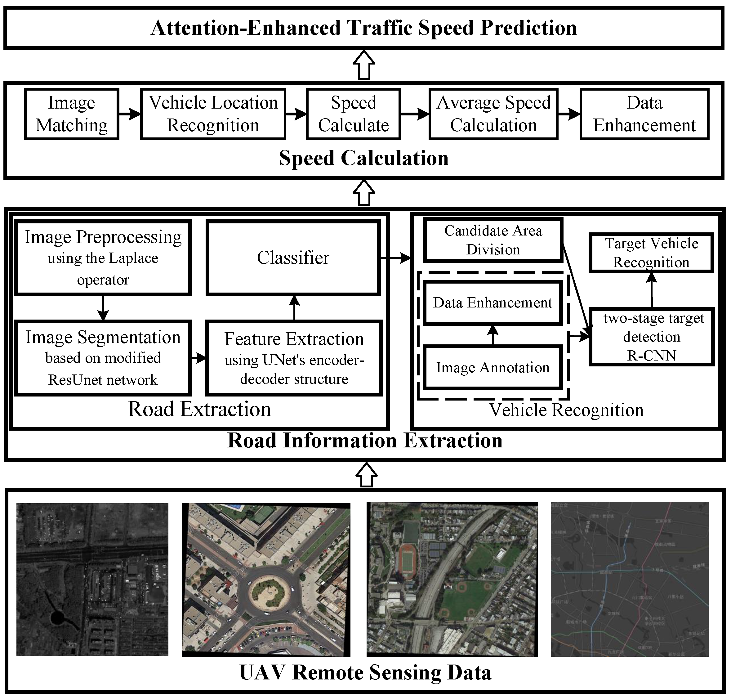
UAV imagery is usually large in scope and rich in information, containing other scenes such as buildings and roads. We aim to obtain traffic information from UAV imagery, so extracting road areas is a key point.

Firstly, the UAV imagery is pre-processed. During the formation and transmission of UAV imagery, the weather, light, system noise, and shadows of features may influence the image quality. We use the Laplace operator to sharpen the images and highlight the detailed features of the images. Secondly, we use a modified ResUnet network to extract features from the images, using UNet’s encoder–decoder structure to capture more contextual information and improve the accuracy and efficiency of the road area extraction.

4.2. Vehicle Identification

We use the R-CNN two-stage target detection algorithm to identify vehicles in the UAV imagery. Candidate regions are first generated using image segmentation, and each region is scaled to a uniform size to extract features. Regions with similar features, such as color and texture, are combined with filtering out possible vehicle locations. Then, the candidate regions are fed into a convolutional neural network for spatial feature extraction. Finally, the extracted features are fed into an SVM for sample classification to identify the vehicle. The two-stage target detection algorithm can identify objects in the figure more accurately and detect the location of the objects.

4.3. Vehicle Speed Calculation

By combining panchromatic and multispectral images, we can estimate the vehicle speed by calculating the vehicle’s displacement. Due to the different sensor positions, there is a small time difference between the panchromatic and multispectral images. The vehicle position cannot be extracted directly from the multispectral image due to the low resolution of the multispectral image. Therefore, based on the vehicle position extracted in the high-resolution image, the panchromatic image is matched with the multispectral image to indirectly obtain the vehicle position in the multispectral image, which calculates the vehicle displacement and then estimates the vehicle speed based on the difference in imaging time between the two. The steps are first to use the principal component analysis method to perform multi-band multispectral image conversion to obtain a multispectral image. Secondly, the panchromatic and multispectral images are adjusted to the same resolution to obtain the vehicle template and the target image. Finally, the position of the target vehicle in the multispectral image is obtained by the similarity matrix calculation.

As there is a limit to the speed at which vehicles can travel in the road area, the vehicle displacement is not large for a short period and is reflected in the image by about 20–30 pixels. The size of the vehicle template in the panchromatic image is N × M, and the size of the target image is N${}^{\prime }$× M${}^{\prime }$, and then its length and width correspond to

$$N^{\prime }=N+\frac{2v\Delta t}{p},$$

(1)

$$M^{\prime }=M+\frac{2v\Delta t}{p},$$

(2)

where v is the maximum vehicle speed, $\Delta t$ is the imaging time difference between the multispectral and panchromatic images, and p is the image resolution.

In the panchromatic and multispectral image stages, the vehicle template is matched for similarity with each possible position of the vehicle in the target image to obtain a similarity matrix, the value of which corresponds to the degree of matching at this position, and the maximum value in the similarity matrix indicates the position of the vehicle template in the target image. We use the spatial cosine theorem to calculate the similarity between the vehicle template and the target image:

$$p_{ij}=\frac{{\sum }_{m=1}{\sum }_{n=1}\left(A_{m,n}\times B_{i+m,j+m}\right)}{\sqrt{{\sum }_{m=1}{\sum }_{n=1}{A}_{m,n}^2}\sqrt{{\sum }_{m=1}{\sum }_{n=1}{B}_{i+m,j+n}^2}},$$

(3)

where A is the vehicle template, B is the target image, and i and j denote the position in the target image. By selecting the maximum value of the similarity matrix, the vehicle’s position in the multispectral image can be located to calculate the vehicle’s displacement at different time phases, and the vehicle speed information can be estimated.

The average speed of a road is an important parameter of traffic state in this paper, which can better reflect the operation state of traffic in a specific section and time period. The calculation method is shown in Equation (4). We select the average speed of the road $v_l$ as the characteristic parameter of traffic state for analysis and prediction:

$$v_l=\frac{1}{N}\sum _{i=1}^N{v}_i.$$

(4)

4.4. GPS Data Enhancement

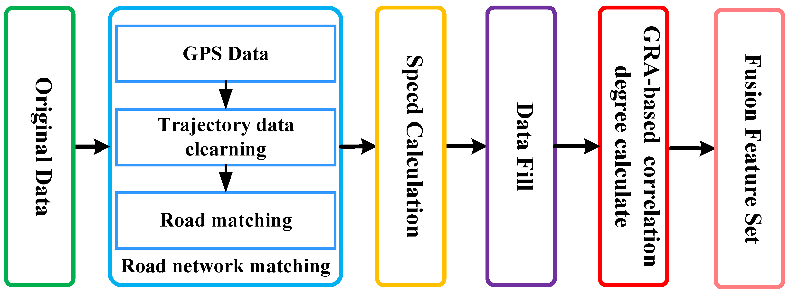
UAV remote sensing data are periodic and sparse, which has a certain impact on the accuracy of the prediction. Given that the data may be lost or abnormal in the process of data collection and transmission, the GPS data are initially preprocessed, and feature extraction is then performed. The process of trajectory data preprocessing and feature extraction is shown in Figure 3.

In this paper, we take the Chengdu taxi trajectory data as original data that include the road name, road number, the longitude and latitude of the starting point of the road, and the length of the road. The final data of the traffic characteristic parameters are obtained by cleaning the original GPS data, matching road, calculating average speed, processing abnormal and missing value, fusing external feature data, and extracting spatial feature.

We select the target road network data from the original data. The target road network consists of nodes and roads; long roads are divided into short roads based on the traffic lights. We match the selected trajectory data with roads by the longitude and latitude range of the start point and end point of the road, completing the road network matching.

We calculate the average speed of the matched roads and complete the preliminary traffic state feature extraction based on GPS data. We set the observation period as 5 min, and extract 288 sets of traffic state features for each road section in one day. According to Equation (4) and the trajectory dataset, the average speed of each vehicle passing through the target roads in the observation period is calculated. The set of vehicles that pass through road i is denoted as $C=\{C_{i,1},C_{i,2},\cdots ,C_{i,N}\},(i=1,2,\cdots ,S)$, S is the number of roads, and the position latitude and longitude of vehicle $C_{i,k}$ at time t are denoted as $(W_{i,k,t},J_{i,k,t}),(k=1,2,\cdots ,N)$. According to the shortest spherical distance [38], the distance (unit: km) traveled by the vehicle $C_{i,k}$ from time $t-1$ to time t can be calculated as follows:

$$d_{i,k,t}=2R\times arcsin(\sqrt{{sin}^2(\frac{w_{i,k,t}-w_{i,k,t-1}}{2})}+cos{w}_{i,k,t}\times cos{w}_{i,k,t-1}\times {sin}^2(\frac{j_{i,k,t}-j_{i,k,t-1}}{2})),$$

(5)

where R is the radius of the earth.

The average speed (unit: km/h) of the vehicle $C_{i,k}$ in the t-th time interval is defined and calculated by

$${\overline{v}}_{i,k,t}=d_{i,k,t}÷(\frac{5}{60}).$$

(6)

The average speed of N vehicles on road section i in the t-th time interval is calculated to obtain the average speed $v_{i,t}$ (unit: km/h) of the road section in the t-th time interval, shown as follows:

$$V_{i,t}=\frac{1}{N}\sum _{k=1}^N{\overline{v}}_{i,k,t}.$$

(7)

The missing data are mainly for the period of less traffic flow, which may lead to the missing average speed data due to no vehicles passing through during the observation time. The average speed threshold in this paper is set as

$$0<V_{i,t}\le {\varphi }_V{V}_f,$$

(8)

where $V_f$ is the limited speed specified in the observation section, ${\varphi }_V$ is the correction factor, and the range usually takes [1.3, 1.5].

For the missing and abnormal data, we use a time-series average method to interpolate such values. The time-series average method takes the current time data as the center and takes the arithmetic average value of the average speed of several adjacent periods in the current time period as the traffic state characteristics at the current time, calculated by Equation (9):

$${\widehat{V}}_{i,t}=\frac{1}{2n}(V_{i,t-n}+V_{i,t-1}+V_{i,t+1}+V_{i,t+n}+3L).$$

(9)

In Equation (9), ${\widehat{V}}_{i,t}$ is the estimated value of the average speed of the road with a missing or abnormal interval in the t-th format interval, and $2n$ is the group number of adjacent periods. This method is suitable for those with fewer missing values. To meet the real-time requirements of traffic forecast and the demand of intelligent traffic guidance, n should not be too large here, usually $n=1$.

When the data of a certain period of time are continuously missing, the later experimental error will be relatively large by using the time-series average method to fill the data. Therefore, we use the least squares polynomial fitting method to fill the data, calculated by Equation (10):

$$f\left(v\right)=a_0+a_{1}v+a_2{v}^2+\cdots +a_{n-1}{v}^{n-1}+a_n{v}^n.$$

(10)

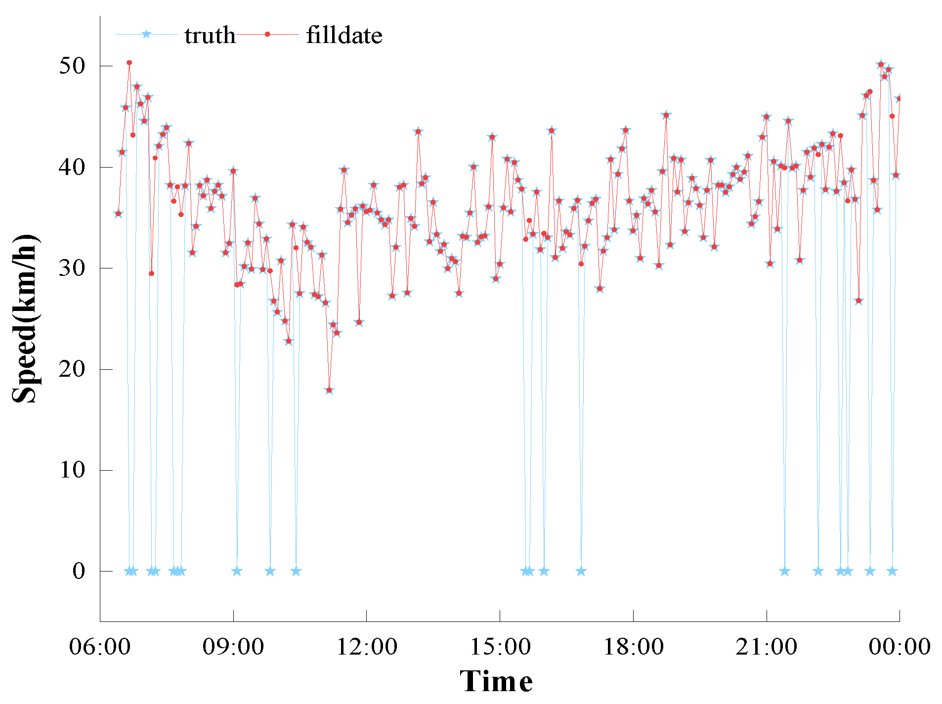
On the basis of the above analysis, we process the track data of vehicles to obtain the final set of traffic characteristic parameters. The trajectory data of vehicles are extracted for preprocessing and traffic state feature extraction, which travel from north to south in 1 to 2 November 2016 at Julidi Middel Road. A total of 576 groups of characteristic parameters are obtained, as shown in Figure 4. From the figure, the average speed of the road section, which is a characteristic parameter of traffic state, can express the traffic operation trend and state after preprocessing the original track data. By processing the missing and abnormal data, the curve of the average speed of the road section becomes complete and smooth.

4.5. Data Correlation Analysis Based on GRA

Traffic prediction can not only provide a scientific basis for traffic managers, perceive traffic congestion in advance, and restrict vehicle driving but also provide a safe road choice and guarantee the improvement of travel efficiency for urban passengers. However, traffic forecasting has always been an arduous task due to its complex spatiotemporal dependence.

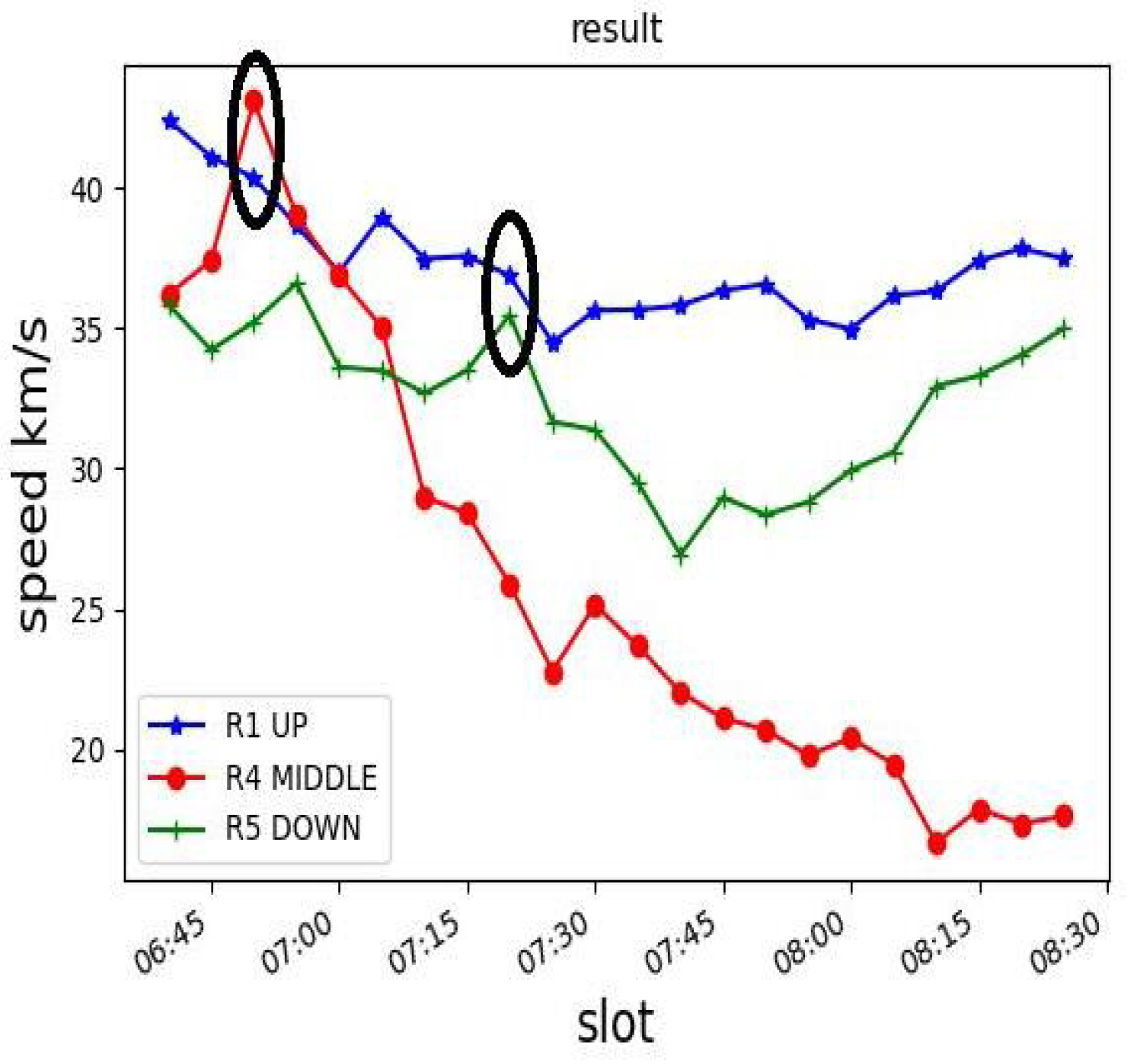
It is well known that traffic data have strong spatiotemporal correlation with each other, which poses a challenge for traffic speed prediction. The spatial change of traffic speed is mainly determined by the topological structure of an urban road network. The traffic condition of the upstream road affects the traffic condition of the downstream road through the transmission effect, and the traffic condition of the downstream road affects the traffic condition of the upstream through the feedback effect. 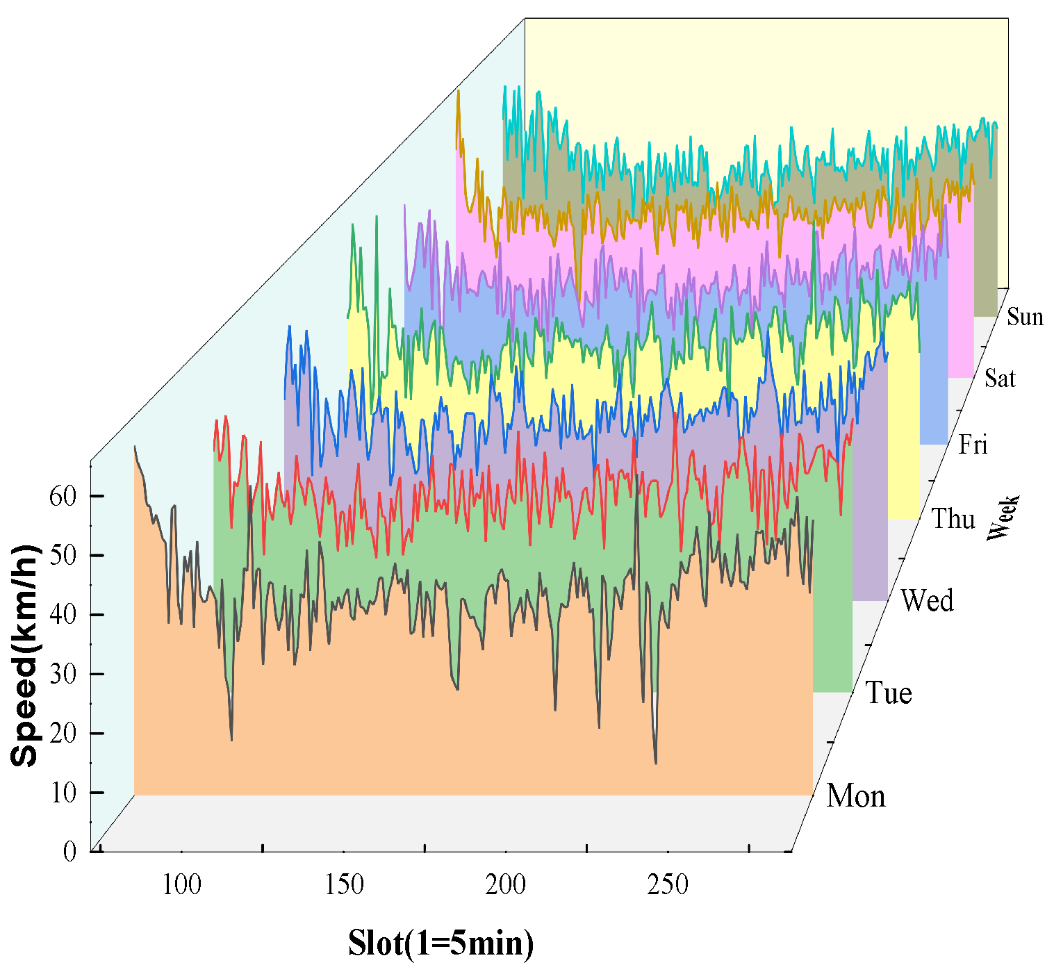As shown in Figure 5, the average speed of a certain road section is not only affected by the historical traffic state of a single section but is also closely related to the traffic conditions of adjacent sections. The dynamic change of the road speed with time is mainly reflected in the periodicity and trend. As shown in Figure 6, the traffic speed on road 1 shows a similar daily variation trend from Monday to Sunday.

We use GRA to solve the complex spatiotemporal dependence problem. GRA examines the correlation degree of various factors in a system by comparing the similarity between the geometric shapes of each factor curve [39]. It has the advantages of a small amount of data, convenient calculation, and no need to calculate statistical characteristics, and its analysis results are basically consistent with the results of qualitative analysis. To find the adjacent roads that are related to the traffic speed of the target section, this paper chooses to use the gray correlation analysis to measure the correlation degree between the adjacent sections in the peak period.

Assuming that the target road has l adjacent roads, we determine the influence degree of adjacent roads on the target road by using GRA. We use $v_0\left(t\right)$ to denote the traffic state feature sequence of the target road $v_i\left(t\right)(i=1,2,\cdots ,l)$ to denote the traffic state feature sequence of adjacent roads. The computation steps are as follows.

Step 1: The difference between the target road sequence and the adjacent road sequence at each time point is calculated by

$${\Delta }_i\left(t\right)=|v_0\left(t\right)-v_i\left(t\right)|,$$

(11)

and

$${\Delta }_i=({\Delta }_i\left(1\right),{\Delta }_i\left(2\right),K,{\Delta }_i\left(l\right)),$$

(12)

where n is the length of the sequence, $t=1,2,\cdots ,n$.

Step 2: Equation (13) calculates the gray correlation coefficient ${\gamma }_i\left(t\right)$ between the target link sequence $v_0\left(t\right)$ and the adjacent link sequence $v_i\left(t\right)$ at each time point. The correlation coefficient reflects the closeness of the two compared sequences at each time point $0<\gamma \le 1$:

$${\gamma }_i\left(t\right)=\frac{{\Delta }_{i}min+{\Delta }_{i}max}{v_i\left(t\right)+{\Delta }_{i}max},$$

(13)

where ${\Delta }_{i}max$ and ${\Delta }_{i}min$ are the maximum and minimum differences between the feature sequence of road i and the feature sequence of the target road section, respectively.

Step 3: Equation (14) calculates the gray correlation degree between the traffic state characteristics of the target road section and the adjacent road section:

$${\gamma }_{0,i}=\frac{1}{n}\sum _{i=1}^n{\gamma }_i\left(t\right).$$

(14)

The gray correlation degree of each road section in the neighboring area is sorted with the target road section. The greater the correlation degree, the greater the influence of the adjacent section on the traffic state of the target section, which can be used as the basis for extracting the spatial characteristics of traffic speed.

5. Vehicle Speed Prediction Based on Deep Learning

5.1. LSTM Network

The LSTM network is a special type of recurrent neural network (RNN). It can learn long-term dependent information and overcome the shortcomings of traditional RNN. In the dynamic gate structure of LSTM, the forgetting gate controls whether the current moment memory module retains the hidden cell state of the upper layer with a certain probability, which reads as $h_{t-1}$, $x_t$ and $C_{t-1}$. $h_t$ is the output of time t of the LSTM memory unit, and C is the state of the memory unit. $f_t$ outputs a value between 0 and 1, with 0 for complete discard and 1 for full reservation.

Usually, when using LSTM to perform natural language processing, a softmax layer is added at the end of the LSTM layer as the final output. The traffic speed prediction in this paper belongs to a regression problem. Therefore, we add the linear transformation layer after LSTM as the final predicted value output and use the gradient descent method to train the model. Moreover, the objective function in the training process is the sum of mean square errors (MSEs) between the predicted and actual values.

To minimize the training error, the Adam algorithm is used as the optimization algorithm, which is an adaptive learning rate algorithm. Adam calculates the first and second moments of each parameter according to the loss function. The learning rate of each parameter is dynamically adjusted to make the parameter change stable during the training process. The convergence speed of Adam is fast, and the learning effect in the training process is good. In addition, the dropout mechanism [40] is introduced into the network to prevent the model from overfitting. The input nodes and recursive connections are inactivated with a certain probability during the training process, which reduces the interaction between nodes and strengthens the generalization ability of the model.

5.2. Principle of Attention Mechanism

Although LSTM introduces a memory unit to determine the information to be retained or removed through its “gate” structure, obtaining the final reasonable vector representation with a long time series is still difficult. In addition, when the time span is large, the calculation will be heavy and the time consumption will be extremely long.

The attention mechanism is a method for solving problems by imitating human attention. It can quickly screen high-value information from a large number of information, which is mainly used to overcome the limitations of the LSTM feature extraction. The attention mechanism selectively learns these inputs when it trains a model, and associates the output sequence when it outputs a model, which achieves information filtering.

In our model, we combine an attention mechanism with gated convolution to adaptively adjust the key features importance, where the importance of value can be calculated as

$$E=V_e·\sigma (ReLU(X·a)+b_e),$$

(15)

and

$$E_{i,j}^{{}^{\prime }}=\frac{exp\left(E_{i,j}\right)}{{\sum }_{i=1}^{T_{r-1}}exp\left(E_{i,j}\right)},$$

(16)

where $a=softmax\left(X\right)$, $V_e$ and $b_e$ are learnable parameters, E is the correlation matrix, $E_{i,j}$ is the strength of dependence between i and j, and $E_{i,j}^{{}^{\prime }}$ is the attention value.

5.3. ATLSTM Model Construction

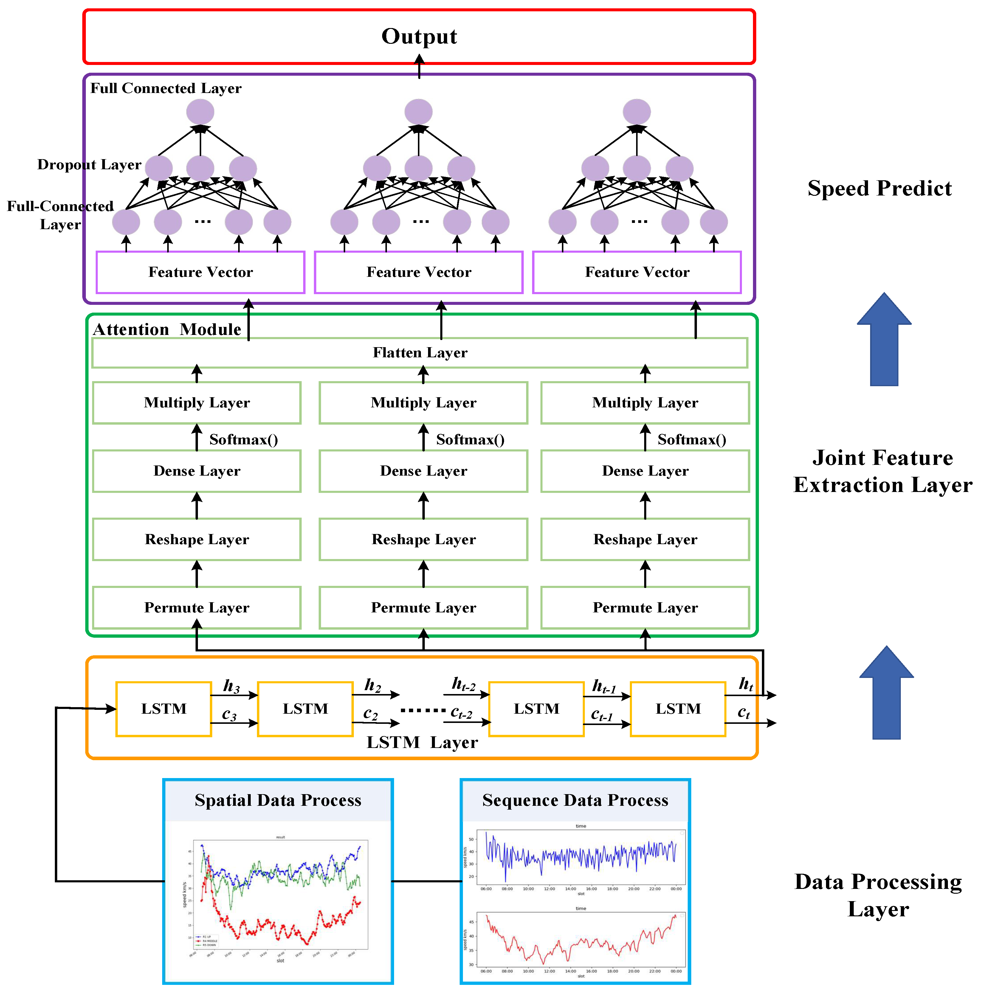
In view of the spatial dynamic instability and long-term time dependence of the road traffic speed, we introduce the attention mechanism into LSTM. By combining the unique unit structure of LSTM and attention in mining temporal and spatial series data rules, ATLSTM weighs all of the input features one by one, pays attention to the specific space and channel, extracts significant fine-grained feature information of the space–time series, and then predict the traffic speed. The structure of the model is shown in Figure 7.

We aim to predict the average speed of the target section in the $t+1$ time interval according to the historical traffic speed of the target road in $[t-p,t]$ time period and the traffic speed of the four adjacent roads of the target road. In the data preprocessing stage, the traffic data and external influence data in the historical data are initially extracted and time correlated to form the fusion feature set. Then, through the GRA, the data of four adjacent roads are extracted to form the final feature set, which are more closely related to the target road space.

In the stage of traffic speed prediction, the training set data are initially inputted into the LSTM network for training. The LSTM network trains the set data and then extracts the characteristics of short-term time series. The data trained by the LSTM network are inputted into the attention mechanism, which consists of five layers, i.e., permute, reshape, dense, permute and multiply layers. The first permute layer converts the received LSTM data into a specific format. The reshape layer transforms the data into a specific shape. The dense layer activation function selects softmax to calculate the weight of each feature, which is the density layer in the attention structure. In this paper, the attention weight of multi-dimensional features in attention is not shared.

Given that the second structure of attention is multiplication, it needs to multiply the corresponding elements. Thus, the second permute layer is used to transform the dimension again. In the multiply layer, the weight is multiplied by the input, and the attention layer is finished. After the flatten layer, the multi-dimensional data are tiled into one dimension and connected with the output layer. Finally, through the full link layer, the average speed of after 5 min is predicted.

6. Experiment Analysis

6.1. Experiment Settings

In this section, the Jiulidi Middle Road in Chengdu is selected as the target section, and the coordinates range from [104.057548, 30.698718] to [104.057468, 30.696901], and the vehicle trajectory data [41] from north to south are collected as traffic data. The road section information is from the Chengdu Traffic Administration Bureau. The data related to the date and time, such as holidays (weekends), are generated by the actual situation.

The above data are preprocessed and feature extracted by the methods described in Section 5.1 and Section 5.2. The data from 1 to 21 November are selected as train samples, and the data from 22 to 23 November are selected as test samples. The prediction model is sensitive to the numerical range of the training input data. Thus, we use the min-max normalization method to linearly transform the traffic state characteristics and map the data to the interval [0, 1], which does not change the overall the trend of the original data. In this manner, the network can converge quickly and eliminate the influence of different data orders on the training effect of the model.

In the existing prediction model, no good method is available to determine the parameters, which are usually obtained by repeated experiments based on relevant experience. We establish a prediction model with two-layer LSTM and an attention mechanism. There is a dense layer behind the two-layer LSTM. The activation function is linear. The dropout function is used in the hidden layer of the LSTM model, and $20\%$ nodes are selected to discard each round of weight update. The loss function is MSE, and the optimization algorithm is Adam. In the attention mechanism, the softmax function calculates the weight of each feature, and the attention weight of the multi-dimensional features is not shared. Multi-attention calculates the attention value. Through the fully connected layer, the average speed of after 5 min is predicted. The six types of comparison algorithms selected in this paper are LSTM, GRU, SAEs, CNNLSTM, GCN, and TGCN.

6.2. Evaluation Metrics

We adapt five performance metrics to evaluate the effectiveness of the proposed algorithm, which are described in detail as follows.

Mean absolute error (MAE):

$$MAE=\frac{1}{n}\sum _{t=1}^n|y_t-{\widehat{y}}_t|,$$

(17)

where $y_t$ is the average speed of the actual road vehicle in the t time interval, ${\widehat{y}}_t$ represents the predicted value of the t time interval, and n is the number of samples.

Mean squared error (MSE):

$$MSE=\frac{1}{n}\sum _{t=1}^n{(y_t-{\widehat{y}}_t)}^2.$$

(18)

Mean absolute percentage error (MAPE):

$$MAPE=\frac{1}{n}\sum _{t=1}^n\frac{|y_t-{\widehat{y}}_t|}{y_t}.$$

(19)

Fitting degree of the model ${\mathit{R}}^{\mathbf{2}}$: When evaluating the designed prediction model and comparing the prediction results with the actual situation, the larger the fitting degree, the better the fitting degree will be. The method is defined as Equation (20):

$${\mathit{R}}^{\mathbf{2}}=\mathbf{1}-\frac{{\mathit{S}\mathit{S}}_{\mathit{r}\mathit{e}\mathit{s}\mathit{i}\mathit{d}\mathit{u}\mathit{a}\mathit{l}}}{{\mathit{S}\mathit{S}}_{\mathit{t}\mathit{o}\mathit{t}\mathit{a}\mathit{l}}}=\frac{{\sum }_{\mathit{i}=\mathbf{1}}^{\mathit{n}}{({\mathit{y}}_{\mathit{i}}-{\widehat{\mathit{y}}}_{\mathit{i}})}^{\mathbf{2}}}{{\sum }_{\mathit{i}=\mathbf{1}}^{\mathit{n}}{({\mathit{y}}_{\mathit{i}}-{\sum }_{\mathit{i}=\mathbf{1}}^{\mathit{n}}{\mathit{y}}_{\mathit{i}})}^{\mathbf{2}}}.$$

(20)

Accuracy (ACC): the accuracy of the model prediction is calculated as follows:

$$\mathit{A}\mathit{c}\mathit{c}\mathit{u}\mathit{r}\mathit{a}\mathit{c}\mathit{y}=\mathbf{1}-\sum _{\mathit{n}}^{\mathit{i}=\mathbf{1}}\frac{{\mathit{y}}_{\mathit{i}}-{\widehat{\mathit{y}}}_{\mathit{i}}}{{\mathit{y}}_{\mathit{i}}}.$$

(21)

6.3. Spatial Correlation Analysis of Traffic Data

We analyze seven roads in the 3rd North Section of the First Ring Road in Chengdu. We find that the traffic speed trends of adjacent road sections have different degrees of similarity. Therefore, when predicting the traffic speed of a certain road, it is necessary to consider the influence of the adjacent area roads.

Table 2. Correlation coefficient between road 1 and adjacent roads.

Week	Road 2	Road 3	Road 4	Road 5	Road 6	Road 7
Monday	0.798	0.819	0.786	0.735	0.722	0.840
Tuesday	0.797	0.796	0.771	0.683	0.728	0.833
Wednesday	0.790	0.819	0.824	0.708	0.695	0.808
Thursday	0.794	0.787	0.789	0.673	0.670	0.814
Friday	0.772	0.855	0.797	0.656	0.665	0.805
Saturday	0.821	0.729	0.792	0.740	0.669	0.786
Sunday	0.812	0.808	0.788	0.709	0.654	0.777
AveRelate	0.791	0.802	0.792	0.700	0.686	0.809

shows the correlation degree between each road in the selected area and target road. The correlation degree of the adjacent roads to the target road is different. The bigger the correlation degree, the greater the influence on the traffic speed of the target road will be.

When too few adjacent roads are used for the prediction, it cannot make full use of the spatial correlation of traffic speed, while too many adjacent roads may produce noise data and affect the prediction accuracy. So we select four adjacent roads, whose average correlation degree is greater than 0.7 in a week, to help predict speed. As we can see in Table 2, the adjacent road 2, road 3, road 4, and road 7 are selected to predict the target road speed.

6.4. Speed Prediction Results Analysis of GATLSTM

To reduce the input data dimension and improve the efficiency of the algorithm, for the traffic state prediction at time $\mathit{t}$, we select the first half hour, that is, the traffic speed in the time period $[\mathit{t}-\mathbf{5},\mathit{t}]$ and the speed of the four adjacent road sections with a higher degree of correlation as the traffic feature sequence input of the prediction algorithm.

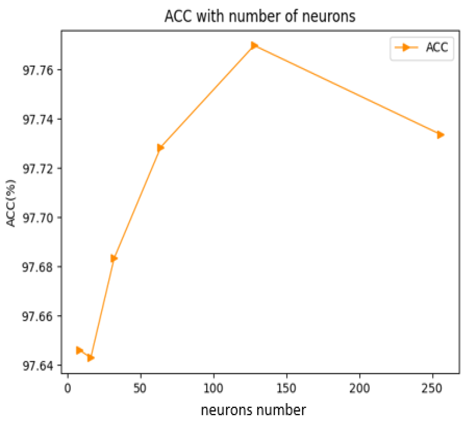
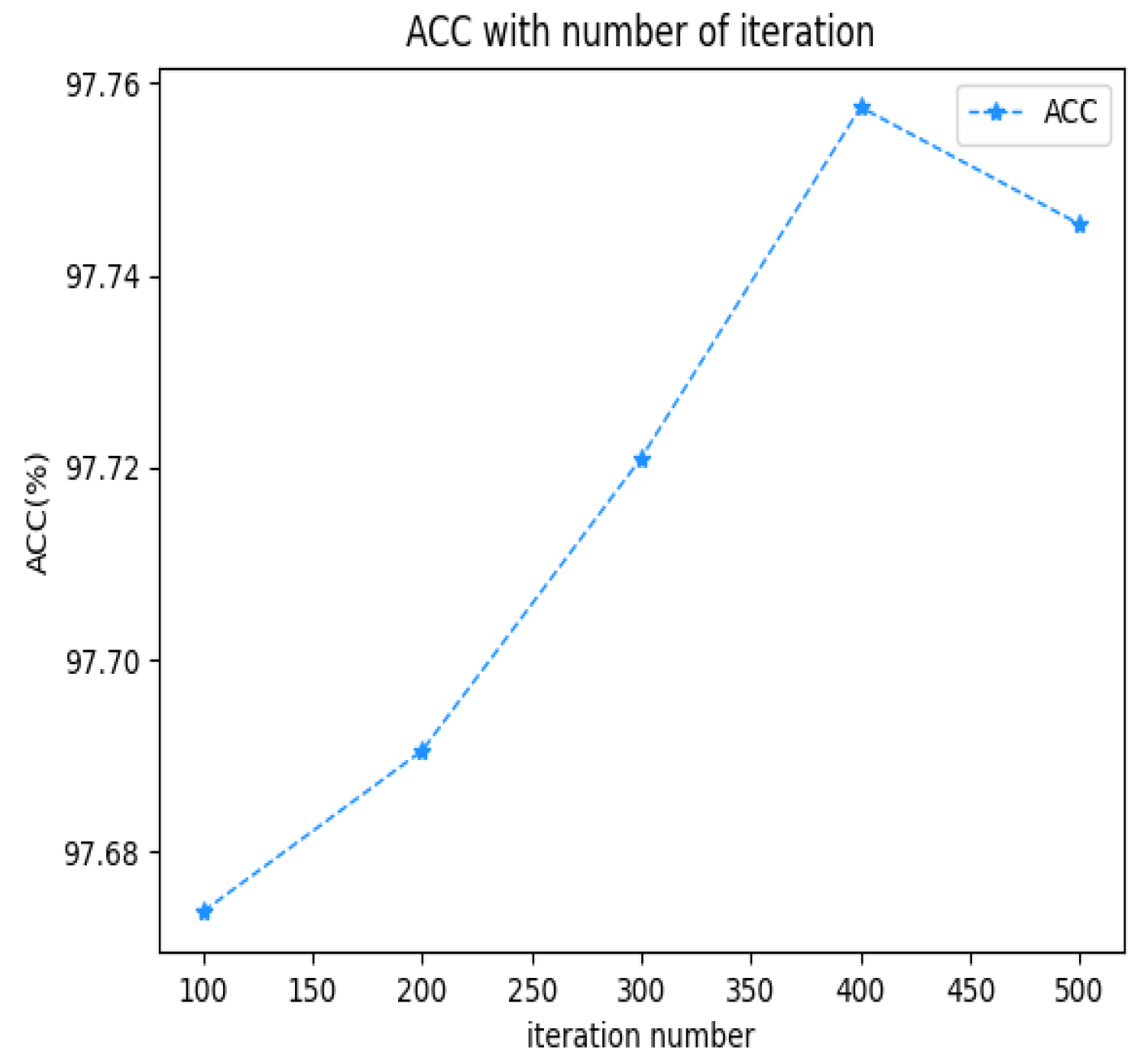
To control the complexity of the model and the accuracy of model prediction, we change the number of neurons and the number of iterations in conducting the experiments. As shown in Figure 8, the prediction accuracy of the model increases with the number of neurons. When the number of neurons reaches 128, the prediction accuracy of the algorithm decreases instead. Thus, we select 128 as the number of neurons in each layer. As shown in Figure 9, the prediction accuracy of the model and the time for model training increases with the number of iterations. To balance the prediction accuracy and computational efficiency, we set the number of iterations as 400.

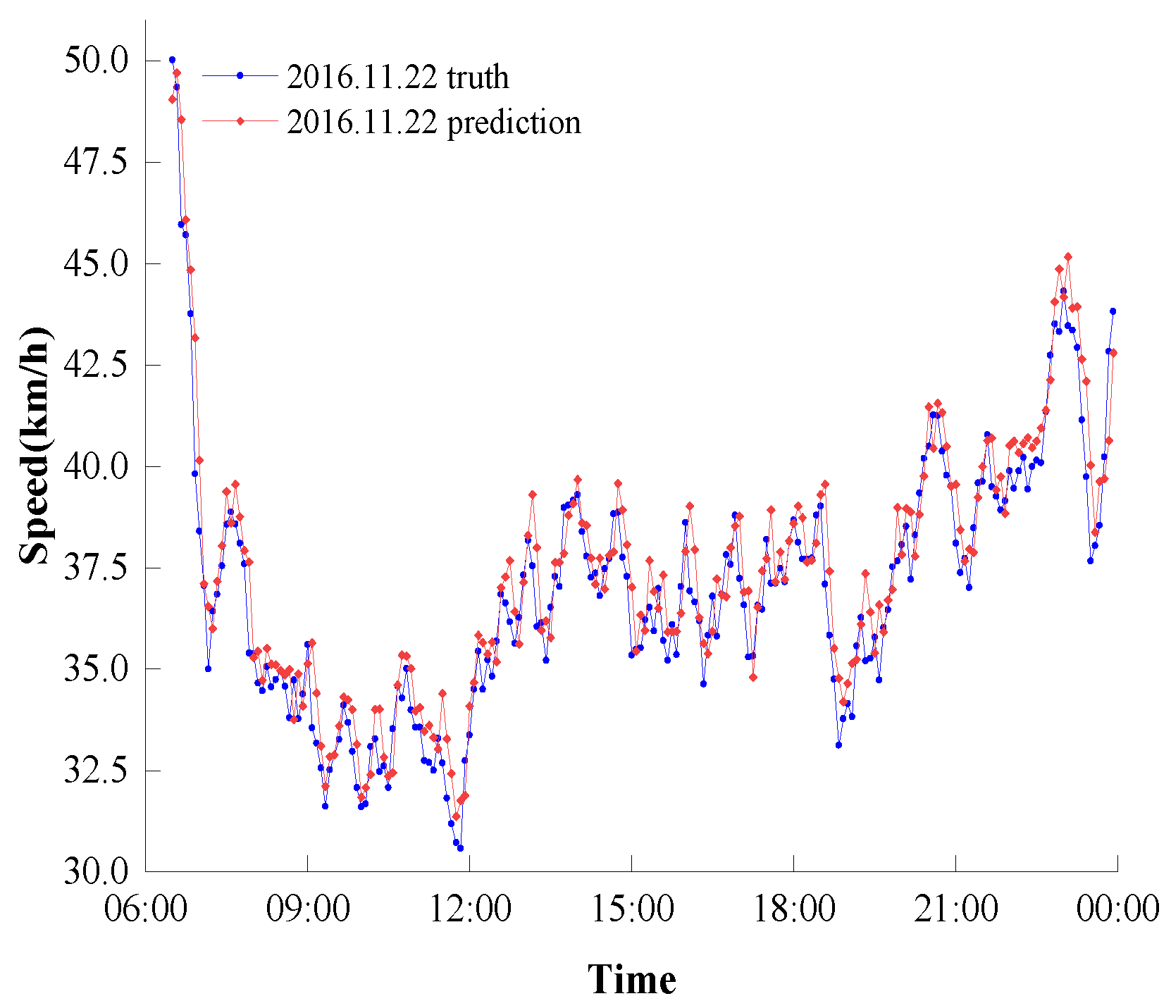
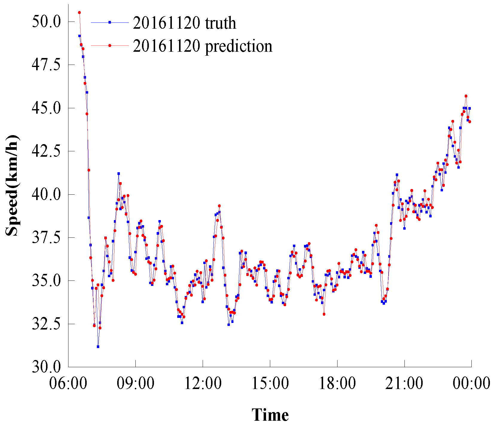
After the experimental parameters are determined, we predict the traffic speed of the target road section on weekdays and holidays (weekends). Figure 10 and Figure 11 show the prediction results of the GATLSTM. As shown from the figures, the morning rush hour is more obvious on workdays, the traffic speed fluctuates greatly throughout the day during holidays (weekends), and the evening rush hour is longer. Moreover, the traffic speed prediction curve in this paper can better fit the measured speed curve in both cases.

6.5. Comparative Experiments

To validate the effectiveness of the GATLSTM algorithm, selecting LSTM, GRU, SAEs, CNNLSTM, GCN, and TGCN models as baseline methods, we compare the proposed method with the baseline method on a real dataset.

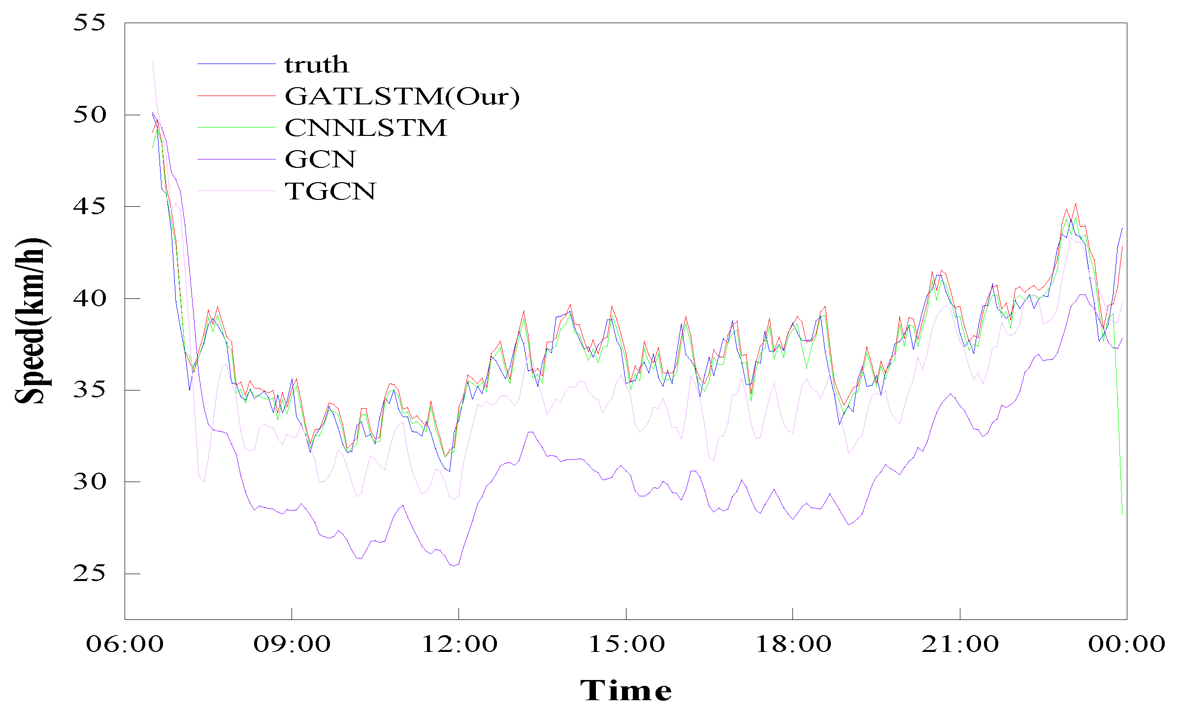
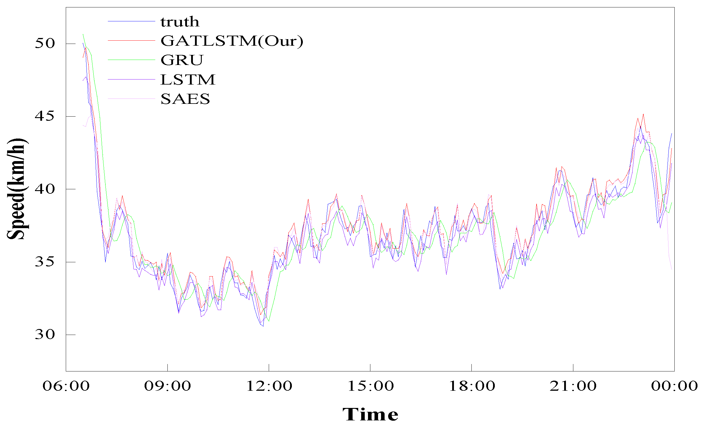
Figure 12 and Figure 13 show the results of different methods, and

Table 3. Performance measurement.

Algorithm	ACC	MAE	MAPE	RMSE	${\mathit{R}}^2$
GATLSTM	0.979	0.565	2.08	0.768	0.944
CNNLSTM	0.965	0.708	2.20	0.889	0.928
GCN	0.777	5.507	16.24	6.767	0.627
TGCN	0.866	3.052	6.48	4.076	0.865
LSTM	0.967	0.969	2.14	1.209	0.925
GRU	0.913	1.407	3.55	2.647	0.943
SAES	0.962	0.858	2.68	1.408	0.809

shows the performance metrics of different methods. In Figure 12 and Figure 13, the blue line is the real speed value of the target section, the red line is the speed value predicted by the GATLSTM model, and the other color lines are the predicted values from the baseline algorithm. The closer the distance to the blue line, the closer the prediction result is to the true value, and we can easily see that our prediction result is closest to the blue line, indicating that our proposed model can better learn the potential features between the traffic speed spatiotemporal sequences. As shown in Table 3, the MAE of the ATLSTM is the smallest, and its accuracy is the highest. Therefore, GATLSTM has the best performance compared to the baseline algorithm for this prediction problem. We also found that the prediction results of GCN and TGCN models are less accurate, which indicates that the traffic data are highly spatiotemporal correlated and the best prediction results cannot be obtained by time-series models and spatial-prediction models alone. Moreover, we conclude that GCN and TGCN may be more suitable for large cities with a complex road network, but GATLSTM is more suitable for small- and medium-sized cities. We further find that the prediction is accurate and efficient when the data pre-processing process is simple.

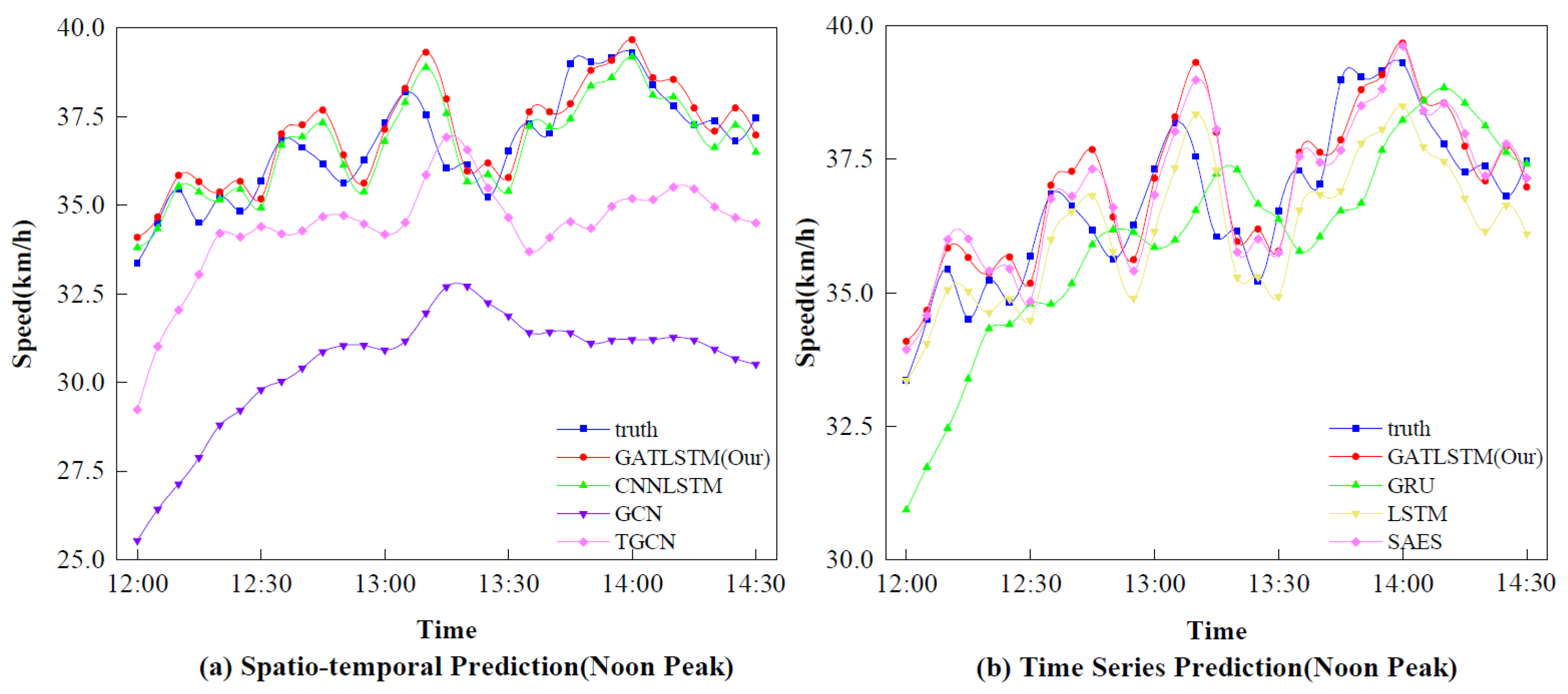
Finally, to compare the prediction effects of the models more intuitively, we compared the performance of each prediction model under the condition of large traffic flow fluctuation at 12:00–14:30. The results are shown in Figure 14. In comparison with other algorithms, our method still has the best prediction results during peak periods.

7. Conclusions

Considering that the existing physical sensor-based traffic data collection methods have high transmission costs, serious traffic information redundancy, large calculation volumes of spatiotemporal data processing, and sparse UAV imagery data, which make it difficult to ensure the real-time accuracy of traffic prediction, we use a novel end-to-end deep learning architecture to effectively improve the prediction accuracy. The architecture consists of a traffic information extraction module based on UAV imagery recognition and an attention-enhanced spatiotemporal prediction (ATLSTM) module. The traffic information extraction module deeply fuses the UAV imagery and GPS data to extract traffic information. ATLSTM extracts important fine-grained spatiotemporal features again to accurately predict short-term traffic speed. Finally, we evaluate the performance of the algorithm on a real-world dataset. Our method achieves the best prediction performance in terms of accuracy and stability, is more suitable for small- and medium-scale road networks, and significantly reduces graph-based computational complexity.