Article

Method of 3D Voxel Prescription Map Construction in Digital Orchard Management Based on LiDAR-RTK Boarded on a UGV

1
College of Science, China Agricultural University, Beijing 100193, China
2
Centre for Chemicals Application Technology, China Agricultural University, Beijing 100193, China
3
College of Agricultural Unmanned System, China Agricultural University, Beijing 100193, China
4
Tropics and Subtropics Group, Institute of Agricultural Engineering, University of Hohenheim, 70599 Stuttgart, Germany
*
Author to whom correspondence should be addressed.
Drones 2023, 7(4), 242; https://doi.org/10.3390/drones7040242
Submission received: 27 February 2023 / Revised: 28 March 2023 / Accepted: 28 March 2023 / Published: 30 March 2023
(This article belongs to the Special Issue Recent Advances in Crop Protection Using UAV and UGV)

Abstract

:
Precision application of pesticides based on tree canopy characteristics such as tree height is more environmentally friendly and healthier for humans. Offline prescription maps can be used to achieve precise pesticide application at low cost. To obtain a complete point cloud with detailed tree canopy information in orchards, a LiDAR-RTK fusion information acquisition system was developed on an all-terrain vehicle (ATV) with an autonomous driving system. The point cloud was transformed into a geographic coordinate system for registration, and the Random sample consensus (RANSAC) was used to segment it into ground and canopy. A 3D voxel prescription map with a unit size of 0.25 m was constructed from the tree canopy point cloud. The height of 20 trees was geometrically measured to evaluate the accuracy of the voxel prescription map. The results showed that the RMSE between tree height calculated from the LiDAR obtained point cloud and the actual measured tree height was 0.42 m, the relative RMSE (rRMSE) was 10.86%, and the mean of absolute percentage error (MAPE) was 8.16%. The developed LiDAR-RTK fusion acquisition system can generate 3D prescription maps that meet the requirements of precision pesticide application. The information acquisition system of developed LiDAR-RTK fusion could construct 3D prescription maps autonomously that match the application requirements in digital orchard management.

1. Introduction

In fruit production, the rational use of pesticides can reduce yield losses caused by pests and diseases. Wind-assisted application is often employed in orchards to improve the penetrability of pesticides [1,2]. During the wind transportation, only a part of the pesticide is intercepted by the canopy and deposited on the leaves, and the other part is lost to the ground and evaporated into the atmosphere.
During pesticide application, many parameters such as wind speed, sprayer type, droplet size, and spray volume can affect the distribution of pesticides in the canopy [3,4,5]. The wind speed and canopy characteristics can significantly influence the drift potential of small droplets [3,6,7,8]. In the gap between trees [4], droplets can be directly transported into the air by the wind due to the lack of canopy interception, resulting in significant drift losses [9]. Uniform spraying at the same application rate in canopies of different volume and leaf density, which is commonly used in pesticide application, ignores differences in the target canopy’s structure and makes pesticides underused or overused [10]. This may have exacerbated the problem of off-target loss and drift.
Therefore, an accurate three-dimensional model of the plant canopy can be constructed and applied to the application process to reduce the problem of pesticide drift. With the development of sensor technology, it has become possible to use industrial sensors to detect crop canopy for pesticide variable application. Currently, ultrasound sensor, LiDAR, and RGB camera are widely used to detect the canopy features. Ultrasound sensors could detect the volume of the plant canopy [11,12,13], and some specific models of ultrasound sensors which record the echo intensity can calculate the leaf density of the canopy [14,15]. The gradual reduction in the cost of Lidar equipment has led to the widespread use of Lidar for the precision pesticides application. Real-time decision making and execution of variable spraying based on accurate detection of tree structure by LiDAR has been successfully developed and tested in field experiments [16,17,18,19,20,21].
However, the real-time decoding of LiDAR data and the dynamic complexity of the canopy volume require high-performance computing equipment, which challenges the computational power of computers for the real-time acquisition and feature extraction of canopy point clouds. Meanwhile, real-time variable systems require sensors and an onboard high-performance computer on each sprayer, which means higher financial investment and cost management. It can reduce the cost of sensors and computers on each sprayer by sharing offline prescription maps. Through installation of RTK and a variable spray control system on each sprayer, while following a pre-generated prescription map with geographic information, multiple sprayers can execute variable spraying simultaneously by obtaining 3D canopy information in advance and generating prescription maps.
The main ways to obtain 3D information are terrestrial LiDAR or Unmanned Aerial Vehicle (UAV) photography [22,23,24,25,26,27]. Terrestrial LiDAR can capture rich details in the canopy and segment tree trunks, branches, and leaves, but mapping the structure of large orchards requires multiple scans at different locations that are stitched to create a complete point cloud of the orchard [19]. Plant height analysis using UAV photography is based on the structure from motion (SfM), which reconstructs the canopy surface using multi-view aerial imagery. However, because the images are captured from the air and the lower canopy is obscured by the upper canopy, there is usually a lack of details on the lower canopy. Compared to UAV photography and SfM technology, LiDAR has higher distance resolution and is unaffected by weather or wind. By fusing LiDAR with global navigation satellite systems (GNSS), information such as digital surface models (DSM) and canopy volume can be obtained [28,29,30]. However, DSM cannot be used directly for digital orchard management, especially variable rate pesticide application.
As shown in Figure 1, in this study regarding an acquisition system through integrating LiDAR and RTK in an all-terrain vehicle (ATV) which equipped an autonomous driving system, LiDAR-RTK fusion data were used to obtain canopy point clouds with geographic information, construct a digital orchard model, and generate a 3D occupancy voxel prescription map autonomously. The effectiveness of the algorithm was verified by evaluating the measurement error of tree height and the canopy details contained in the prescription maps of different voxel sizes. It could be a reference for low-cost multi-machine cooperative precision pesticide application. In addition, the voxel prescription map includes canopy dimensions and leaf density at different locations within the orchard, allowing for precise management actions such as estimating canopy biomass and pruning. Therefore, this study has the potential to provide valuable information for accurate orchard management. The main contributions of this study are as follows:
(1) A data acquisition system based on LiDAR-RTK fusion was proposed to achieve synchronized canopy point cloud acquisition and geographic information, which could serve as a reference for precise orchard management.
(2) The optimal prescription map was established under the voxel size of 0.1 m, 0.25 m, and 0.5 m.
(3) The accuracy of the voxel prescription map was evaluated by comparing the LiDAR-measured tree height to the true tree height.

2. Materials and Methods

The experimental orchard is located in Xiying Village, Pinggu District, Beijing (40.18°N, 116.97°E), planted with pears in 2019 date (Figure 2). The trees were pruned to a high spindle architecture with a row-to-row spacing of 4.5 m and a plant-to-plant spacing of 1.5 m, and the mean tree height was about 4 m. The seasonal growth stage was BBCH 91 (shoot growth completed; foliage still fully green) [31]. The weather was clear and windless during the experiment.

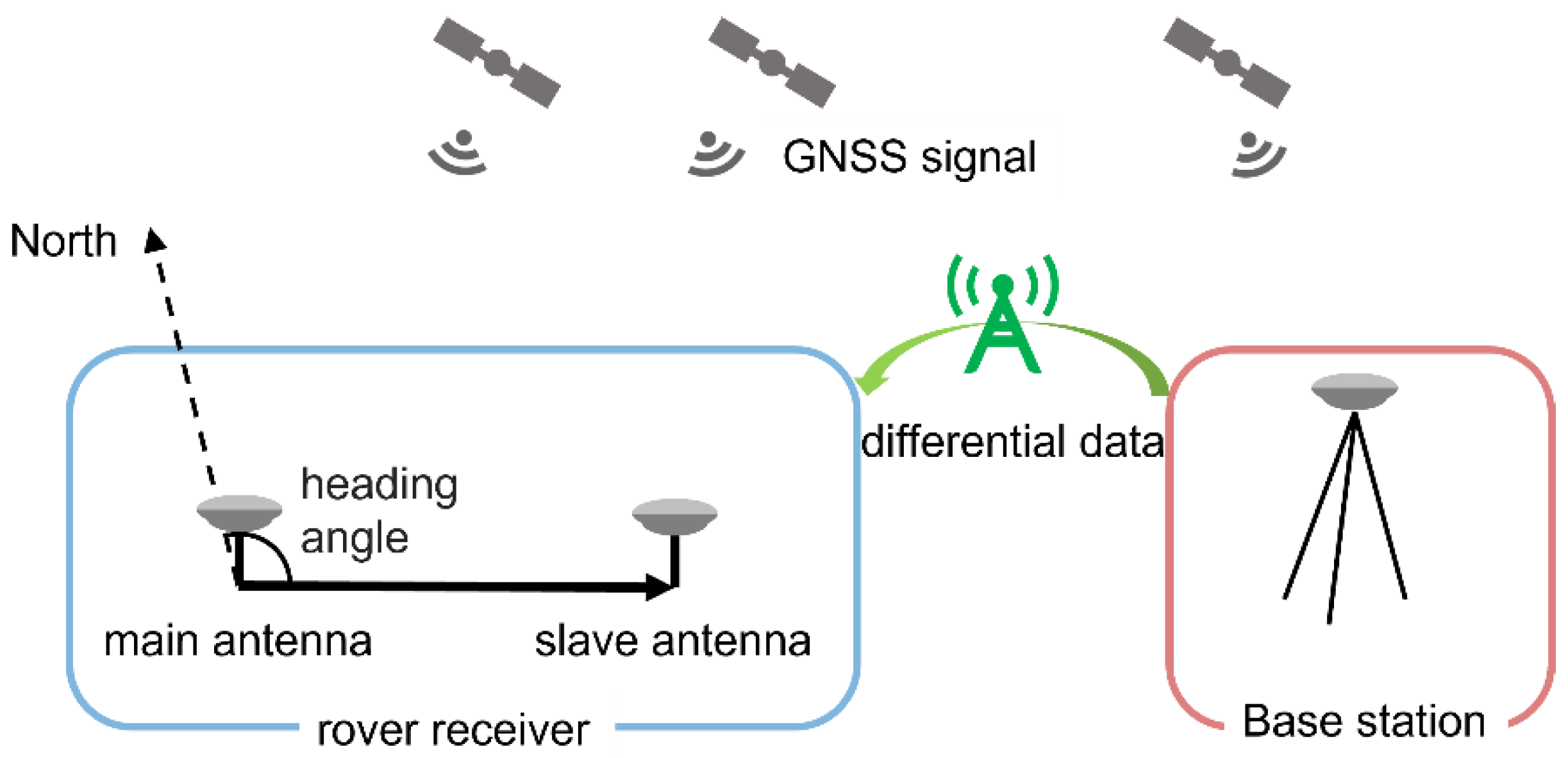
2.1. Design of the LiDAR-RTK Fusion Data Acquisition System

The hardware of the LiDAR-RTK fusion data acquisition system includes a LiDAR (RS-16, Suteng Innovation Technology Co., Ltd., Shenzhen, China), an Ethernet converter, a RTK rover with autonomous driving controller (MC5, Beijing UniStrong Science and Technology Co., Ltd., Beijing, China), an industrial computer (i7-8700T, 16G RAM, and a 1T SSD), and a battery power system (Figure 3). The Lidar was installed on an aluminum frame at 45 degrees and has 16 scan lasers, a field of vertical view of 30 degrees, a vertical resolution of 2°, a horizontal resolution of 0.1°, and a ranging accuracy of ±2 cm.
In this study, an autonomous ATV was utilized to traverse pre-determined trajectories and automatically collect digitized information from orchards. Signals from the autonomous driving controller were received by the electric steering wheel to provide precise direction control, while speed was regulated via a voltage signal.
Different installation angles of the LiDAR have a significant impact on the field of view. As shown in Figure 4a, when the LiDAR is installed vertically at 90 degrees, the scan line for downward direction is largely blocked by the ATV and only can detect the ground with weeds under the trees, which makes it difficult to split the ground. Moving the vertically mounted LiDAR forward some distance can prevent the obstruction of the ATV, but the irregular motion caused by the uneven ground may cause LiDAR to shake more. When the LIDAR is installed horizontally, its field of view is only 30°. This results in LiDAR being unable to detect the entire tree at close range, while the laser lines diverge and are widely spaced at long distance, reducing detection accuracy. Therefore, the LiDAR needs to be mounted as closely as possible to the fixation point to be able to detect the entire tree at close range.
Therefore, as shown in Figure 4b, the LiDAR was fixed at 45 degrees in this study. Given the slow forward speed and the LiDAR scan speed being set at 600 rpm, the motion distortion caused by the LiDAR rotation could be ignored.
The point cloud obtained by the LiDAR was referenced to the origin of the LiDAR. However, the prescription map used for variable application must include geographic information, the sprayer then makes control decisions based on the location, and the prescription map.
GNSS could provide the position of the antenna phase center in the geodetic coordinate system. RTK is a commonly used method to improve positioning accuracy. As shown in Figure 5, the RTK system consists of a base station and a rover station, which communicate with each other via 4G network for differential data transmission. The RTK rover station with directional function has two antennas, which could not only solve the real-time position of the main antenna but also obtain the angle between the vector from the main antenna to the slave antenna and the north direction, also known as the heading angle.
In this study, custom Python (3.8.10, Python Software Foundation) scripts were used to collect binary data from the LiDAR and RTK systems. The LiDAR point cloud data were transmitted via UDP protocol over the Ethernet in a binary format. The main data stream was sent through UDP datagrams on port 6699 by default. The RTK position statements were transmitted to the computer via a serial port at a baud rate of 115,200, and the data acquisition script stored the binary data from the LiDAR along with the position information in one file.

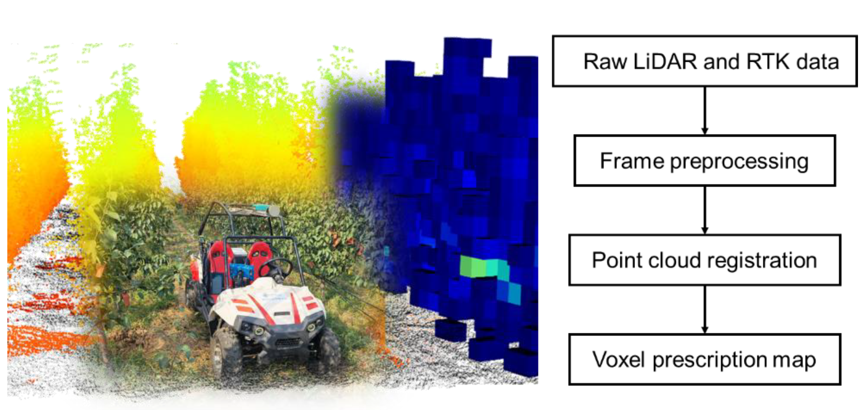
2.2. Voxel Prescription Map Generation

2.2.1. Establish the Coordinate System

The geographic coordinate system of the LiDAR-RTK fusion data acquisition system does not match the coordinate systems of the LiDAR and RTK in the initial state (Figure 6). The right-handed coordinate system was used throughout the decoding process. To reduce the additional computation and error caused by rotation of voxels, an appropriate global coordinate system was established to make the edges of the voxel parallel to the operation trajectory.
First, one point was selected as the global origin to create an East–North–Up (ENU) coordinate system, which was rotated around the z-axis until the y-axis was parallel to the tree row direction. The rotated coordinate system was used as the global coordinate system, and the rotation angle was the tree row angle. During the scanning, the ATV was driven in the middle of the tree rows, where its direction was parallel to the row of trees. Therefore, the distribution histogram can be created by analyzing the angles between the heading and the north in the travel trajectory, and the tree row angle was calculated based on its peak.

2.2.2. Point Cloud Pre-Processing

For a better stitching result, the point cloud was pre-processed in the LiDAR coordinate system. Due to the diffusion of LiDAR laser lines, fewer feature points could be detected at longer distances, while too-close noise points should also be excluded, and, finally, only points in the range of 0.2–20 m were retained.
Random sample consensus (RANSAC) is a planar segmentation method which fits randomly sampled points to a plane through multiple iterations. In this study, the plane fitting function in Open3D was directly called. The parameters were empirically set to 50 sampling points, 10,000 iterations; a distance threshold of 0.2 m. RANSAC was used to segment the ground in each frame of the LiDAR scanned point cloud. Canopy and ground points were marked differently, and only the canopy point cloud was used to construct the prescription map.

2.2.3. Point Cloud Registration

The Point cloud stitching involved multiple coordinate systems. To align all point clouds to the global coordinate system, the homogeneous coordinate was used to simplify the computations.
After decoding, the coordinate of the points was relative to the LiDAR coordinate origin. The homogeneous coordinate P l i d a r of point P in the LiDAR coordinate system is [ x , y , z , 1 ] T .
The point was rotated around the X-axis to fix the installed angle; the rotation matrix R x is Equation (1), where α is the installed angle of −45°.
R x = [ 1 0 0 0 0 c o s α s i n α 0 0 s i n α c o s α 0 0 0 0 1 ]
Then the point was transformed to the RTK coordinate system; the transform matrix T l i d a r is as follows:
T l i d a r = [ 1 0 0 t x 0 1 0 t y 0 0 1 t z 0 0 0 1 ]
where point [ t x , t y , t z , 1 ] T was the position of the LiDAR coordinate system origin in the RTK coordinate system.
The coordinate of point P in the RTK coordinate system P R T K is as follows:
P R T K = T l i d a r R x P l i d a r
The angle which was used to transform point P to the global coordinate could be calculated with Equation (4):
γ = θ h e a d i n g + θ t r e e 180
where θ h e a d i n g is the heading angle obtained by RTK rover, θ t r e e is the tree angle.
The rotation matrix R z is as follows:
R z = [ c o s γ s i n γ 0 0 s i n γ c o s γ 0 0 0 0 1 0 0 0 0 1 ]
The transform matrix T RTK which was used to move the point in the global coordinate system could be calculated using the RTK rover obtained position, so the point coordinate P g l o b a l is as follows:
P g l o b a l = T R T K R z P R T K
The point cloud in the region area was calculated by transforming all obtained points to the global coordinate system.

2.2.4. Generating Voxel Prescription Map

Digital orchard management decisions are difficult to make in real-time at a fine level based on point clouds, especially in a variable application. Therefore, a voxel prescription map must be created to extract details from the point clouds. The data were voxelized in the global coordinate system at the selected sizes, and the coordinates of the point cloud were converted to voxel indices. The number of detected points in each voxel was counted, and voxels with less than 5 points were considered as noise and ignored. Due to the acceleration and deceleration in the scan, the amount of accumulated points in the voxels varied depending on the scan time, so only the point cloud acquired under steady driving was used to generate the prescription map.

2.3. Accuracy Analysis

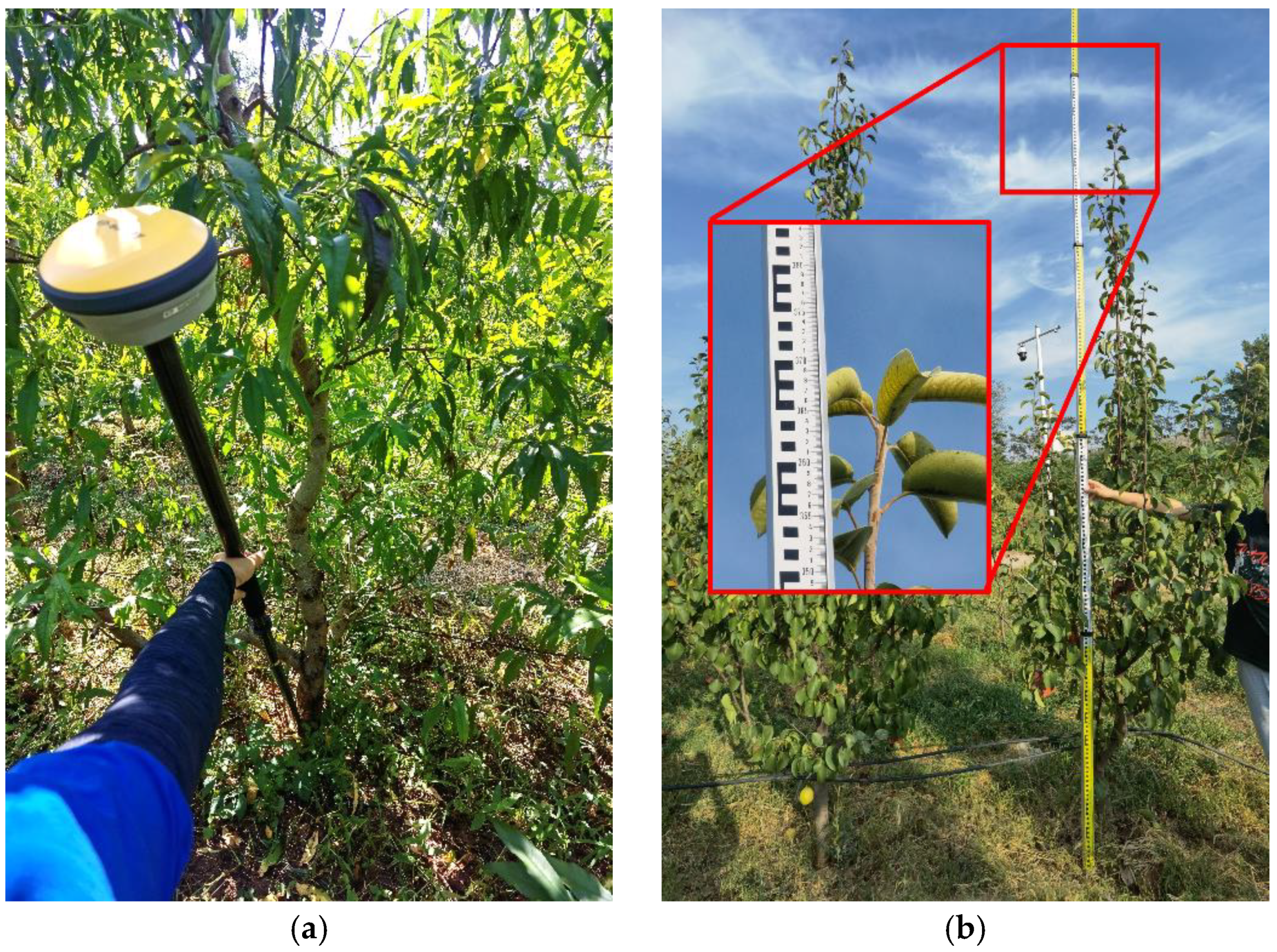
2.3.1. Ground Measurements

Tree height was defined as the distance between the tallest point of the tree and the ground. In the region area, Figure 7a, the position of the tree base were measured using a Tilt-featured RTK Receiver (E500, Beijing UniStrong Science and Technology Co., Ltd., Beijing, China), and the true height of the tree was measured using a tower ruler, Figure 7b, with a height accuracy of ±5 cm. The actual positions and true heights of 20 trees were measured.
The tree height measured by the point cloud was achieved by selecting points within 0.5 m from the root coordinates of the tree and calculating the difference between the maximum and minimum heights. The true row angles were obtained by measuring the coordinates of the trees in the six rows with a minimum of 25 tree positions measured per row and fitting them to a straight line.

2.3.2. Statistical Analysis

Root mean square error (RMSE), relative root mean square error (rRMSE), and mean absolute percentage error (MAPE) were used to evaluate the error between LiDAR measurements and true values. The equations are as follows:
R M S E = ( y i y i ) 2 n
r R M S E = R M S E y ¯ * 100 %
M A P E = 100 % n | y i y i y i |
where y i is true values, y i is predicted values, n is the total number of samples, y ¯ is the mean of n true values.

3. Results

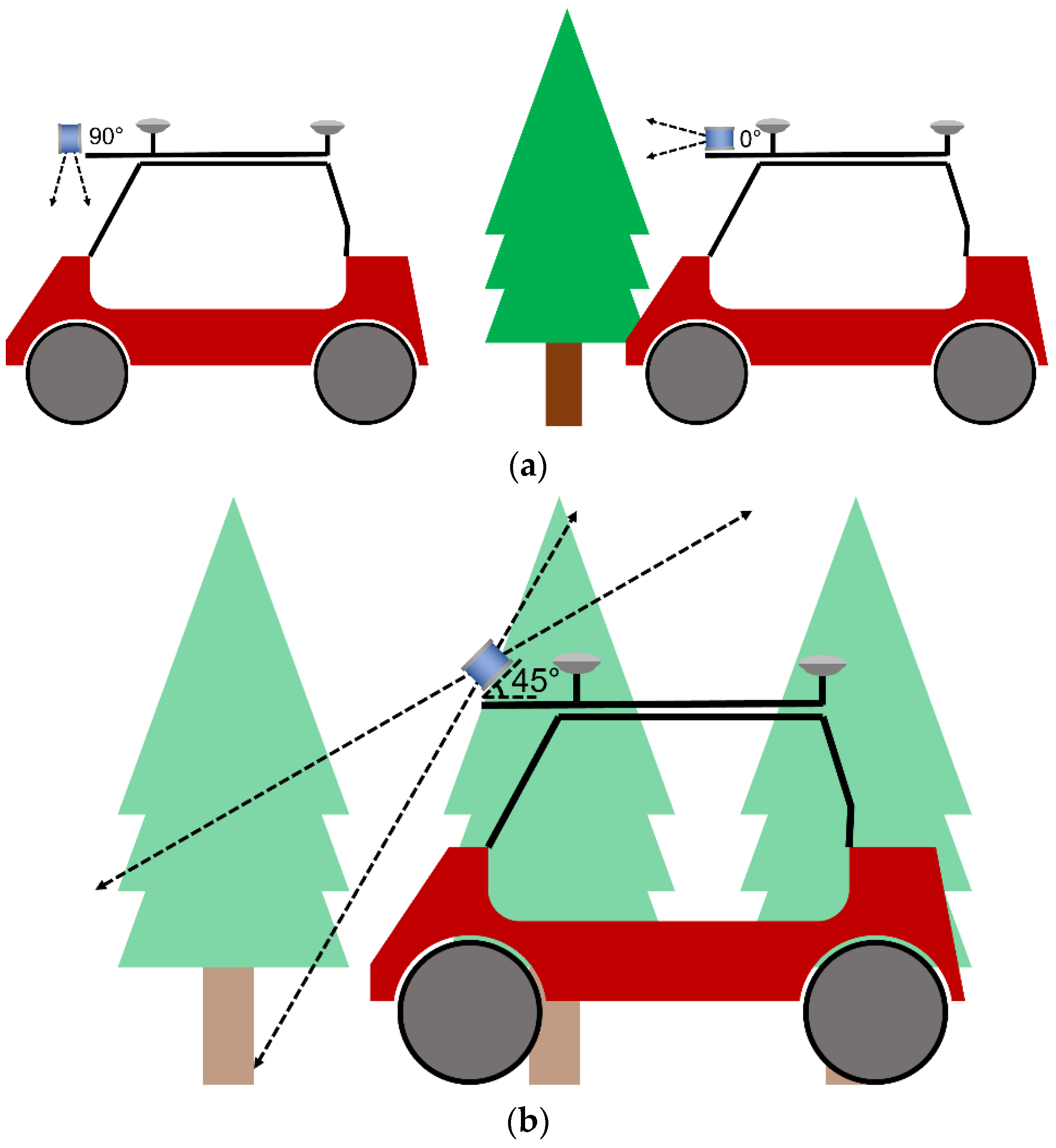
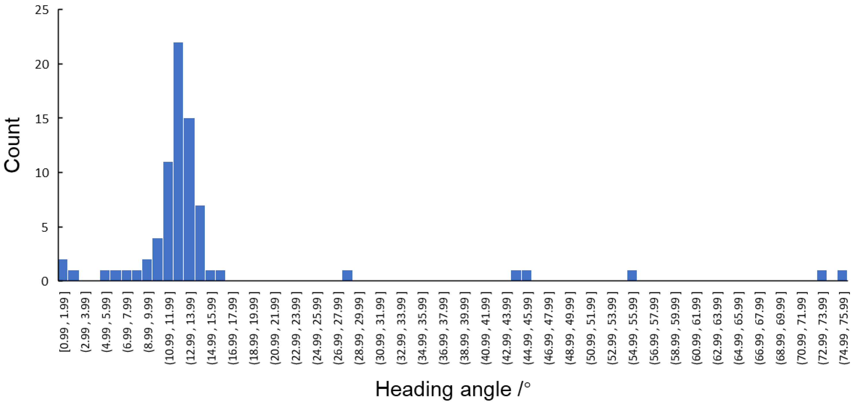
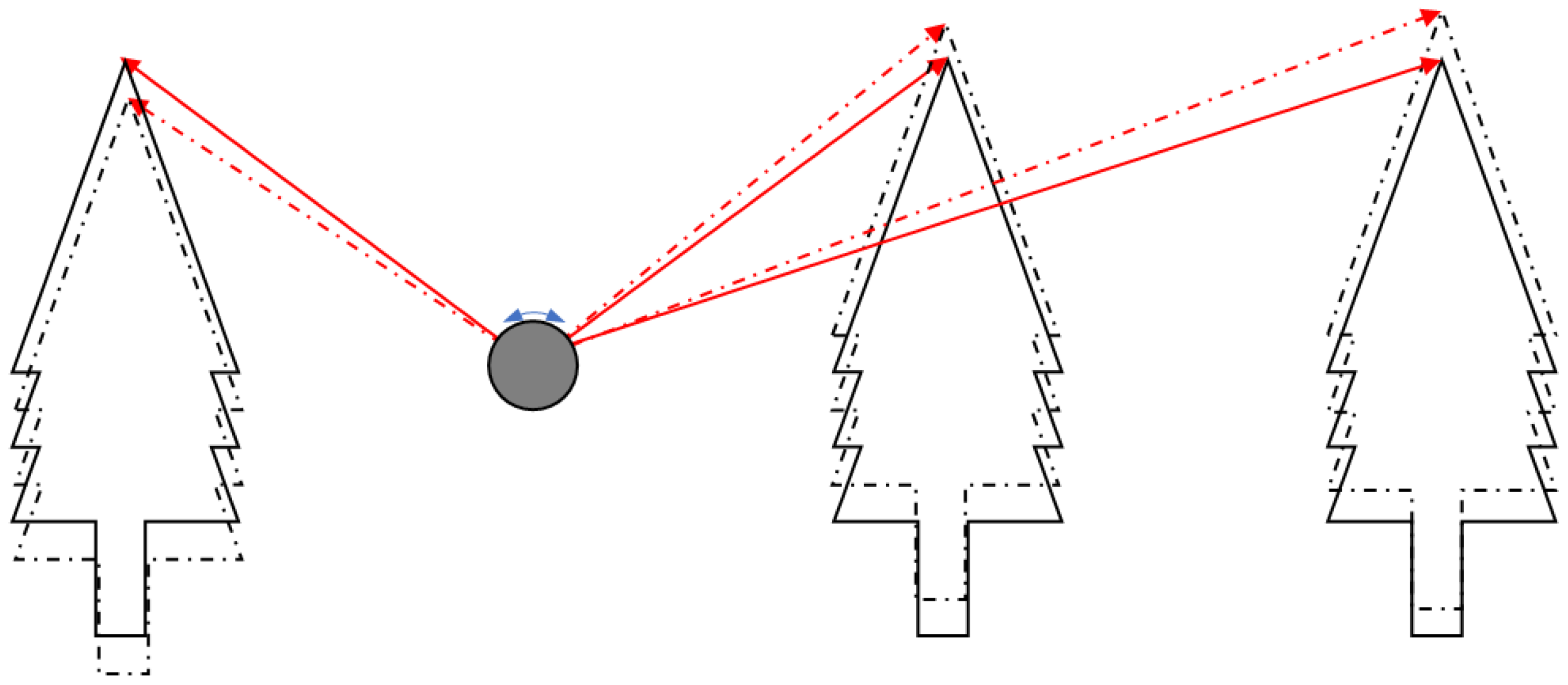
3.1. Measurement of Tree Row Angles

Table 1 shows the angles between the tree rows and the north direction, which represented the actual tree row angles. The actual mean tree row angle was 12.75°, while the estimated angle using the histogram (Figure 8) of heading angles was 12.50°, with an absolute error of only 0.25°.

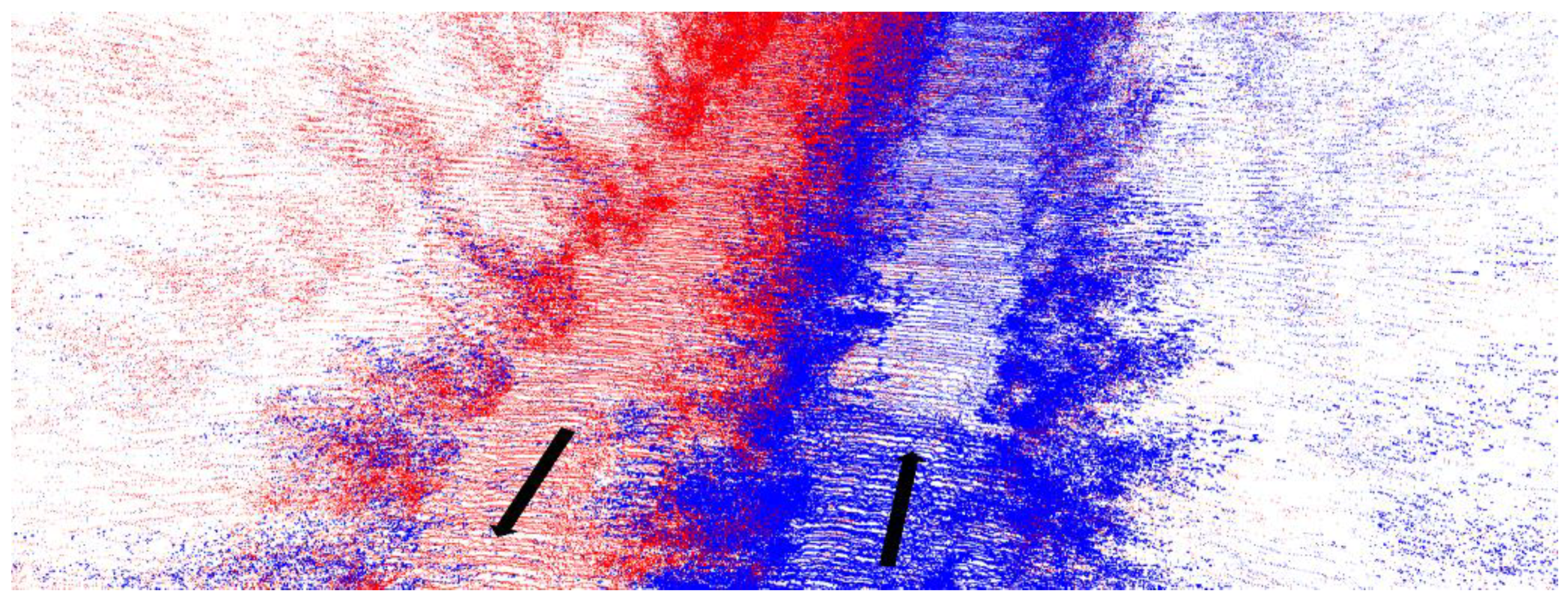
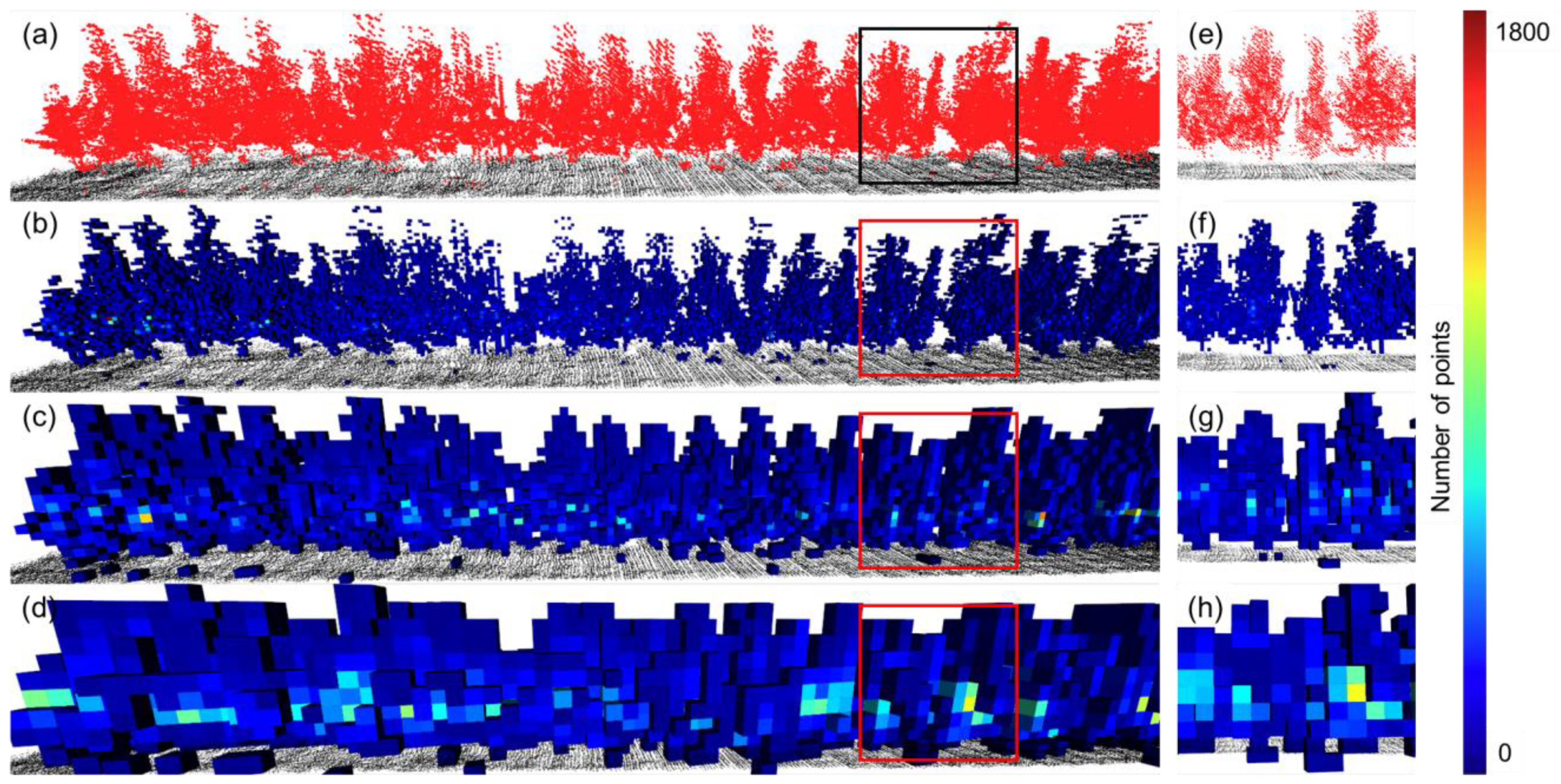
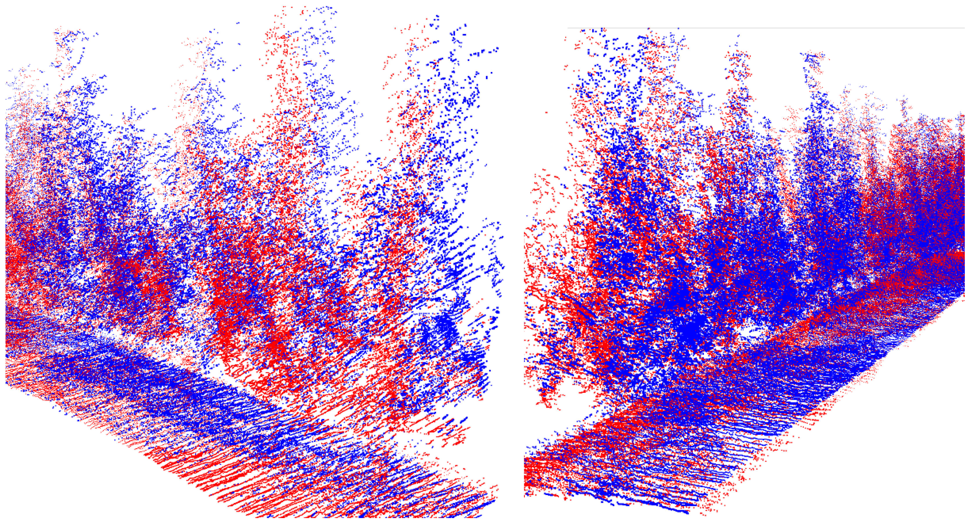
3.2. Visualization of Point Cloud and Voxel Prescription Map

Point clouds scanned from two different trajectories were registered to check for any overlap of point clouds at the same feature locations. The rows of trees were scanned from both sides (Figure 9) and were shown in red and blue, respectively. Due to the slope of the laser lines and the gaps between the trees, the LiDAR was able to scan the trees in the behind rows.
The canopy details facing the driving path were well represented in the point cloud. The branches and details of the canopy on the side away from the driving path were not abundant due to shading of the branches and leaves inside the canopy. The point clouds of the two scans at the treetops basically overlapped, indicating that the point cloud accuracy based on LiDAR-RTK fusion could meet the application requirements.
Voxelization is a method to reduce the amount of data in point cloud processing, and the key parameter is voxel size. The space required to store a voxel prescription map increases exponentially as the voxel size decreases. Although too small a voxel size preserves more crown detail, it increases the memory space and traversal lookup overhead and also takes longer to generate the prescription map. Because of the diffusion of droplets, variable sprays are difficult to perform according to very small voxel intervals. The complexity of the algorithm needs to be balanced with the accuracy of the canopy resolution, so, in this study, the prescription maps were constructed with voxel sizes of 0.1 m, 0.25 m, and 0.5 m, respectively.
As shown in Figure 10b, the prescription map with a voxel side length of 0.1 m contained abundant details. Although the prescription map was generated by limiting the minimum number of points in each cell, there were still more isolated voxels, possibly noisy points and mis-segmented ground. The prescription map with a voxel side length of 0.25 m also contained sufficient information, and the gaps between trees and the height of the trees were still clearly visible, Figure 10c. However, when the voxel size rises to 0.5 m, inter-tree gaps and branches were already difficult to detect, Figure 10d,h. Variable rate spraying determines the number of nozzles to open based primarily on the height of the tree and turns off spraying in the gaps between trees to conserve pesticides and reduce drift pollution.

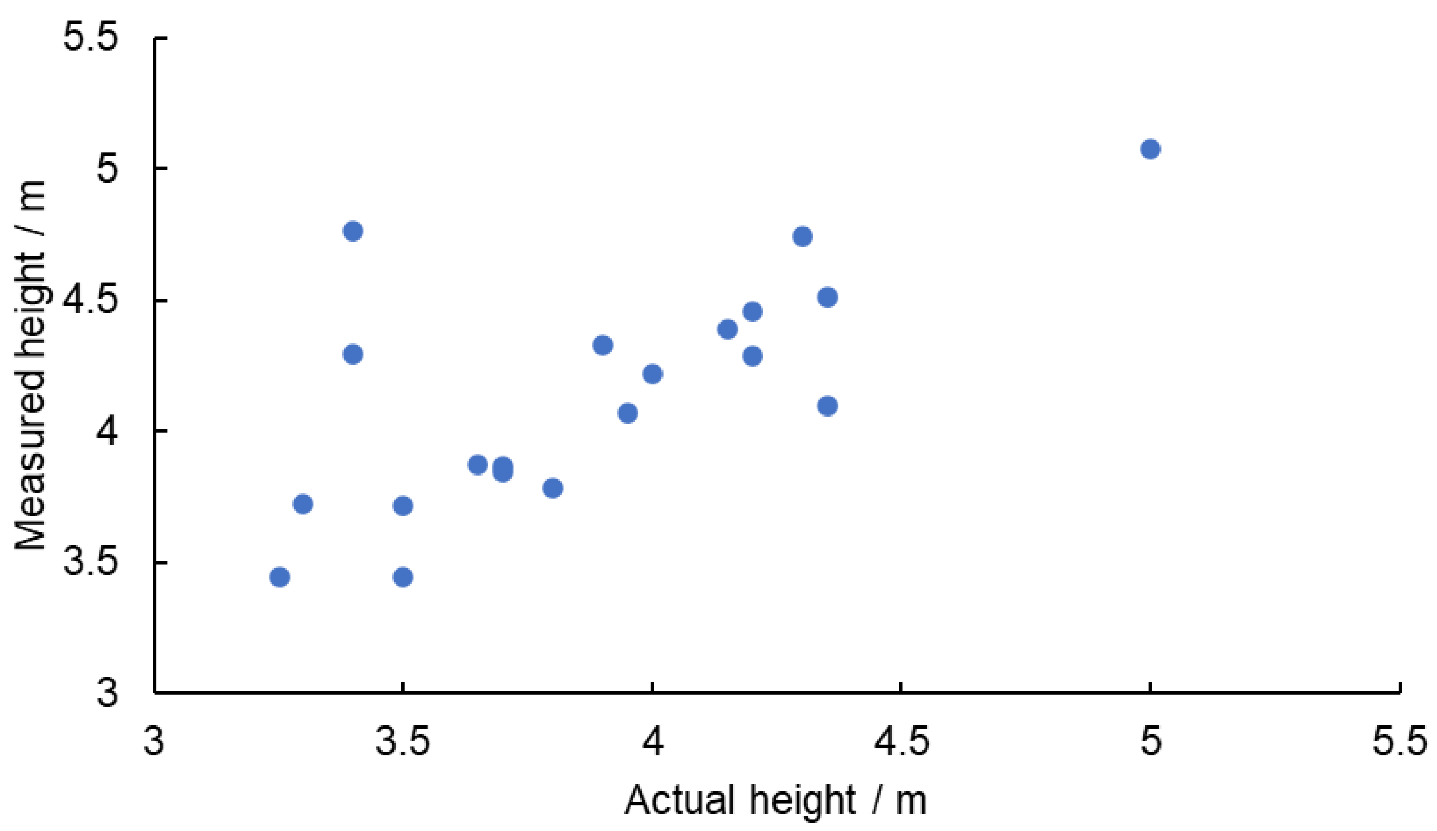
3.3. Accuracy of Tree Height Measurements

The true heights of 20 trees were measured, with a mean height of 3.86 m. The actual tree heights were mainly concentrated in the range of 3.0–4.5 m, and the measurement error was larger for trees with heights less than 3.5 m (Figure 11). This may be caused by adjacent taller branches growing over the lower trees, causing measurement errors. The RMSE between the laser-measured and actual tree heights was 0.42 m, with an rRMSE of 10.86% and an MAPE of 8.16%. This proved the accuracy of the stitching and reconstruction of the LiDAR point cloud.

4. Discussion

When the LiDAR-RTK fusion data acquisition system travels through orchards, the canopy was scanned multiple times from different angles. The point cloud obtained from directly stitching the point clouds based on RTK coordinate transformation was acceptable for the digital management, such as the pesticide applications. The outer canopy closer to the LiDAR was more likely to intercept and reflect more laser because the LiDAR lasers do not penetrate the leaves. Therefore, at least two directions were required to obtain sufficient canopy detail. The tests were conducted in a flat orchard, and the point cloud stitching assumed that the LIDAR had only yaw angle and no cross-roll or pitch motion. However, during the actual scanning process, the point clouds from multiple scans may not be perfectly aligned because the ATV was bumpy due to potholes or uneven ground (Figure 12). This can be improved in the future by using an IMU for attitude correction of roll and pitch angles.
Due to the uneven ground in mountain orchards, the LIDAR attitude is deflected [32], resulting in measurement errors that increase with detection distance (Figure 13). For continuous deflection in smooth motion, where both the ground and tree point clouds appear to be deflected, using the tree height minus ground height method will still give an accurate tree height. However, for shorter target trees, if a taller branch of an adjacent tree extended above the target tree, the additional branch was considered part of the target tree, resulting in a larger height error. More statistical indicators, such as quartiles, may be used to improve the accuracy.
Compared to real-time variable-rate spray systems based on ultrasound or LiDAR, a variable spray system based on prescription maps only requires precise positioning and spray control systems, without the need for expensive sensors on each machine. Remote measurement of canopy height and volume using UAV and SFM algorithms has been applied in various fields. Changes in drone flight parameters may result in the inability to complete reconstruction using the digital surface model, leading to an RMSE of tree height measurements of up to 2.7 m [23]. However, ground-based information collection equipment is still required to obtain detailed information below the canopy [33]. Ground-based methods can provide more details than UAV-based methods [28]. Real-time simultaneous localization and mapping (SLAM) based on LiDAR has been widely researched in urban scenes, achieving satisfactory mapping results. However, in an unstructured orchard, it may be difficult to extract feature points, and the matching may not converge [34,35]. Offline computing methods have no real-time requirements and can be used to extract more features and use more complex algorithms to achieve better registration.
Additionally, real-time variable spray decision-making requires powerful computers due to the complex image and LiDAR processing. The LiDAR-RTK fusion data acquisition system developed in this study obtained voxel canopy volume data with geographic information by driving though the orchard, which can be shared with multiple machines to improve application efficiency. The constructed voxel prescription map can be used to make on–off decisions, such as turning off spraying in areas without canopy cover to reduce pesticide pollution and drift. Using Voxel R-CNN for obstacle detection has the potential to implement semantic maps [36]. The voxel prescription map also includes point-count information, which can be used to determine leaf density [19,37] for pruning [38] and pesticide application for more precise spray and airflow control. The LiDAR-RTK fusion information acquisition system is installed on an electric ATV with autonomous driving system enabling automated acquisition of orchard canopy information.

5. Conclusions

A LiDAR-RTK fusion data acquisition system was developed, which is easy to implement, and deployed on an ATV with autonomous driving system which can be used for canopy point cloud scanning autonomously. This system was tested in a pear orchard to evaluate the accuracy of the voxel prescription map. The position and height of 20 trees were measured, and the absolute error between the estimated tree row angle based on the heading angle histogram and the actual angle was 0.25°. The RMSE of the tree height measured by the LiDAR point cloud and the actual tree height was 0.42 m, with an rRMSE of 10.86% and a MAPE of 8.16%. The prescription map with a voxel side length of 0.25 m contained sufficient canopy detail information and indirectly reflected leaf density in each voxel, which made it suitable for precision management of orchards, such as precise pesticide application and recommendation for pruning operations. This system provides a demonstration for unmanned digital information acquisition in orchards.

Author Contributions

L.H.: Conceptualization, Investigation, Methodology, Validation, Writing—original draft. S.W.: Conceptualization, Investigation, Writing—review and editing. Z.W.: Conceptualization, Investigation, Writing—review and editing. L.J.: Conceptualization, Investigation, Methodology, Validation. X.H.: Supervision, Funding acquisition. All authors have read and agreed to the published version of the manuscript.

Funding

Supported by the earmarked fund for China Agriculture Research System (CARS-28), the 2115 talent development program of China Agricultural University and Sanya Institute of China Agricultural University Guiding Fund Project, Grant No. SYND-2021-06.

Data Availability Statement

Not applicable.

Conflicts of Interest

The authors declare no conflict of interest. The funders had no role in the design of the study; in the collection, analyses, or interpretation of data; in the writing of the manuscript; or in the decision to publish the results.

References

  1. Duga, A.T.; Ruysen, K.; Dekeyser, D.; Nuyttens, D.; Bylemans, D.; Nicolai, B.M.; Verboven, P. Spray Deposition Profiles in Pome Fruit Trees: Effects of Sprayer Design, Training System and Tree Canopy Characteristics. Crop Prot. 2015, 67, 200–213. [Google Scholar] [CrossRef]
  2. Zhu, H.; Brazee, R.D.; Derksen, R.C.; Fox, R.D.; Krause, C.R.; Ozkan, H.E.; Losely, K. Specially Designed Air-Assisted Sprayer to Improve Spray Penetration and Air Jet Velocity Distribution Inside Dense Nursery Crops. Trans. ASABE 2006, 49, 1285–1294. [Google Scholar] [CrossRef]
  3. De Cock, N.; Massinon, M.; Salah, S.O.T.; Lebeau, F. Investigation on Optimal Spray Properties for Ground Based Agricultural Applications Using Deposition and Retention Models. Biosyst. Eng. 2017, 162, 99–111. [Google Scholar] [CrossRef] [Green Version]
  4. Gentil-Sergent, C.; Basset-Mens, C.; Gaab, J.; Mottes, C.; Melero, C.; Fantke, P. Quantifying Pesticide Emission Fractions for Tropical Conditions. Chemosphere 2021, 275, 130014. [Google Scholar] [CrossRef] [PubMed]
  5. Grella, M.; Marucco, P.; Manzone, M.; Gallart, M.; Balsari, P. Effect of Sprayer Settings on Spray Drift during Pesticide Application in Poplar Plantations (Populus Spp.). Sci. Total Environ. 2017, 578, 427–439. [Google Scholar] [CrossRef] [Green Version]
  6. Hong, S.-W.; Zhao, L.; Zhu, H. CFD Simulation of Pesticide Spray from Air-Assisted Sprayers in an Apple Orchard: Tree Deposition and off-Target Losses. Atmos. Environ. 2018, 175, 109–119. [Google Scholar] [CrossRef]
  7. Sinha, R.; Ranjan, R.; Khot, L.R.; Hoheisel, G.; Grieshop, M.J. Drift Potential from a Solid Set Canopy Delivery System and an Axial–Fan Air–Assisted Sprayer during Applications in Grapevines. Biosyst. Eng. 2019, 188, 207–216. [Google Scholar] [CrossRef]
  8. Rathnayake, A.P.; Chandel, A.K.; Schrader, M.J.; Hoheisel, G.A.; Khot, L.R. Spray Patterns and Perceptive Canopy Interaction Assessment of Commercial Airblast Sprayers Used in Pacific Northwest Perennial Specialty Crop Production. Comput. Electron. Agric. 2021, 184, 106097. [Google Scholar] [CrossRef]
  9. Otto, S.; Loddo, D.; Baldoin, C.; Zanin, G. Spray Drift Reduction Techniques for Vineyards in Fragmented Landscapes. J. Environ. Manag. 2015, 162, 290–298. [Google Scholar] [CrossRef]
  10. Garcerá, C.; Doruchowski, G.; Chueca, P. Harmonization of Plant Protection Products Dose Expression and Dose Adjustment for High Growing 3D Crops: A Review. Crop Prot. 2021, 140, 105417. [Google Scholar] [CrossRef]
  11. Zaman, Q.U.; Esau, T.J.; Schumann, A.W.; Percival, D.C.; Chang, Y.K.; Read, S.M.; Farooque, A.A. Development of Prototype Automated Variable Rate Sprayer for Real-Time Spot-Application of Agrochemicals in Wild Blueberry Fields. Comput. Electron. Agric. 2011, 76, 175–182. [Google Scholar] [CrossRef]
  12. Gil, E.; Llorens, J.; Llop, J.; Fàbregas, X.; Escolà, A.; Rosell-Polo, J.R. Variable Rate Sprayer. Part 2–Vineyard Prototype: Design, Implementation, and Validation. Comput. Electron. Agric. 2013, 95, 136–150. [Google Scholar] [CrossRef] [Green Version]
  13. Llorens, J.; Gil, E.; Llop, J.; Escolà, A. Ultrasonic and LIDAR Sensors for Electronic Canopy Characterization in Vineyards: Advances to Improve Pesticide Application Methods. Sensors 2011, 11, 2177–2194. [Google Scholar] [CrossRef] [PubMed] [Green Version]
  14. Nan, Y.; Zhang, H.; Zheng, J.; Bian, L.; Li, Y.; Yang, Y.; Zhang, M.; Ge, Y. Estimating Leaf Area Density of Osmanthus Trees Using Ultrasonic Sensing. Biosyst. Eng. 2019, 186, 60–70. [Google Scholar] [CrossRef]
  15. Palleja, T.; Landers, A.J. Real Time Canopy Density Validation Using Ultrasonic Envelope Signals and Point Quadrat Analysis. Comput. Electron. Agric. 2017, 134, 43–50. [Google Scholar] [CrossRef]
  16. Liu, L.; Liu, Y.; He, X.; Liu, W. Precision Variable-Rate Spraying Robot by Using Single 3D LIDAR in Orchards. Agronomy 2022, 12, 2509. [Google Scholar] [CrossRef]
  17. Salcedo, R.; Zhu, H.; Ozkan, E.; Falchieri, D.; Zhang, Z.; Wei, Z. Reducing Ground and Airborne Drift Losses in Young Apple Orchards with PWM-Controlled Spray Systems. Comput. Electron. Agric. 2021, 189, 106389. [Google Scholar] [CrossRef]
  18. Hu, M.; Whitty, M. An Evaluation of an Apple Canopy Density Mapping System for a Variable-Rate Sprayer. IFAC-PapersOnLine 2019, 52, 342–348. [Google Scholar] [CrossRef]
  19. Sultan Mahmud, M.; Zahid, A.; He, L.; Choi, D.; Krawczyk, G.; Zhu, H.; Heinemann, P. Development of a LiDAR-Guided Section-Based Tree Canopy Density Measurement System for Precision Spray Applications. Comput. Electron. Agric. 2021, 182, 106053. [Google Scholar] [CrossRef]
  20. Li, Q.; Xue, Y. Total Leaf Area Estimation Based on the Total Grid Area Measured Using Mobile Laser Scanning. Comput. Electron. Agric. 2023, 204, 107503. [Google Scholar] [CrossRef]
  21. Manandhar, A.; Zhu, H.; Ozkan, E.; Shah, A. Techno-Economic Impacts of Using a Laser-Guided Variable-Rate Spraying System to Retrofit Conventional Constant-Rate Sprayers. Precis. Agric. 2020, 21, 1156–1171. [Google Scholar] [CrossRef]
  22. Pfeiffer, S.A.; Guevara, J.; Cheein, F.A.; Sanz, R. Mechatronic Terrestrial LiDAR for Canopy Porosity and Crown Surface Estimation. Comput. Electron. Agric. 2018, 146, 104–113. [Google Scholar] [CrossRef]
  23. Kameyama, S.; Sugiura, K. Estimating Tree Height and Volume Using Unmanned Aerial Vehicle Photography and SfM Technology, with Verification of Result Accuracy. Drones 2020, 4, 19. [Google Scholar] [CrossRef]
  24. Mahmud, M.S.; He, L.; Heinemann, P.; Choi, D.; Zhu, H. Unmanned Aerial Vehicle Based Tree Canopy Characteristics Measurement for Precision Spray Applications. Smart Agric. Technol. 2023, 4, 100153. [Google Scholar] [CrossRef]
  25. Sinha, R.; Quirós, J.J.; Sankaran, S.; Khot, L.R. High Resolution Aerial Photogrammetry Based 3D Mapping of Fruit Crop Canopies for Precision Inputs Management. Inf. Process. Agric. 2022, 9, 11–23. [Google Scholar] [CrossRef]
  26. Brocks, S.; Bendig, J.; Bareth, G. Toward an Automated Low-Cost Three-Dimensional Crop Surface Monitoring System Using Oblique Stereo Imagery from Consumer-Grade Smart Cameras. J. Appl. Remote Sens. 2016, 10, 046021. [Google Scholar] [CrossRef] [Green Version]
  27. Jay, S.; Rabatel, G.; Hadoux, X.; Moura, D.; Gorretta, N. In-Field Crop Row Phenotyping from 3D Modeling Performed Using Structure from Motion. Comput. Electron. Agric. 2015, 110, 70–77. [Google Scholar] [CrossRef] [Green Version]
  28. Andújar, D.; Moreno, H.; Bengochea-Guevara, J.M.; de Castro, A.; Ribeiro, A. Aerial Imagery or On-Ground Detection? An Economic Analysis for Vineyard Crops. Comput. Electron. Agric. 2019, 157, 351–358. [Google Scholar] [CrossRef]
  29. Pierzchała, M.; Giguère, P.; Astrup, R. Mapping Forests Using an Unmanned Ground Vehicle with 3D LiDAR and Graph-SLAM. Comput. Electron. Agric. 2018, 145, 217–225. [Google Scholar] [CrossRef]
  30. Ji, Y.; Li, S.; Peng, C.; Xu, H.; Cao, R.; Zhang, M. Obstacle Detection and Recognition in Farmland Based on Fusion Point Cloud Data. Comput. Electron. Agric. 2021, 189, 106409. [Google Scholar] [CrossRef]
  31. Meier, U.; Bleiholder, H.; Buhr, L.; Feller, C.; Hack, H.; Heß, M.; Lancashire, P.; Schnock, U.; Stauß, R.; Van den Boom, T.; et al. The BBCH System to Coding the Phenological Growth Stages of Plants-History and Publications. J. Kult. 2009, 61, 41–52. [Google Scholar] [CrossRef]
  32. Mahmud, S.; Zahid, A.; He, L.; Choi, D.; Krawczyk, G. LiDAR-Sensed Tree Canopy Correction in Uneven Terrain Conditions Using a Sensor Fusion Approach for Precision Sprayers. Comput. Electron. Agric. 2021, 191, 106565. [Google Scholar] [CrossRef]
  33. Torresan, C.; Carotenuto, F.; Chiavetta, U.; Miglietta, F.; Zaldei, A.; Gioli, B. Individual Tree Crown Segmentation in Two-Layered Dense Mixed Forests from UAV LiDAR Data. Drones 2020, 4, 10. [Google Scholar] [CrossRef] [Green Version]
  34. Chen, X.; Wang, S.; Zhang, B.; Luo, L. Multi-Feature Fusion Tree Trunk Detection and Orchard Mobile Robot Localization Using Camera/Ultrasonic Sensors. Comput. Electron. Agric. 2018, 147, 91–108. [Google Scholar] [CrossRef]
  35. Garforth, J.; Webb, B. Visual Appearance Analysis of Forest Scenes for Monocular SLAM. In Proceedings of the 2019 International Conference on Robotics and Automation (ICRA), Montreal, QC, Canada, 20–27 May 2019; IEEE: Piscataway, NJ, USA, 2019; pp. 1794–1800. [Google Scholar]
  36. Qin, J.; Sun, R.; Zhou, K.; Xu, Y.; Lin, B.; Yang, L.; Chen, Z.; Wen, L.; Wu, C. Lidar-Based 3D Obstacle Detection Using Focal Voxel R-CNN for Farmland Environment. Agronomy 2023, 13, 650. [Google Scholar] [CrossRef]
  37. Berk, P.; Stajnko, D.; Belsak, A.; Hocevar, M. Digital Evaluation of Leaf Area of an Individual Tree Canopy in the Apple Orchard Using the LIDAR Measurement System. Comput. Electron. Agric. 2020, 169, 105158. [Google Scholar] [CrossRef]
  38. Westling, F.; Underwood, J.; Bryson, M. A Procedure for Automated Tree Pruning Suggestion Using LiDAR Scans of Fruit Trees. Comput. Electron. Agric. 2021, 187, 106274. [Google Scholar] [CrossRef]
Figure 1. LiDAR-RTK fusion data acquisition system and data processing algorithm.
Drones 07 00242 g001
Figure 2. (a) Location of the experimental orchard; (b) Pear trees in orchard.
Drones 07 00242 g002
Figure 3. The LiDAR-RTK fusion data acquisition system is fixed on an ATV which can automatically traverse along the pre-determined trajectory.
Drones 07 00242 g003
Figure 4. LiDAR field of view at different mounting angles. (a) The range of view of the LiDAR when mounted horizontally and vertically. (b) The range of view when the LiDAR is mounted at 45°.
Drones 07 00242 g004
Figure 5. Dual antenna RTK rover can acquire position and heading angle.
Drones 07 00242 g005
Figure 6. Different coordinate system in the LiDAR-RTK fusion data acquisition system.
Drones 07 00242 g006
Figure 7. (a) Measurement of tree position by handheld tilt-featured RTK receiver. (b) Measuring the height of trees by means of a tower ruler.
Drones 07 00242 g007
Figure 8. Histogram of heading angles.
Drones 07 00242 g008
Figure 9. The original point cloud of tree rows scanned from different sides; the red and blue points are scanned from different sides, and the black arrows identify the direction of travel.
Drones 07 00242 g009
Figure 10. Prescription maps of tree row: (a) scanned raw point cloud with canopy points in red and ground points in black; (bd) prescription map with voxel size of 0.1 m, 0.25 m, 0.5 m, respectively, and the color of each voxel represents the number of points contained within it; (e) scanned raw point cloud of the gap between the trees; (fh) detail of the prescription map, respectively.
Drones 07 00242 g010
Figure 11. The actual height of the target tree and the height measured from the point cloud.
Drones 07 00242 g011
Figure 12. Detail of the original point cloud scanned from both sides; the red and blue points are scanned from each side.
Drones 07 00242 g012
Figure 13. Measurement errors of tree height increase with the detection distance due to the roll angle of the LiDAR.
Drones 07 00242 g013
Table 1. The angle of the tree rows fitted from the measured tree position.
Actual Tree Row Angle/°MeanStandard Deviation
123456
12.9012.7112.6012.4913.0312.7712.750.198
Disclaimer/Publisher’s Note: The statements, opinions and data contained in all publications are solely those of the individual author(s) and contributor(s) and not of MDPI and/or the editor(s). MDPI and/or the editor(s) disclaim responsibility for any injury to people or property resulting from any ideas, methods, instructions or products referred to in the content.

