Spectral-Spatial Attention Rotation-Invariant Classification Network for Airborne Hyperspectral Images

Abstract

An airborne hyperspectral imaging system is typically equipped on an aircraft or unmanned aerial vehicle (UAV) to capture ground scenes from an overlooking perspective. Due to the rotation of the aircraft or UAV, the same region of land cover may be imaged from different viewing angles. While humans can accurately recognize the same objects from different viewing angles, classification methods based on spectral-spatial features for airborne hyperspectral images exhibit significant errors. The existing methods primarily involve incorporating image or feature rotation angles into the network to improve its accuracy in classifying rotated images. However, these methods introduce additional parameters that need to be manually determined, which may not be optimal for all applications. This paper presents a spectral-spatial attention rotation-invariant classification network for the airborne hyperspectral image to address this issue. The proposed method does not require the introduction of additional rotation angle parameters. There are three modules in the proposed framework: the band selection module, the local spatial feature enhancement module, and the lightweight feature enhancement module. The band selection module suppresses redundant spectral channels, while the local spatial feature enhancement module generates a multi-angle parallel feature encoding network to improve the discrimination of the center pixel. The multi-angle parallel feature encoding network also learns the position relationship between each pixel, thus maintaining rotation invariance. The lightweight feature enhancement module is the last layer of the framework, which enhances important features and suppresses insignificance features. At the same time, a dynamically weighted cross-entropy loss is utilized as the loss function. This loss function adjusts the model’s sensitivity for samples with different categories according to the output in the training epoch. The proposed method is evaluated on five airborne hyperspectral image datasets covering urban and agricultural regions. Compared with other state-of-the-art classification algorithms, the method achieves the best classification accuracy and is capable of effectively extracting rotation-invariant features for urban and rural areas.

1. Introduction

With the development of optical imaging technology and unmanned aerial vehicle (UAV) technology, airborne hyperspectral imaging (HSI) has become increasingly abundant. HSI differs from RGB images in that it contains a large amount of spectral and spatial information. The continuous spectral curve of HSI can identify various objects, as different objects have different spectral curves [1]. As a result, the airborne hyperspectral image has been widely used in applications such as urban planning [2], agricultural monitoring [3], disaster detection [4].

Table 1. The common airborne hyperspectral images datasets.

Dataset	Sensor	Platform	Bands	Range (nm)	Land-Cover	Area
Indian Pines	AVIRIS	Aerial	220	400–2500	16	Agriculture
Luojia-HSSR [5]	AMMHS	Aerial	249	390–980	23	Urban
Houston	ITERS CASI	Aerial	144	364–1046	15	Urban
Pavia Center	ROSIS	Aerial	102	430–860	9	Urban
Matiwan [6]	VNIR	UAV	250	400–1000	13	Agriculture
WHU-Hi-Longkou	Headwall	UAV	270	400–1000	9	Agriculture
WHU-Hi-HanChuan	Headwall	UAV	270	400–1000	16	Agriculture
WHU-Hi-HongHu	Headwall	UAV	270	400–1000	22	Agriculture

shows the common airborne hyperspectral image datasets captured by UAVs or aircraft covering urban and agricultural areas.

HSI classification aims to predict the corresponding category for each pixel. Based on how features are extracted, HSI classification methods are roughly divided into traditional and deep learning methods. The traditional methods [7,8] typically extract hyperspectral spatial-spectral features using handcrafted features, followed by a feature-classifying module. This paper [7] proposed using Independent Component Discriminant Analysis (ICDA) for classification. Cao et al. [9] used the three-dimensional discrete wavelet transform (3D-DWT) to extract the spatial-spectral feature for HSI classification. While traditional methods [10,11,12] have achieved good results, the handcrafted features are generally shallow features with limited feature representation capability, making it challenging to achieve satisfactory performance.

In recent years, deep learning methods have been the mainstream approach in HSI classification [13]. Hyperspectral images contain rich spectral information, with each category having unique spectral information [1]. Based on the different information methods, deep learning methods are broadly divided into two categories: spectral feature methods [14,15,16] and spectral-spatial feature methods [17,18,19].

Spectral feature algorithms extract features along the 1D spectral dimension. For instance, Chen et al. [20] first applied deep learning to HSI classification. According to Hu et al.’s research [14], 1D convolution neural networks (CNNs) were employed to classify HSI based on spectral features. A novel recurrent neural network (RNN) module [21] was employed in HSI classification. Wu et al. [15] developed an RNN-based semi-supervised classifier for HSI classification. Hang et al. [22] utilized cascaded RNNs for HSI classification. This work used RNNs to model the sequence and effectively represent the relationship between adjacent spectral bands. However, while the spectral dimension can distinguish different land-cover categories, adjacent pixels in HSI may belong to the same land-cover categories [23,24].

In order to achieve an accurate classification of land-cover classes, it is necessary to consider both spectral and spatial features [25]. The spatial-spectral feature methods [19,26,27] have been proposed to address the issues associated with spectral feature methods. For example, Zhang et al. [4] employed a method of learning contextual interaction features using inputs based on different regions. Song et al. [28] introduced residual learning and fused the output of the hierarchical features for HSI classification. To expedite the forward progression of 2D CNN, Mei et al. [18] proposed a novel step activation quantization method. Since HSIs are 3D cubes, 3D CNN has been employed for HSI classification. Wei et al. [29] utilized the edge-preserving sied window filters as the convolution kernels. He et al. [30] proposed a multiscale 3D CNN for classification. A hybrid network [31] that combines 2D CNN and 3D CNN was presented to issue the classification of HSIs. Mei et al. [17] employed an unsupervised 3D CNN autoencoder for HSI classification. Multiple spectral resolution 3D CNN [32] has also been introduced for classification. In addition, attention modules have been embedded in the network to extract spectral-spatial features in HSIs. Zheng et al. [13] proposed an attention mechanism to suppress redundant bands and improve classification accuracy. A novel spectral-spatial attention network [26] was introduced to capture the correlation of the pixels. In most cases [33,34,35,36], these attention modules are independent. This means these modules are flexibly put into the network.

HSIs contain rich spectral information. Meanwhile, the 2D convolution neural networks have significantly affected computer vision, with applications including biomedical image classification [37], remote sensing image classification [3,38], change detection [39,40], and image deblurring [2]. However, when convolving along the spectral dimension of HSI, hundreds of bands need plenty of parameters. There is no doubt that this dramatically increases computational time and cost. The number of channels is usually reduced before using 2D convolution kernels for feature extraction and classification to solve this problem. The mainstream methods include two main types. One is to reduce the spectral dimension. For instance, [31,41] used PCA [42] and variants of PCA [16] to reduce the number of spectral channels. The authors of [43] utilized the enhancing transformation reduction (ETR) for reducing dimensionality and HSI classification. Another option is to suppress the redundant bands using spectral attention methods [25,26]. The spectral attention methods usually change the weights of each band.

The vision transformer (ViT) [44] has recently performed remarkably on some vision-related tasks. As a result, some studies [45,46,47] have attempted to apply ViT to hyperspectral classification. For instance, a novel local transformer [48] with an integrated spatial partition restore module is proposed for classification. He et al. [49] utilized a spatial-spectral transformer with a dense connection, which was proposed to capture sequential spectra relationships. Extended morphological profiles [50] were employed for HSI classification in a deep global-local transformer network. These transformer methods [50,51,52,53] process the hyperspectral images in a token style. Generally, the 3D HSI is divided into patches and treated as tokens. The transformer network extracts the features and relationships of these tokens for hyperspectral classification.

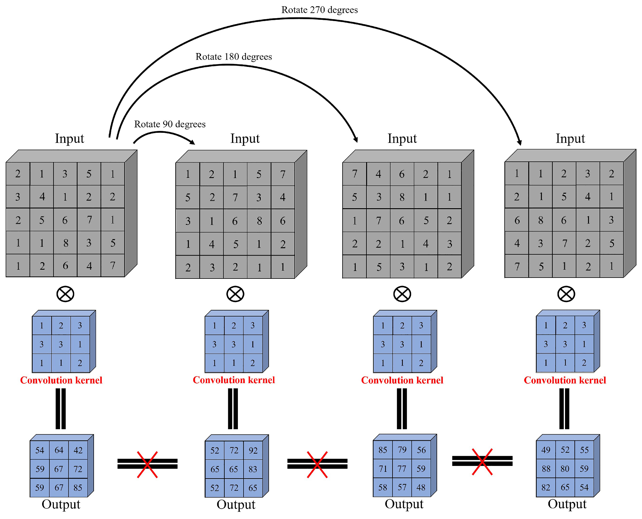
An airborne hyperspectral imaging system is typically equipped on an aircraft or UAV to capture ground scenes from an overlooking perspective. As a result of the rotation of the UAV, the HSI in the same area has different perspectives [13]. While spatial rotation does not typically cause degradation of classification accuracy for spectral-based methods, spectral feature methods do not perform as well as spectral-spatial feature methods, which are sensitive to spatial rotation, as shown in Figure 1. For convenience, the input is set to have one spectral band. The kernel size is $3\times 3$. The image size is $5\times 5$. The stride and padding of convolution are 1 and 0, respectively. Figure 1 shows that different features are extracted from the same image with different input angles using the same convolutional kernel. transformer-based methods face similar problems. The input image rotation causes a change in the output. Therefore, the spatial-spectral methods perform poorly when the images are rotated. In order to address this issue, some work has made meaningful attempts to explore it. Tao et al. [54] utilized vector sorting to extract rotation-invariant features. Zheng et al. [13] used spectral convolution to extract spatial features to maintain rotation invariance. Chen et al. [55] presented using feature rotation to address the rotation invariance of UAV images. 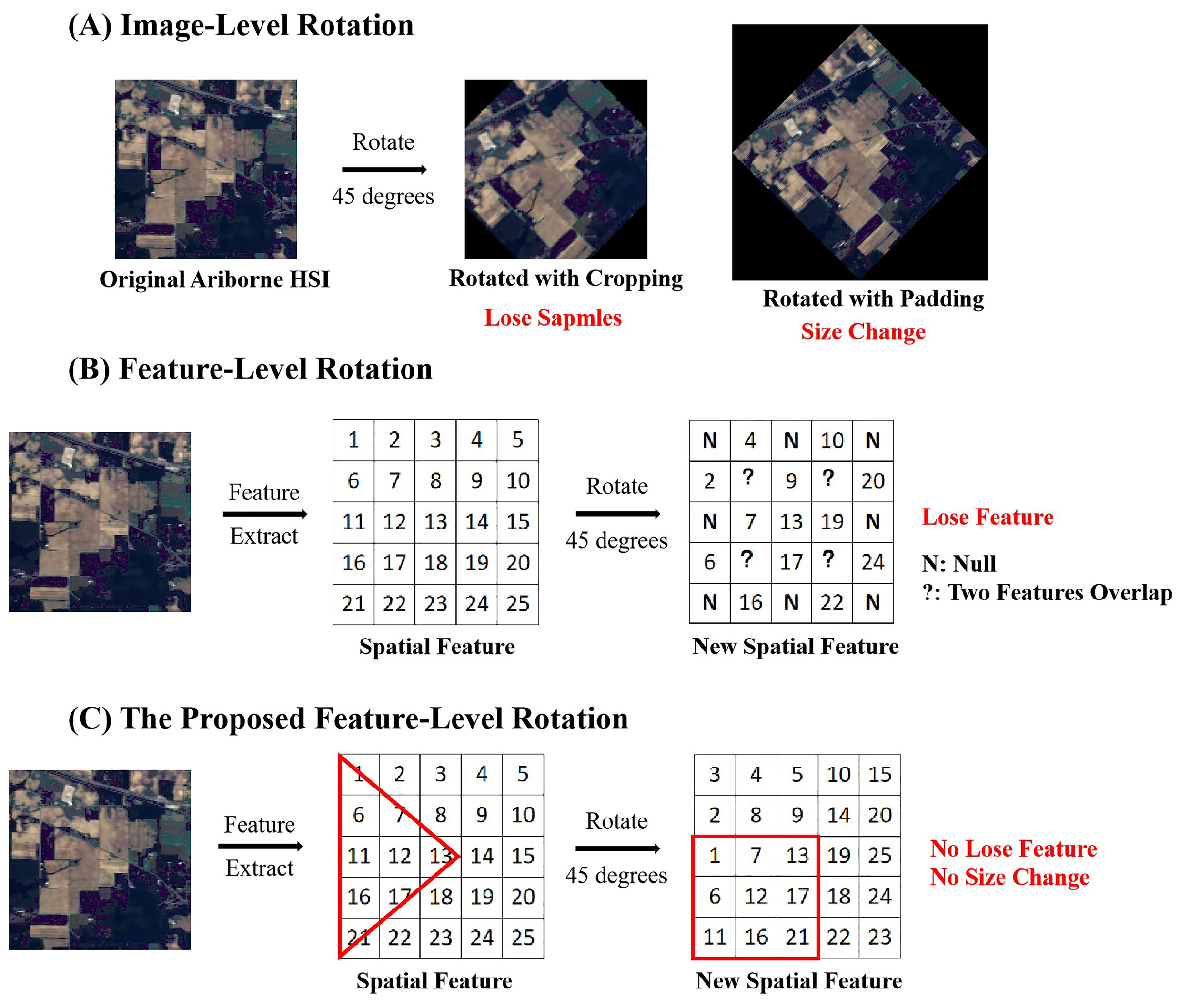Figure 2 illustrates common methods for addressing rotation invariance. Figure 2A shows that the image-level rotation may lose samples or changes the image size. According to [55], the coordinates of each feature are $(x,y)$. The rotation by $\theta$ degrees is expressed as:

$$\begin{array}{c}\hfill \tilde{x}=x\cos \theta -y\sin \theta \\ \hfill \tilde{\mathrm{y}}=x\sin \theta +y\cos \theta \end{array}$$

(1)

where $\tilde{x}$ and $\tilde{y}$ denote the new coordinates of the rotated feature. However, without additional constraint conditions, the feature-level rotation may still lose features, which are shown in Figure 2B. For instance, according to Equation (1), the feature at the coordinate position (−2, −2) will be lost after rotation, while the features at the coordinate positions (−2, 0) and (−1, 0) will have the same new coordinate position (−1, −1) after rotation, resulting in two overlapping features. Figure 2C shows that the proposed feature-level rotation is capable of effectively maintaining all features to address the problem of rotational invariance without the introduction of additional conditions.

A spectral-spatial attention rotation-invariant classification network (SSARIN) is presented based on the above issues. The SSARIN can address the issue of spatial rotation sensitivity in spectral-spatial feature methods of HSI classification. SSARIN is composed of a Band Selection (BS) module, a Local Spatial Feature Enhancement (LSFE) module, and a Lightweight Feature Enhancement (LWFE) module. The BS module is the initial component that reduces redundant spectral channels. The LSFE module generates a multi-angle parallel feature encoding network, which enhances the center pixel’s discrimination ability and learns the positional relationship between each pixel, ensuring rotation invariance. The LWFE module enhances significant features and suppresses insignificant ones as the final layer. At the same time, a dynamically weighted cross-entropy loss function is employed.

This paper has the following contributions.

1.

We present spectral-spatial attention rotation-invariant classification network (SSARIN) that utilizes convolutional neural networks (CNNs) to extract spectral-spatial features. The SSARIN not only achieves good performance in HSI classification, but is also a rotation-invariant network. Additionally, a dynamically weighted cross-entropy loss is introduced that considers the complexities of samples with different categories to improve classification accuracy.

2.

A local spatial feature enhancement module is proposed to address the issue of spatial rotation sensitivity. This module not only captures spatial-spectral features but also learns the position relationship between pixels. Doing so enhances the discriminative power of the center pixel and alleviates the impact of spatial rotation on classification accuracy.

The paper is divided into the following sections. Section 2 shows the proposed method in more detail. Section 3 discusses the experimental results. The discussion is presented in Section 4. Finally, a conclusion is drawn in Section 5.

2. Proposed Method

This section describes the various components of the proposed network in detail. The overview of the algorithm is shown in Section 2.1. Section 2.2 contains the details of the band selection module. The local spatial feature enhancement module is explained in Section 2.3. Section 2.4 introduces the lightweight feature enhancement. Finally, the loss function is reported in Section 2.5.

2.1. Overview

The HSI is a 3D cube [26]. Suppose that $\mathbf{X}\in {\mathbb{R}}^{\mathrm{H}\times \mathrm{W}\times \mathrm{B}}$ denotes the HSIs, where $\mathrm{H}\times \mathrm{W}$ represents the spatial size of the image. $\mathrm{B}$ is the number of channels. The $\mathbf{Y}=\left[y_1,y_2,\cdots ,y_c\right]\in {\mathbb{R}}^{1\times 1\times \mathrm{C}}$ represents the land-cover categories. $\mathrm{C}$ denotes the number of classes. The $\mathbf{Y}$ is a one-hot label vector. Classification aims to make each hyperspectral image pixel have a corresponding category.

Let ${\mathbf{X}}_i\in {\mathbb{R}}^{\mathrm{p}\times \mathrm{p}\times \mathrm{b}}$ represent the patch, a square area cut from the HSI ${\mathbf{X}}_p$. ${\mathbf{X}}_p$ represents the hyperspectral image after principal components analysis (PCA). ${\mathbf{X}}_i$ denotes the i-th patch of the hyperspectral image ${\mathbf{X}}_p$. $\mathrm{p}\times \mathrm{p}$ is the spatial size. The pixel ${\mathrm{x}}_i^c$ represents the center pixel of the patch ${\mathbf{X}}_i$. Each pixel has a corresponding patch in the HSIs. Thus, the proposed SSARIN is utilized to determine the class of the pixel ${\mathrm{x}}_i$ based on patch ${\mathbf{X}}_i$.

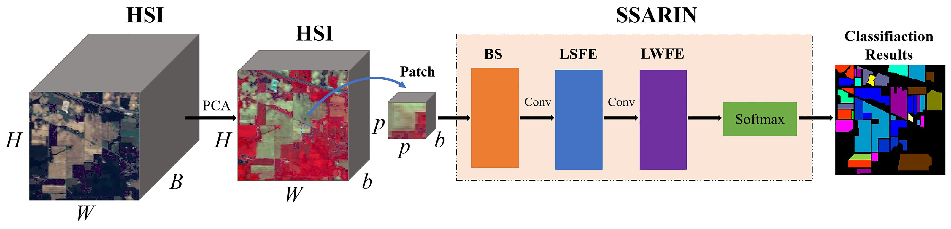
Figure 3 shows the proposed HSI classification method, which mainly contains a band selection (BS) module, a local spatial feature enhancement (LSFE) module, and a lightweight feature enhancement (LWFE) module. Hundreds of bands need many parameters. Many bands are redundant, so PCA can be used to retain the primary spectral information and reduce the number of bands. PCA reduces the number of channels from B to b. In this paper, b is set to 50. Furthermore, a spectral attention mechanism is employed to recalibrate surplus spectral bands. The spectral attention is also named the band selection (BS) in this paper. The HSI patch ${\mathbf{X}}_i\in {\mathbb{R}}^{\mathrm{p}\times \mathrm{p}\times \mathrm{b}}$ is fed into the BS module. This module has the effect of suppressing redundant spectral channels. The main benefits are the following. PCA not only reduces the number of channels but also reduces the number of parameters. The main thing is that the HSIs after PCA retains the primary information. Then, a local spatial feature enhancement module is employed to extract the spectral-spatial features. Meanwhile, the output of the LSFE module consists of rotation-invariant features. Finally, a lightweight feature enhancement is leveraged to enhance essential features, suppressing insignificance features and improving classification accuracy. The core component of SSARIN is the LSFE module.

Table 2. The architecture of the proposed SSARIN.

Module	Layers	Input Size	Output Size	Connected to
Input	Patch H	$P\times P\times B$	/	SpeA, SpeA-Conv
BS	SpeA	$P\times P\times B$	$1\times 1\times B$	SpeA-Conv
	SpeA-Conv	$P\times P\times B$, $1\times 1\times B$	$P\times P\times B$	Rotation
LSFE	Rotation	$P\times P\times B$	$P\times P\times B$	LSFE-Conv-1
	LSFE-Conv-1	$P\times P\times B$	$P\times P\times 256$	SpaA-1, SpaA-Conv-1
	SpaA-1	$P\times P\times 256$	$P\times P\times 1$	SpaA-Conv-1
	SpaA-Conv-1	$P\times P\times 256$, $P\times P\times 1$	$P\times P\times 256$	LSFE-Conv-2
	LSFE-Conv-2	$P\times P\times 256$	$P\times P\times 128$	SpaA-2, SpaA-Conv-2
	SpaA-2	$P\times P\times 128$	$P\times P\times 1$	SpaA-Conv-2
	SpaA-Conv-2	$P\times P\times 128$, $P\times P\times 1$	$P\times P\times 128$	LSFE-Conv-3
	LSFE-Conv-3	$P\times P\times 128$	$K\times K\times 64$	Mean
	Mean	$K\times K\times 64$	$K\times K\times 64$	LSFE-Conv
LWFE	LSFE-Conv	$K\times K\times 64$	$K\times K\times 64$	AP
	AP	$K\times K\times 64$	$1\times 1\times 64$	FC
Classifier	FC	$1\times 1\times 64$	16	LogSoftmax
	LogSoftmax	16	C	/

reports the details of the presented algorithm.

2.2. Band Selection Module

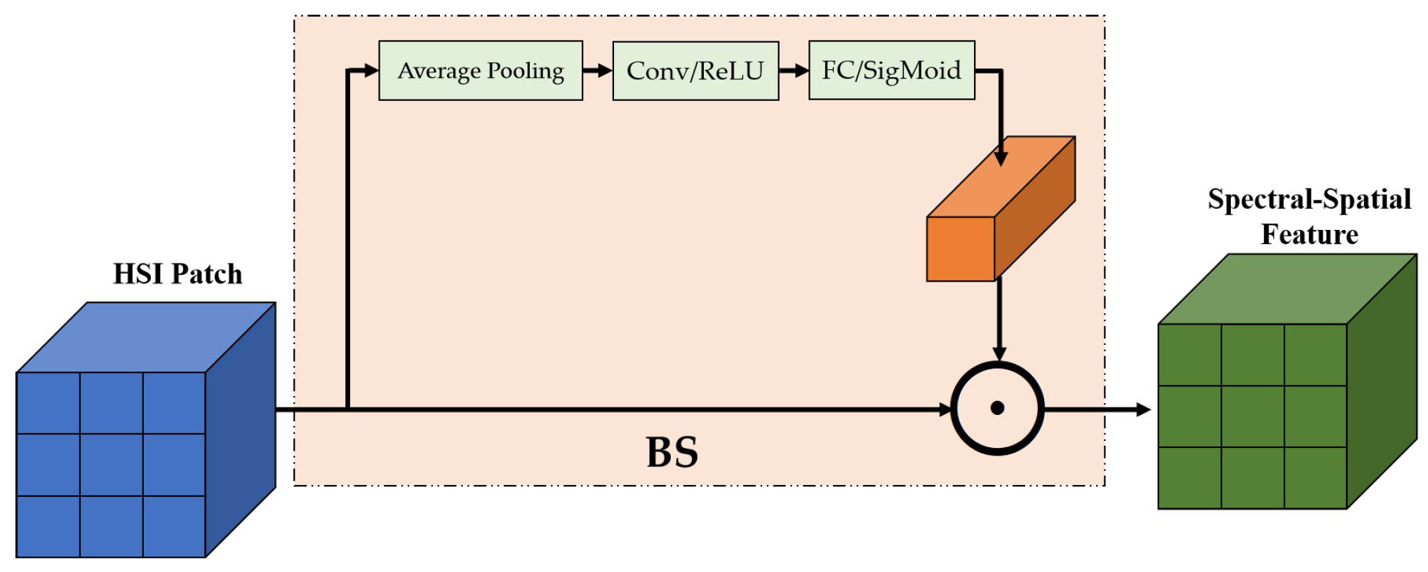
The band selection module contains three layers: one average pooling and two convolution layers. This module emphasizes the useful bands and suppresses the redundant ones by adaptive weights. The BS module recalibrates the spectral bands and adjusts the weight of each band. Figure 4 shows the details of the BS module.

Table 3. The detailed structures of the band selection (BS) module.

Layers	Input Size	Output Size	Kernel Size
AP	$P\times P\times N$	$1\times 1\times N$	/
Conv+ReLU	$1\times 1\times N$	$1\times 1\times N/4$	$1\times 1\times N/4$
Conv	$1\times 1\times N/4$	$1\times 1\times N$	$1\times 1\times N$
$\sigma \left(·\right)$	$1\times 1\times N$	$1\times 1\times N$	/
⊙	$1\times 1\times N$/$P\times P\times N$	$P\times P\times N$	/

lists detailed information on the BS module. The formulation of this module is defined as Equation (2):

$${\mathbf{I}}_{P\times P}^S=\sigma \left(\mathrm{Conv}\left(\mathrm{ReLU}\left(\mathrm{Conv}\left(\mathrm{AP}\left({\mathbf{I}}_{P\times P}\right)\right)\right)\right)\right)\odot {\mathbf{I}}_{P\times P}$$

(2)

where AP$\left(·\right)$ represents the global average pooling; $\mathrm{Conv}\left(·\right)$ denotes the 2D convolutional layer; $\mathrm{ReLU}\left(·\right)$ denotes the activate function, which is defined as $\mathrm{ReLU}\left(x\right)=\max \left(0,x\right)$; $\sigma \left(·\right)$ is the SigMoid activate function, which is formulated as $\sigma \left(x\right)=$ 1/$\left(1+e^{-x}\right)$; ⊙ denotes the channel-wise multiplication; ${\mathbf{I}}_{P\times P}$ denotes the corresponding $p\times p$ image patches cropped from the original hyperspectral image; and ${\mathbf{I}}_{P\times P}^S$ denotes spectral-spatial feature after the band selection.

The BS module has the following functions. First, the module suppresses redundant bands by recalibrating the band weights. Second, the principal components analysis and $1\times 1$ convolution kernel only needed a small number of parameters. Furthermore, the most important thing is that the $1\times 1$ convolution has rotation invariance [13].

2.3. Local Spatial Feature Enhancement

In order to obtain the class of the pixel ${\mathrm{x}}_i$, the spectral and spatial features are taken into account [26,56]. The method based on spatial-spectral features is widely used for HSI classification [19,57]. Meanwhile, the adjacent samples may belong to the same class [58]. Thus, the spatially adjacent pixel of the center pixel ${\mathrm{x}}_i^c$ can be used to help to classify pixel ${\mathrm{x}}_i$ [59]. However, the methods based on spatial-spectral features are sensitive to spatial rotation [13]. The existing spatial-spectral feature methods do not sufficiently consider the position relationship between pixels. For the same area, the rotation of the imaging devices causes the collected hyperspectral images to have various viewing angles. The change in spatial location between pixels leads to a decline in classification accuracy.

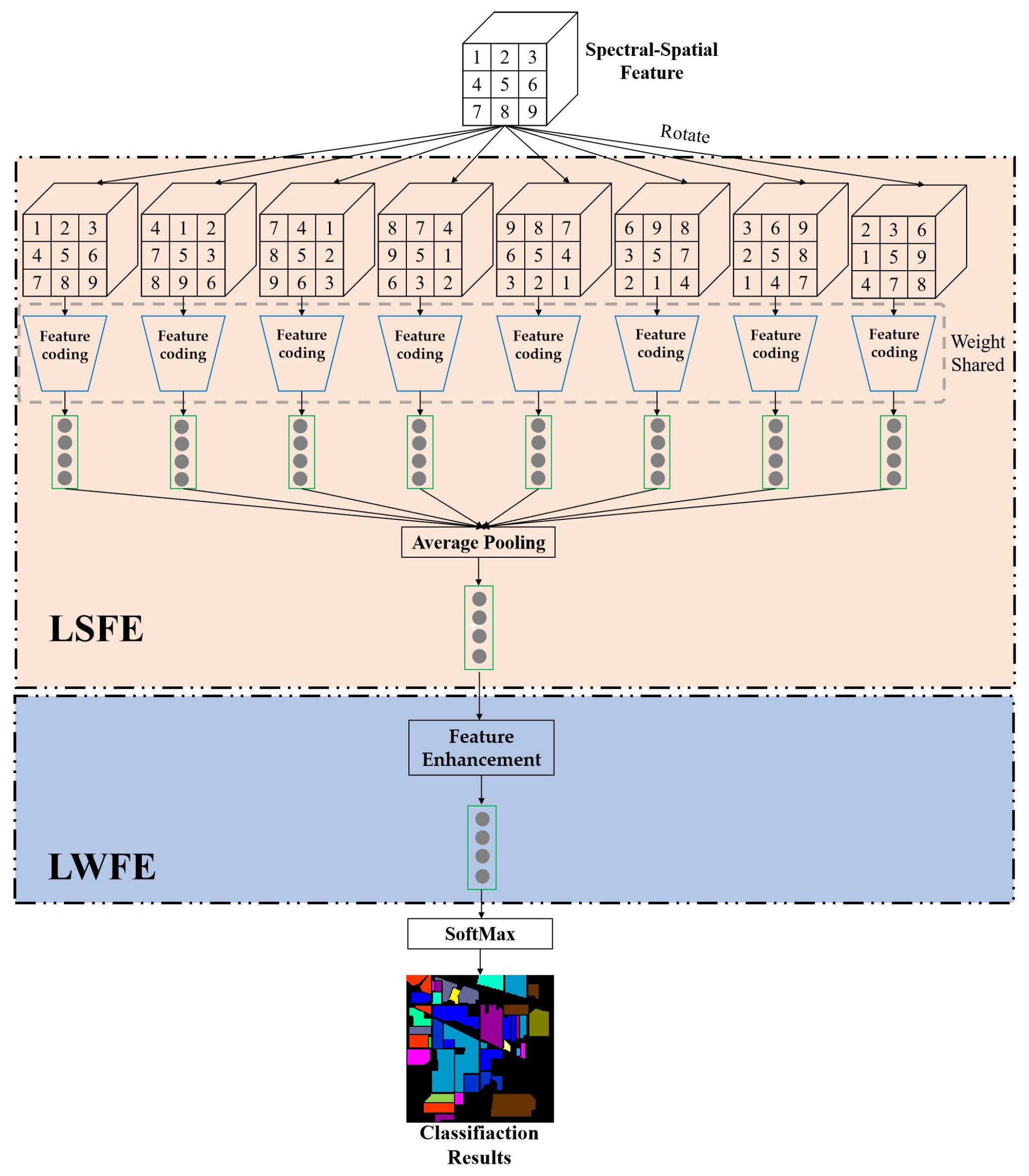
This paper proposes a simple and effective module named Local Spatial Feature Enhancement (LSFE) to solve the above problem. The LSFE module contains a rotate operator, a feature coding module, and an average pooling layer, as shown in Figure 5.

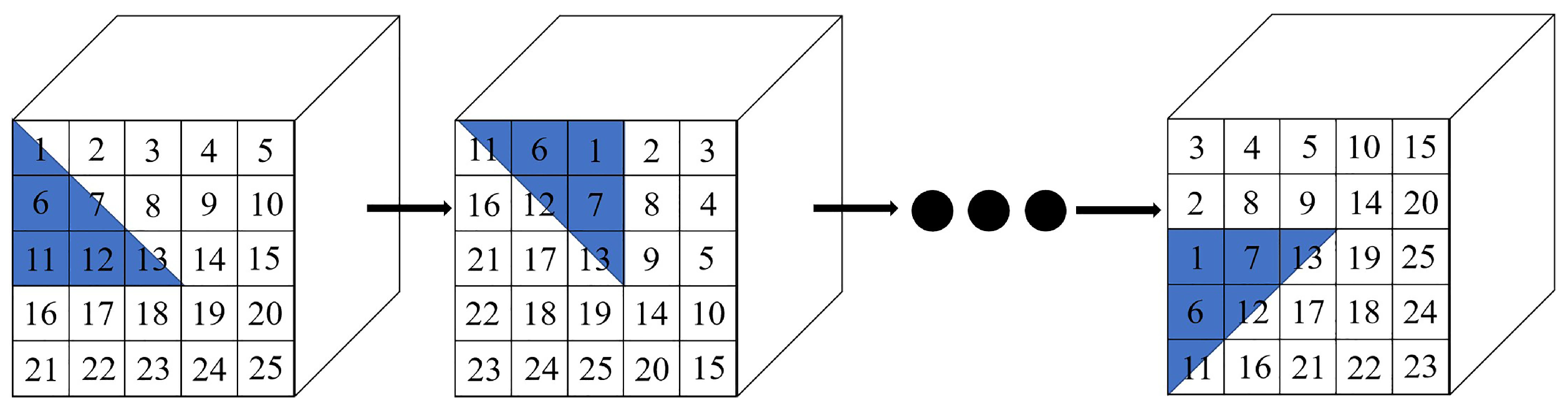
Specifically, each spatial-spectral feature is divided into eight non-overlapping regions using the center pixel as a reference. It also means that the center angle of each area is $2\pi /8$. Let ${\mathbf{I}}_{P\times P}^{S,\frac{i\left(2\pi \right)}{8}}$ denote the i-th region, where $i=(\left[\left.0,1,\dots ,7\right]\right)$. Then, each time, all regions are rotated $2\pi /8$ to produce a new spectral-spatial feature. It needs to rotate seven times to produce eight different spectral-spatial features.

Figure 6 shows an example. The blue area has a central pixel angle of $2\pi /8$. The radius of this area is $r=\lceil \mathrm{P}/2\rceil$. $\mathrm{P}$ represents the size of the spectral-spatial feature. $\lceil ·\rceil$ stands for rounding up. For instance, the size of the spatial-spectral feature is $5\times 5$. The radius of the rotation area is 3. After determining the region’s size, each rotation of $2\pi /8$ produces a new spatial-spectral feature. As shown in the second spatial-spectral feature in Figure 6, the blue region rotates to the corresponding position, and other regions rotate similarly. Therefore, the original spatial-spectral feature generates eight spatial-spectral features. This approach has the following benefits. (1) This approach is intuitive and straightforward to understand. (2) It can extract the position relationship between pixels without changing the shape of spatial-spectral features. (3) New spatial-spectral features can be directly fed into the network to extract features. (4) This module enhances the spatial features of the central pixel and improves the accuracy for the central pixel category.

After rotation, these spectral-spatial features are fed into a weight-shared feature coding module to obtain the corresponding spectral-spatial feature. The feature encoding network mainly includes two spatial attention layers and multi-layer feature extraction layers.

Table 4. The detailed structures of the local spatial feature enhancement (LSFE) module.

Layers	Input Size	Output Size	Kernel Size	S/P 1
Conv + ReLU	$P\times P\times N$	$P\times P\times 256$	$3\times 3\times 256$	1/1
SpaA 2	$P\times P\times 256$	$P\times P\times 256$	/	/
Conv + ReLU	$P\times P\times 256$	$P\times P\times 128$	$3\times 3\times 128$	1/1
SpaA	$P\times P\times 128$	$P\times P\times 128$	/	/
Conv + ReLU	$P\times P\times 128$	$P\times P\times 256$	$1\times 1\times 256$	/
Conv + ReLU	$P\times P\times 256$	$P\times P\times 512$	$3\times 3\times 512$	1/1
Conv + ReLU	$P\times P\times 512$	$P\times P\times 256$	$5\times 5\times 256$	1/1
Conv + ReLU	$K\times K\times 256$	$K\times K\times 128$	$3\times 3\times 128$	1/1
Conv + ReLU	$K\times K\times 128$	$K\times K\times 64$	$1\times 1\times 64$	/

¹ S/P represents Stride/Padding; ² SpaA represents Spatial-Attention.

lists the detailed structures of the feature encoding network.

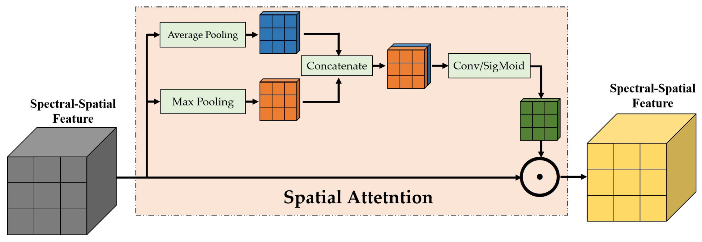
Each pixel surrounding the center pixel may have different effects on the center pixel. Thus, the weights of different pixels on the center pixel need to be recalibrated through the spatial attention mechanism. The spatial attention mechanism is shown in Figure 7. Different spectral curves represent different land-cover categories. Thus, spectral features can be used to change the pixel weights. The formula is as follows:

$${\mathbf{F}}^m=max\left(f\right(\mathbf{F}\left)\right)$$

(3)

$${\mathbf{F}}^a=average\left(f\right(\mathbf{F}\left)\right)$$

(4)

where ${\mathbf{F}}^m$ and ${\mathbf{F}}^a$ represent the features after max pooling and average pooling and $f\left(\mathbf{F}\right)$ is the spectral-spatial feature. Next, concatenate these features along the spectral dimension.

$${\mathbf{F}}^{\mathrm{c}}=concat\left[{\mathbf{F}}^{\mathrm{m}},{\mathbf{F}}^{\mathrm{a}}\right]$$

(5)

where ${\mathbf{F}}^{\mathrm{c}}$ is the feature after concatenation. Then, spatial attention can be calculated as follows:

$${\mathbf{F}}_{\mathrm{SpaA}}=\sigma \left(\mathrm{Conv}\left({\mathbf{F}}^{\mathrm{c}}\right)\right)\odot \left(f\mathbf{F}\right)$$

(6)

where ${\mathbf{F}}_{\mathrm{SpaA}}$ represents spectral-spatial features after spatial attention. Then, this feature is fed to multi-layer feature extraction layers. The output of the multi-layer feature extraction layers is ${\mathbf{F}}_v^i$:

$${\mathbf{F}}_v^i=\mathrm{FCM}\left({\mathbf{I}}_{P\times P}^{S,\frac{i\left(2\pi \right)}{8}}\right)$$

(7)

where $\mathrm{FCM}\left(·\right)$ denotes the weight-shared feature coding module, which includes two spatial attention layers and multi-layer feature extraction layers and ${\mathbf{F}}_v^i$ represents the output feature of the i-th branch. Finally, ${\mathbf{F}}_v^i$ is pooled into a feature vector, and the operation is defined with Equation (8):

$${\mathbf{F}}^{\mathrm{LSFE}}=\frac{1}{8}\sum _{0=1}^7{\mathbf{F}}_v^i$$

(8)

The output features of the LSFE module have the following functions. First, the output features extract the influence of surrounding pixels on the center pixel. Second, these features also contain the position relationship of each pixel and have rotation invariance.

2.4. Lightweight Feature Enhancement

A lightweight feature enhancement module (LWFE) is proposed to enhance the output features of the local spatial feature enhancement module. This module mainly focuses on enhancing important features, suppressing insignificance features, and improving classification accuracy.

The LWFE is shown in Figure 5. The output feature of the LSFE is fed to the LWFE module.

Table 5. The detailed structures of the lightweight feature enhancement (LWFE) module.

Layers	Input Size	Output Size	Kernel Size
Conv + ReLU	$K\times K\times 64$	$K\times K\times 256$	$1\times 1\times 256$
Conv + ReLU	$K\times K\times 256$	$K\times K\times 64$	$1\times 1\times 64$
AP	$K\times K\times 64$	$1\times 1\times 64$	/
FC	$1\times 1\times 64$	$1\times 16$	/

lists the datails of the LWFE module. Its formulation is defined with Equation (9):

$${\mathbf{F}}_{1\times 1}^{LWFE}=\mathrm{Ave}\left(\mathrm{ReLU}\left(\mathrm{Conv}\left(\mathrm{ReLU}\left(\mathrm{Conv}\left({\mathbf{F}}_{K\times K}^{LSFE}\right)\right)\right)\right)\right)$$

(9)

where $\mathrm{Ave}\left(·\right)$ denotes the average pooling; $\mathrm{Conv}\left(·\right)$ represents the 2D convolutional layer; $\mathrm{ReLU}\left(·\right)$ is the activate function, which is defined as $\mathrm{ReLU}\left(x\right)=\max \left(0,x\right)$; ${\mathbf{F}}_{K\times K}^{LSFE}$ denotes the output feature of the LSFE module, and $K\times K$ denotes the size of the feature; and ${\mathbf{F}}_{1\times 1}^{LWFE}$ represents the output feature of the LWFE module, which is also an enhanced feature.

The kernel size of all convolutional layers of LWFE is $1\times 1$. The reasons for using a convolution kernel of this size are as follows. (1) This convolution kernel can reduce the network parameters while enhancing the features. (2) It also maintains rotational invariance. Therefore, the whole LWFE module also retains rotation invariance. The output feature of the lightweight feature enhancement module is rotation invariant, while the LWFE module is also rotation invariant, so the whole network is also rotation invariant.

Finally, the enhanced feature is fed into a classifier to complete the classification.

$$C_p=\max \left(\frac{e^{{\mathbf{F}}_i}}{{\sum }_j^{16}{e}^{{\mathbf{F}}_j}}\right)$$

(10)

where $C_p$ is the predicted category. ${\mathbf{F}}_i$ and ${\mathbf{F}}_j$ are the i-th and j-th features of the feature vector of the LWFE module, respectively; that is, the category with the highest probability value is the prediction category of the network.

2.5. Loss Function

Due to the imbalance of samples, the feature of small samples may be lost during network training, which leads to the low classification accuracy of small samples. Therefore, this paper presents a dynamically weighted cross entropy loss according to the complexities of samples with different categories to improve the accuracy.

The proposed dynamical weighted cross entropy loss in m-th training epoch is defined as Equation (11):

$$\begin{array}{c}{J}^{\left(m\right)}\left(\left\{x^{\left(t\right)},y^{\left(t\right)}\right\}\left|\theta ,{\xi }^{\left(m,c\right)}\right.\right)\hfill \\ =-\frac{1}{T}{\displaystyle \sum _{t=1}^T}{\displaystyle \sum _{c=1}^C}{\xi }^{\left(m,c\right)}·\mathrm{I}\left\{y^{\left(t\right)}=c\right\}\log \frac{\exp \left({\theta }_c^T{x}^{\left(t\right)}\right)}{{\sum }_{k=1}^C\exp \left({\theta }_k^T{x}^{\left(t\right)}\right)}\hfill \end{array}$$

(11)

where $J^{\left(m\right)}$ represents the loss; $x^{\left(t\right)}$ and $y^{\left(t\right)}$ denote the t-th patch cube and corresponding category label; $\theta$ denotes the parameters of the softmax layer; T denotes the number of samples in a training batch; C denotes the number of categories of the dataset; $\mathrm{I}\left\{·\right\}$ denotes the indicator function, which equals one if the condition is satisfied and zero otherwise; and ${\xi }^{\left(m,c\right)}$ denotes the weight coefficient of the c-th category in the m-th training epoch, defined by Equation (12):

$${\xi }^{\left(m,c\right)}=\frac{{\sum }_{k=1}^C{A}^{\left(m-1,k\right)}}{C·A^{\left(m-1,c\right)}+\tau }$$

(12)

where $A^{(m,k)}$ denotes the validated accuracy of the k-th category in the m-th training epoch and $\tau$ is a small constant to avoid dividing by zero, which is set to ${10}^{-9}$ in this work.

The proposed SSARIN consists of the above three modules BS, LSFE, and LWFE. The corresponding loss functions are proposed according to the network characteristics. We introduce the experiments to demonstrate the proposed algorithm in the following.

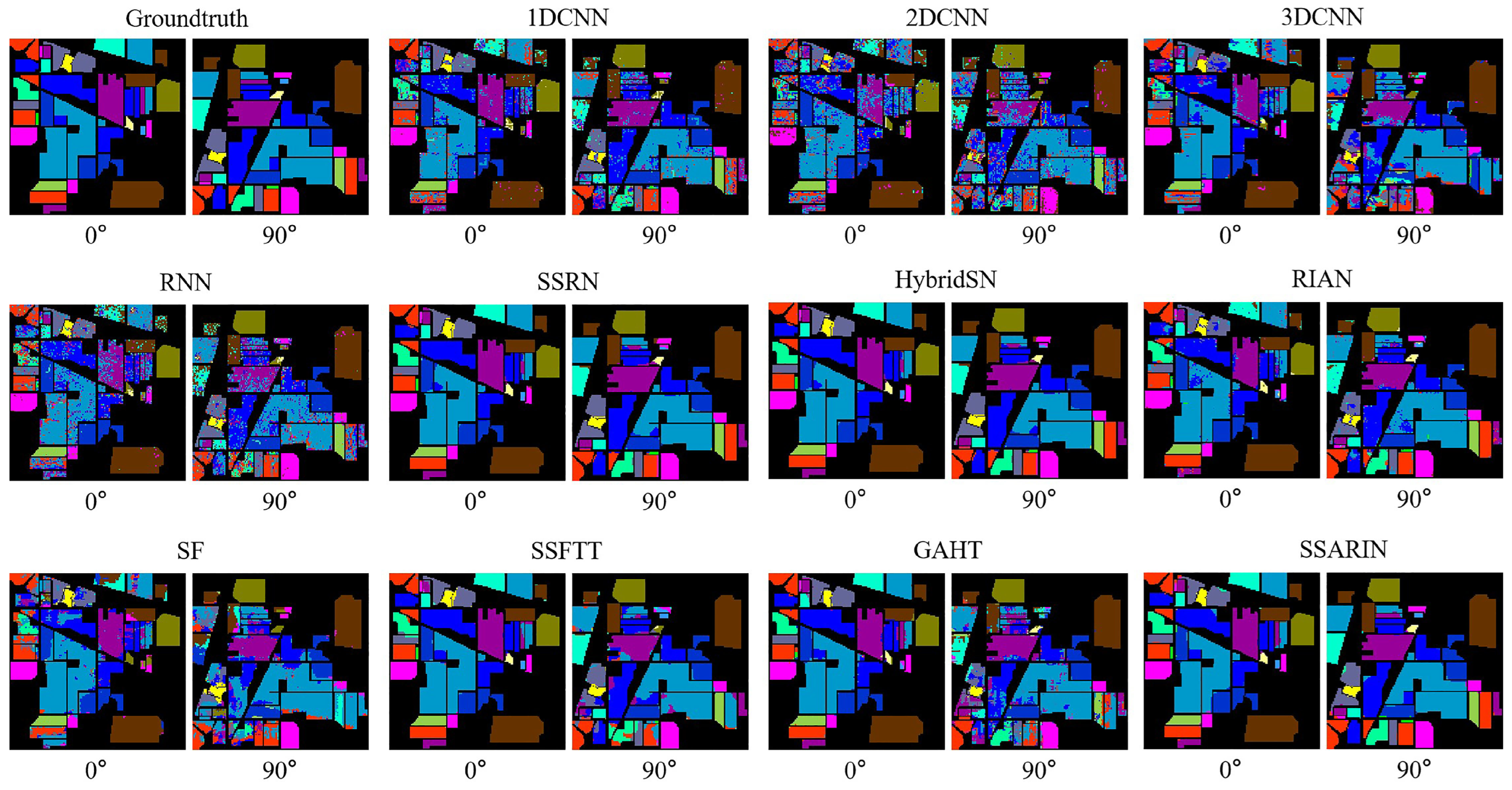
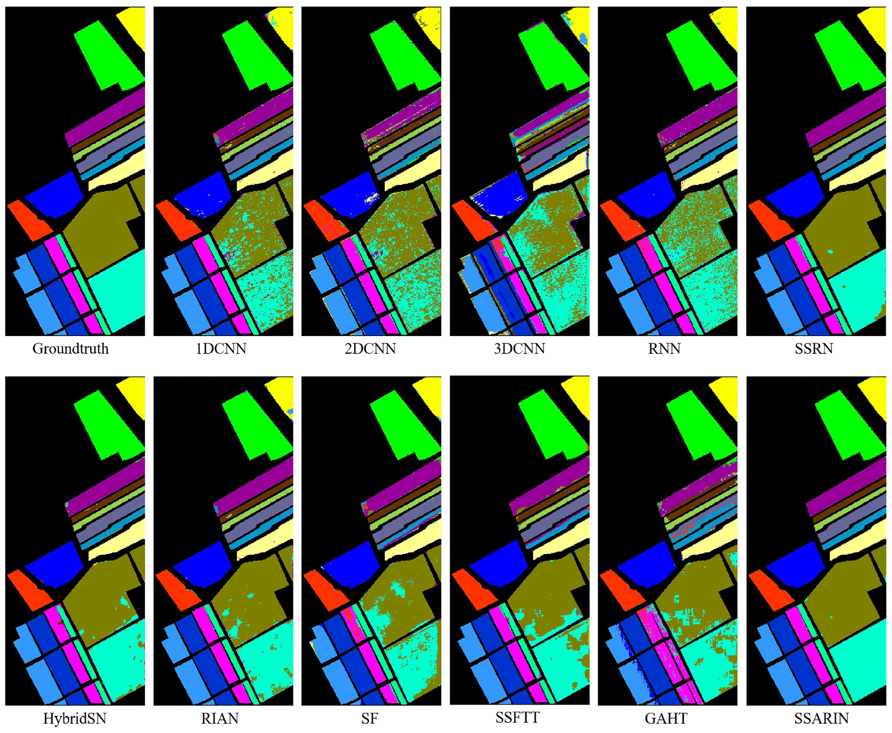
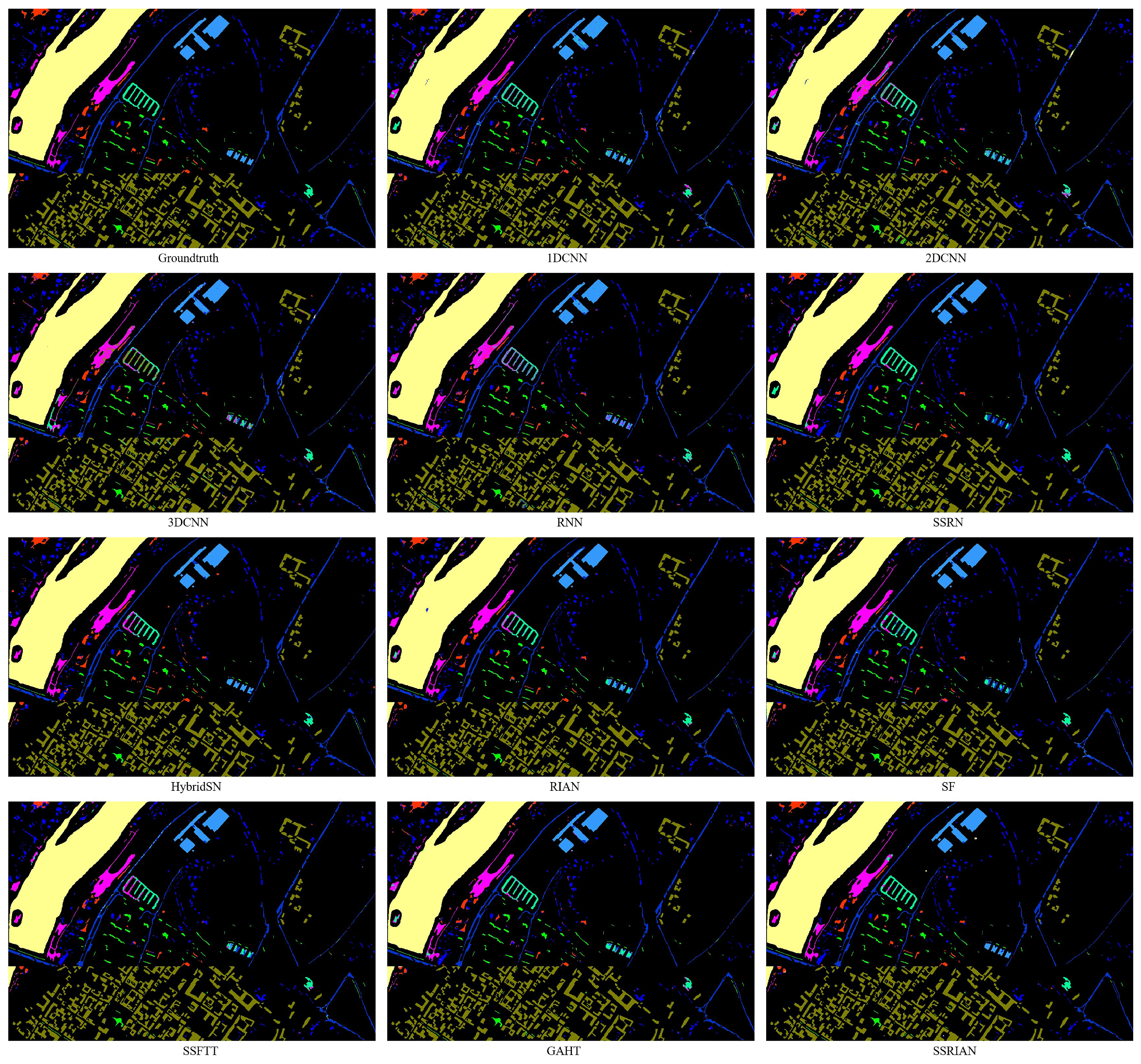
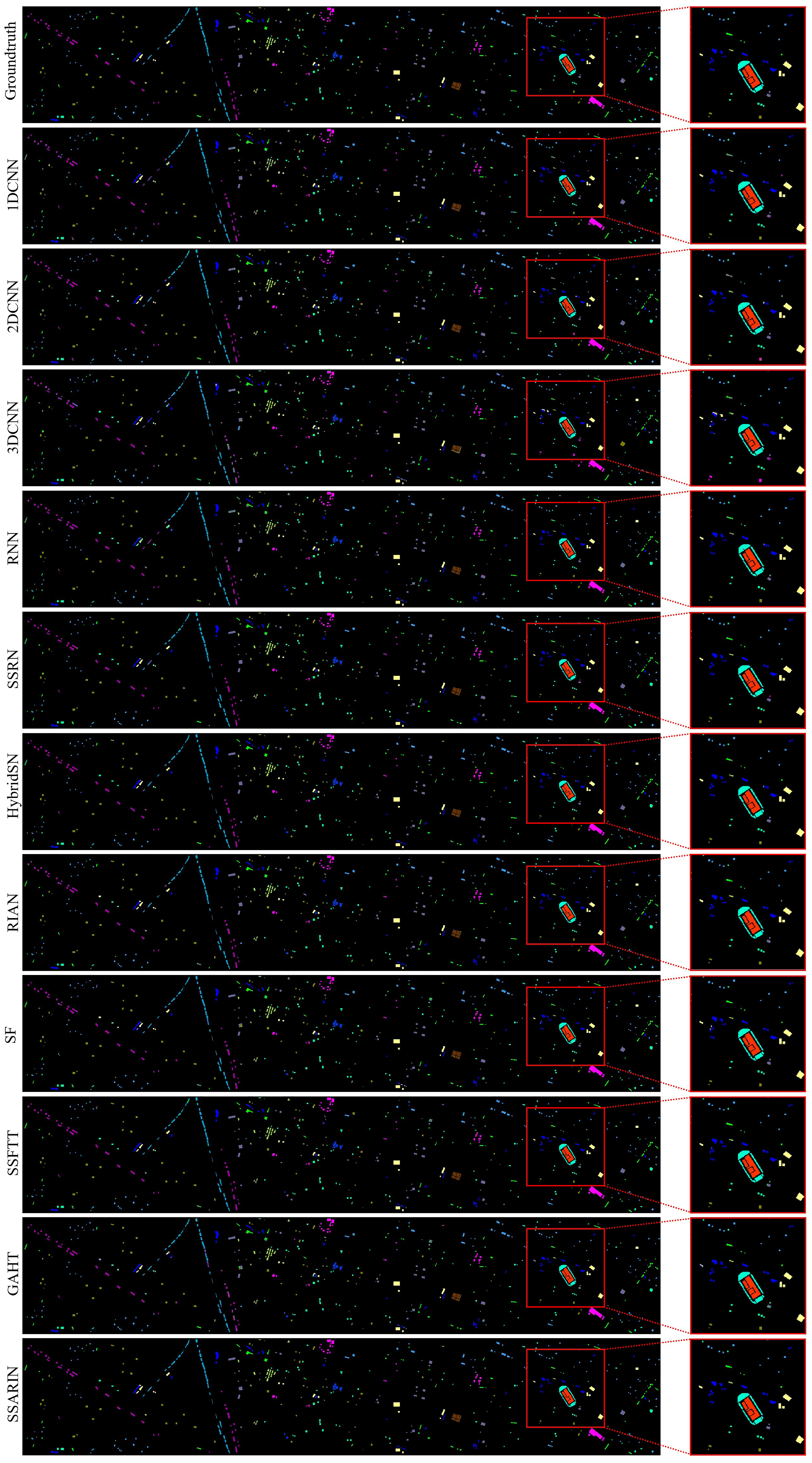
3. Results

In order to verify the performance of the different methods for HSI classification, extensive experiments have been carried out in this section. Section 3.1 introduces the dataset and evaluation metrics used in the experiment. Section 3.2 describes the compared methods and experiment design. Finally, the experimental results are drawn in Section 3.3.

3.1. Data Description and Evaluation Metrics

There are five public airborne hyperspectral image datasets (Indian Pines, Salinas, Pavia University, Pavia Center, and Houston) that were used to evaluate the methods.

3.1.1. Data Description

• Indian Pines (IP): As shown in Figure 8a, the IP dataset is composed of 145 × 145 pixels with 200 bands. Figure 8b shows the ground truth map of the IP dataset. This dataset has 16 different land-covers classes in the agriculture areas. It also includes 10,249 samples. The number of training and testing pixels is listed in

  Table 6. Training/testing samples of the Indian Pines (IP) dataset.

  Class No.	Class Name	Training	Testing
  1	Alfalfa	4	46
  2	Corn-Notill	142	1428
  3	Corn-Mintill	83	830
  4	Corn	23	237
  5	Grass-Pasture	48	483
  6	Grass-Trees	73	730
  7	Grass-Pasture-Mowed	2	28
  8	Hay-Windrowed	47	478
  9	Oats	2	20
  10	Soybean-Notill	97	972
  11	Soybean-Mintill	245	2455
  12	Soybean-Clean	59	593
  13	Wheat	20	205
  14	Woods	126	1265
  15	Buildings-Grass-Trees-Drives	38	386
  16	Stone-Steel-Towers	9	93
  Total	-	1018	10,249

  .

• Salinas (SA): Figure 9a shows the pseudo-color image of the SA dataset. It contains 512 × 217 pixels with 204 bands. Similar to the IP dataset, this dataset also has 16 categories and 54,129 samples in the agriculture areas, as shown in Figure 9b. In total, 2% of the pixels are randomly selected as training data. All samples are used as testing data.

  Table 7. Training/testing samples of the Salinas (SA) dataset.

  Class No.	Class Name	Training	Testing
  1	Brocoli-Green-Weeds-1	40	2009
  2	Brocoli-Green-Weeds-2	74	3726
  3	Fallow	39	1976
  4	Fallow-Rough-Plow	27	1394
  5	Fallow-Smooth	53	2678
  6	Stubble	79	3959
  7	Celery	71	3579
  8	Grapes-Untrained	225	11,271
  9	Soil-Vinyar-Develop	124	6203
  10	Corn-Senesced-Green-Weeds	65	3278
  11	Lettuce-Romaine-4wk	21	1068
  12	Lettuce-Romaine-5wk	38	1927
  13	Lettuce-Romaine-6wk	18	916
  14	Lettuce-Romaine-7wk	21	1070
  15	Vinyard-Untrained	145	7268
  16	Vinyard-Vertical-Trellis	36	1807
  Total	-	1076	54,129

  lists the class name and the number of training and testing samples.

• Pavia University (PU): The PU dataset includes 103 available spectral channels. The height and width of PU are 610 and 340. There are 42,776 samples from nine different land-cover categories in the PU database. Figure 10 shows the pseudo-color image and the ground truth classification map.

  Table 8. Training/testing samples of the Pavia University (PU) dataset.

  Class No.	Class Name	Training	Testing
  1	Asphalt	132	6631
  2	Meadows	372	18,649
  3	Gravel	41	2099
  4	Trees	61	3064
  5	Painte-Metal-Sheets	26	1345
  6	Bar-Soil	100	5029
  7	Bitumen	26	1330
  8	Self-Blocking-Bricks	73	3682
  9	Shadows	18	947
  Total	–	849	42,776

  lists the training and testing data of the PU dataset.

• Pavia Center (PC): The PC database comprises 1096 × 715 pixels with 102 available bands. Same as the PU dataset, it includes nine classes and 148,152 samples in the urban area. The pseudo-color image and the ground truth are shown in Figure 11. We randomly selected 0.5% of the data for each category as the training pixels. The entire dataset is the test set.

  Table 9. Training/testing samples of the Pavia Center (PC) dataset.

  Class No.	Class Name	Training	Testing
  1	Water	131	65,971
  2	Trees	15	7589
  3	Asphalt	6	3090
  4	Self-Blocking-Bricks	5	2685
  5	Bitumen	13	6584
  6	Tiles	18	9248
  7	Shadows	14	7287
  8	Meadows	85	42,826
  9	Bare-Soil	5	2863
  Total	–	292	148,152

  shows the number of testing and training samples.

• Houston: Houston is widely used as a benchmark database to evaluate the performance of HSI classification. It comprises 349 × 1905 pixels with 144 channels.

  Table 10. Training/testing samples of the Houston dataset.

  Class No.	Class Name	Training	Testing
  1	Grass-Healthy	125	1251
  2	Grass-Stressed	125	1254
  3	Grass-Synergic	69	697
  4	Tree	124	1244
  5	Soil	124	1242
  6	Water	32	325
  7	Residential	126	1268
  8	Commercial	124	1244
  9	Road	125	1252
  10	Highway	122	1227
  11	Railway	123	1235
  12	Parking-Lot-1	123	1233
  13	Parking-Lot-2	46	469
  14	Tennis-Court	42	428
  15	Running-Track	66	660
  Total	–	1496	15,029

  lists the number of training and testing data. There are 15 challenging land-cover classes and 15,029 samples. Similarly, the visualization of the image is given in Figure 12.

3.1.2. Evaluation Metrics

Three metrics were used to measure the performance of all algorithms. Let $\mathrm{M}\in {\mathbb{R}}^{\mathrm{n}\times \mathrm{n}}$ denote the confusion matrix and n represent the number of classes.

• Average Accuracy (AA) is the mean accuracy:

  $$\begin{array}{c}\hfill AA=\frac{{\sum }_{i=1}^n\frac{{\mathrm{M}}_{i,i}}{{\sum }_{j=1}^n{\mathrm{M}}_{i,j}}}{n}\end{array}$$

  (13)
• Overall Accuracy (OA) denotes the ratio of the number of correct samples to the total samples:

  $$\begin{array}{c}\hfill OA=\frac{{\sum }_{i=1}^n{\mathrm{M}}_{i,i}}{{\sum }_{i=1}^n{\sum }_{j=1}^n{\mathrm{M}}_{i,j}}\end{array}$$

  (14)
• Kappa coefficient ($\kappa$) is the consistency between forecast results and ground truth:

  $$\begin{array}{c}\hfill \kappa =\frac{\mathrm{OA}-p_e}{1-p_e}\end{array}$$

  (15)

  $$\begin{array}{c}\hfill p_e=\frac{{\sum }_{k=1}^n\left({\sum }_{i=1}^n{\mathrm{M}}_{i,k}·{\sum }_{j=1}^n{\mathrm{M}}_{k,j}\right)}{{\left({\sum }_{i=1}^n{\sum }_{j=1}^n{\mathrm{M}}_{i,j}\right)}^2}\end{array}$$

  (16)

  where ${\mathrm{M}}_{i,j}$ represents the i-th row and j-th column of the matrix $\mathrm{M}$; the value of ${\mathrm{M}}_{i,j}$ denotes the i-th category is classified as the j-th class; and ∑ stands for summation. Larger values represent better results.

3.2. Compared Methods and Experimental Design

This section briefly introduces the details of each compared method, mainly including the details and the experimental design.

3.2.1. Compared Methods

Several representatives and the most widely used deep learning algorithms are employed as compared methods. According to the different networks used, these methods are divided into CNN-based and transformer-based. CNN-based networks include 1D CNN [14], 2D CNN [60], 3D CNN [61], RNN [21], SSRN [27], HybridSN [31], and RIAN [13]. Transformer-based methods contain SF [45], SSFTT [46], and GAHT [47].

These algorithms are described as follows.

• 1D CNN [14]: This method uses two 1D convolutional layers to extract features.
• 2D CNN [60]: The spectral-spatial features are stacked to a 2D matrix. The matrix is considered as an image to feed into CNN.
• 3D CNN [61]: This method utilized the 3D convolutional layers to extract classification features.
• RNN [21]: The authors use RNN with the new activate function named parametric rectified tanh for HSI classification.
• SSRN [27]: A spectral-spatial residual network is proposed to classify hyperspectral samples.
• HybridSN [31]: This algorithm utilizes three layers of 3D CNN to extract spectral-spatial features. The output features are fed into a 2D CNN to classify hyperspectral pixels.
• RIAN [13]: The center spectral attention module recalibrates the spectral channels of image patches. The rectified spatial attention modules extract spectral-spatial features. A residual network connects these modules.
• SF [45]: A transformer-based backbone network.
• SSFTT [46]: A 3D and a 2D convolution layer are employed to extract spectral-spatial features. The output features are fed into a Gaussian-weighted tokenizer for feature transformation. Finally, an encoder module is utilized for feature learning to classify HSI samples.
• GAHT [47]: This work utilizes the hierarchical transformer network with the grouped pixel embedding module. This module confines the multi-head self-attention for extracting the spatial-spectral feature.

3.2.2. Experiment Design

Let $\mathrm{X}\in {\mathbb{R}}^{\mathrm{H}\times \mathrm{W}\times \mathrm{N}}$ be the original HSI, where $\mathrm{H}$ and $\mathrm{W}$ represent the height and width and $\mathrm{N}$ denotes the channel number. In the data preprocessing, all HSI datasets are normalized by:

$$\begin{array}{c}\hfill X^{\prime }=\frac{X-\min \left(X\right)}{\max \left(X\right)-\min \left(X\right)}\end{array}$$

(17)

where $\min \left(X\right)$ and $\max \left(X\right)$ represent the minimum and maximum value of the original HSI data $\mathbb{R}$.

In order to ensure the best performance of the compared algorithms, we introduce the following experimental designs. All the methods are implemented on Pytorch 1.12.1 with Python 3.9.13. The graphics processing unit (GPU) is an NVIDIA GeForce RTX 3090 with 24 GB memory, which was used to accelerate the experiments. The experiment designs are identical to the original literature and code, including the learning rate scheduler, the optimizer, and the HSI patches. In our methods, the initial learning rate of the learning rate scheduler is 0.001. It multiplies by 0.6 after every 10 epochs. The Adaptive Moment Estimation (Adam) optimizer with the default value is employed. Furthermore, a weight decay of 0.00005 is used to update the training parameters. The training and testing batch size of all methods is 64. The number of training epoch is 200.

Five airborne hyperspectral image datasets (IP, SA, PU, PC, and Houston) covering urban and agricultural regions are used to evaluate the algorithms. Different proportions are employed for each database. For the IP and Houston databases, 10% of samples are randomly selected as training data, and all samples are used for testing. For the SA and PU datasets, the train proportions are 2%. 0.5% of the samples for the PC database are selected for training. Table 6, Table 7, Table 8, Table 9 and Table 10 list the number of training and testing pixels of five datasets.

3.3. Experimental Results

We analyze the experimental results of the methods on the public datasets in detail, mainly including the patch size, the ablation experiment, and the performance of each algorithm in this section.

3.3.1. Size of HSI Patches

The size of the patch decides how much information is used for classification. Therefore, the patch size has a crucial impact on classification accuracy. The effects of different spatial sizes are first explored in this experiment. A series of patch sizes $\{7,9,11,13,15\}$ has been considered.

As shown in Figure 13, the accuracy does not always get better when the size increases. For IP and SA datasets, when the patch size is from 9 to 15, the accuracy of the proposed algorithm generally increases. The main reason is that the sample area is regular and dense, so as the local spatial information increases, it can provide more effective classification information. In other words, the IP and SA database has more significant smooth regions [47]. Thus, the patch size of the SA dataset is set to 15 × 15. Moreover, the IP dataset is set to 13 × 13. For PU, PC, and Houston datasets, the image of these databases has small and separate regions of land cover. Thus, the OAs of these datasets drop when the patch size exceeds the upper limit. The PC and Houston datasets’ patch size is 9 × 9. The spatial size of the PU dataset is set to 13 × 13.

3.3.2. Ablation Experiment

The proposed method consists of three parts (BS, LSFE, and LWFE). In order to verify the effect of each part, ablation experiments are conducted. Details of the experiments are as follows:

• Baseline network: This network only contains seven 2D convolution layers and one fully connected layer.
• Spectral-Spatial Attention (SSA) network: The spectral and spatial attention modules are added to the baseline network.
• Lightweight feature enhancement (LWFE) network: Based on the SSA network, the lightweight feature enhancement (LWFE) module is added to the network before the fully connected layer.
• SSARIN: Based on the LWFE network, a local spatial feature enhancement (LSFE) module is added to the network. This module is the key to ensuring rotation invariance.

Table 11. The OAs (%) of the ablation experiment on the public dataset.

Dataset	Baseline	SSA	LWFE	SSARIN
IP	98.15	98.36	98.53	98.59
SA	98.92	99.64	99.78	99.81
PU	97.73	98.91	99.03	99.05
PC	98.51	98.95	99.03	99.08
Houston	98.88	98.97	99.19	99.30

and

Table 12. OA (%) with different rotation angles for the ablation experiment on the public dataset.

Rotation	Network	IP	SA	PU	PC	Houston
0	LWFE	98.53	99.78	99.03	99.03	99.19
	SSARIN	98.59	99.81	99.05	99.08	99.30
90	LWFE	95.98	99.37	98.51	98.98	98.98
	SSARIN	98.59	99.81	99.05	99.08	99.30
180	LWFE	92.95	98.77	97.78	98.92	98.78
	SSARIN	98.59	99.81	99.05	99.08	99.30
270	LWFE	96.22	99.46	98.40	98.97	99.14
	SSARIN	98.59	99.81	99.05	99.08	99.30

show the results of the ablation experiment. As shown in Table 11, each module improves the classification OAs on different datasets. Compared to the baseline network, SSA improves the OAs by 0.21%, 0.72%, 1.15%, 0.44%, and 0.09%. It proves that the redundant bands do not provide adequate classification information. Sometimes, it reduces the accuracy of classification. It also illustrates that the weights of each channel are different for the spectral-spatial features. Thus, the BS module suppresses the redundant channels by recalibrating the weights of the different bands.

The OAs of the LWFE network are 0.17%, 0.14%, 0.12%, 0.08%, and 0.22% better than the SSA network. The LWFE module is primarily used to boost the output feature of the LSFE module to improve classification accuracy. The SSARIN network only promotes accuracy by 0.06%, 0.03%, 0.02%, 0.05%, and 0.11% compared to the LWFE network. However, the LSFE module added to the LWFE network can effectively maintain rotation invariance. Table 12 displays the OAs for different rotation degrees. It can be seen that when rotating at different degrees, the OAs of the LWFE network drop on all datasets, while the SSARIN remains stable. The ablation experiment indicates that the LSFE module improves the classification accuracy and retains the rotational invariance of the features. Therefore, the ablation experiment has demonstrated the role of each module and its impact on accuracy.

3.3.3. Performance of the Compared Methods

To evaluate the methods, the IP, SA, PU, PC, and Houston datasets are employed. The compared algorithms include 1D CNN [14], 2D CNN [60], 3D CNN [61], RNN [21], SSRN [27], HybridSN [31], RIAN [13], SF [45], SSFTT [46], and GAHT [47].

• Indian Pines: OAs of 1D CNN, 2D CNN, 3D CNN, RNN, SSRN, HybirdSN, RIAN, SF, SSFTT, GAHT, and RIRF at different rotation degrees are listed in

  Table 13. OA (%) with different rotation angles for the different methods on the IP dataset.

  Rotation	1D CNN	2D CNN	3D CNNN	RNN	SSRN	HybridSN	RIAN	SF	SSFTT	GAHT	SSARIN
  0	85.73	72.29	83.11	78.73	98.15	98.48	94.56	79.54	98.13	97.53	98.59
  90	85.73	66.79	66.46	78.73	97.05	91.19	94.56	64.30	86.88	79.50	98.59
  180	85.73	66.62	65.12	78.73	95.14	87.17	94.56	69.76	84.73	78.76	98.59
  270	85.73	65.84	67.05	78.73	96.97	91.30	94.56	63.99	85.81	80.08	98.59

  . When the rotation degree is 0, the performance of the spectral-spatial algorithms is better than the spectral methods. Meanwhile, the difference in OAs between the CNN-based classification model and the transformer-based model is insignificant. The OAs of 1D CNN, RNN, RIAN, and SSARIN at 0, 90, 180, and 270 degrees are 85.73%, 78.73%, 94.56%, and 98.59%. At the same time, these methods are both rotation invariant. 1D CNN, RNN, and RIAN are rotation invariant because these methods’ convolution kernel sizes are all 1 × 1. The 1 × 1 convolution is rotation invariant [13]. Among them, 1D CNN and RNN are based on spectral features and are not sensitive to spatial rotation. Thus, the above methods attain rotation invariance. In contrast, SSARIN is a method based on spatial-spectral features. SSARIN does not rely on 1 × 1 convolution to achieve rotation invariance. SSARIN obtains the position of the center pixel with the surrounding pixels through the LGFE module.
  The OAs of 2D CNN, 3D CNN, SSRN, HybridSN, SF, SSFTT, and GAHT significantly decrease at 90 degrees, 180 degrees, and 270 degrees. At a 90-degree rotation, the performance of these methods decreased by 5.5%, 16.65%, 1.1%, 7.29%, 15.24%, 11.25%, and 18.03%. The main reason is that these spectral-spatial convolutions ignore the position information between pixels. Therefore, the rotation causes the change of pixel position information, which leads to incorrect classification of the network.
  To further evaluate the compared algorithms, the accuracy in each class is listed in

  Table 14. Accuracy in each class, OA (%), AA (%), and $\kappa$ at 0 degrees on the IP dataset.

  Class No.	1D CNN	2D CNN	3D CNNN	RNN	SSRN	HybridSN	RIAN	SF	SSFTT	GAHT	SSARIN
  1	45.65	19.57	26.09	32.61	95.65	82.61	93.48	0.00	89.13	78.26	91.30
  2	82.00	60.57	76.54	72.76	96.22	98.11	92.37	72.97	99.58	96.85	98.25
  3	73.01	54.58	70.36	61.81	99.76	98.19	95.18	68.92	98.55	99.28	99.64
  4	72.15	41.35	52.32	48.10	99.16	98.73	91.98	56.54	91.56	97.89	99.58
  5	90.68	81.37	92.75	87.58	98.55	97.93	95.86	87.58	99.17	98.76	98.96
  6	95.58	97.81	94.75	97.81	95.34	99.73	99.45	87.67	98.36	97.53	97.53
  7	17.86	7.14	28.57	21.43	89.29	57.14	64.29	0.00	100.00	50.00	96.43
  8	98.74	94.56	100.00	100.00	100.00	100.00	99.16	100.00	100.00	100.00	100.00
  9	45.00	30.00	25.00	15.00	100.00	100.00	75.00	0.00	100.00	45.00	100.00
  10	85.18	59.88	75.31	67.70	96.30	98.05	87.96	73.15	95.06	97.74	98.46
  11	85.34	77.88	88.96	78.86	99.51	99.80	96.09	99.69	98.94	98.13	98.66
  12	88.70	43.68	67.12	78.25	94.10	98.65	86.17	54.30	91.74	98.15	94.44
  13	99.51	100.00	84.39	96.10	100.00	100.00	99.51	100.00	100.00	99.51	99.51
  14	95.18	93.75	96.68	94.94	100.00	99.37	98.74	93.91	99.68	98.58	99.84
  15	65.54	55.18	78.76	85.81	100.00	89.90	93.52	96.64	99.48	93.52	100.00
  16	83.87	64.52	68.82	87.10	96.77	100.00	92.47	88.17	95.70	83.87	95.70
  AA	76.56	61.36	70.37	68.68	97.54	94.89	91.33	63.28	97.31	89.57	98.02
  OA	85.73	72.29	83.11	78.73	98.15	98.48	94.56	79.54	98.13	97.53	98.59
  Kappa	83.71	68.11	80.61	75.65	97.88	98.26	93.78	76.45	97.86	97.18	98.39

  and

  Table 15. Accuracy in each class, OA (%), AA (%), and $\kappa$ at 90 degrees on the IP dataset.

  Class No.	1D CNN	2D CNN	3D CNNN	RNN	SSRN	HybridSN	RIAN	SF	SSFTT	GAHT	SSARIN
  1	45.65	2.17	0.00	32.61	80.43	78.26	93.48	0.00	15.22	71.74	91.30
  2	82.00	55.05	57.56	72.76	95.66	92.79	92.37	49.23	91.81	64.85	98.25
  3	73.01	42.41	28.43	61.81	96.87	86.99	95.18	43.49	50.24	52.65	99.64
  4	72.15	37.97	30.38	48.10	97.47	79.32	91.98	24.47	74.26	79.75	99.58
  5	90.68	70.19	66.87	87.58	92.96	87.16	95.86	82.40	88.82	77.43	98.96
  6	95.58	96.85	81.23	97.81	96.30	99.73	99.45	85.62	97.81	96.85	97.53
  7	17.86	0.00	0.00	21.43	42.86	14.29	64.29	0.00	35.71	100.00	96.43
  8	98.74	93.31	99.79	100.00	100.00	100.00	99.16	100.00	100.00	100.00	100.00
  9	45.00	0.00	0.00	15.00	75.00	10.00	75.00	0.00	30.00	0.00	100.00
  10	85.18	50.93	59.16	67.70	96.30	98.05	87.96	73.15	95.06	97.74	98.46
  11	85.34	75.52	81.38	78.86	96.19	84.36	87.96	60.70	76.54	96.73	98.66
  12	88.70	26.48	40.64	78.25	96.29	83.14	86.17	28.33	75.04	55.14	94.44
  13	99.51	84.39	0.00	96.10	100.00	100.00	99.51	0.00	99.51	62.93	99.51
  14	95.18	93.99	94.70	94.94	99.84	98.42	98.74	90.67	98.50	95.81	99.84
  15	65.54	54.66	54.15	85.81	94.56	80.57	93.52	9.84	96.89	66.32	100.00
  16	83.87	48.39	72.04	87.10	98.92	100.00	92.47	91.40	93.55	72.04	95.70
  AA	76.56	52.02	47.90	68.68	91.37	80.48	91.33	46.57	79.96	69.12	98.02
  OA	85.73	66.79	66.46	78.73	97.05	91.19	94.56	64.30	86.88	79.50	98.59
  Kappa	83.71	61.72	61.21	75.65	96.64	89.94	93.78	58.48	84.96	76.43	98.39

  . At 0 degrees, the proposed SSARIN achieves state-of-the-art compared with other methods. It significantly improves the OAs of the “Corn”, “Hay-Windrowed”, “Oats”, “Soybean-Notill”, and “Buildings-Grass-Trees-Drives”, classes. At 90 degrees, it not only maintains the best OAs in the above categories, but also achieves the best OAs in the “Corn-Notill”, “Corn-Mintill”, “Grass-Pasture”, “Soybean-Mintill”, and “Woods” categories. For instance, the SSRN achieves the best accuracy in seven classes without rotation. It only attains the best performance of the four categories after rotating 90 degrees.
  Figure 14 shows the classification maps on the IP dataset. It intuitively displays the performance of each method. When the image is rotated, the edge information of the HSI patch changes. Therefore, the compared methods that do not sufficiently extract the spatial edge position information have a drop in test accuracy. The sufficient learning of spatial edge position information shows that the proposed SSARIN has superior classification results and is invariant to the rotation.

2.

Salinas:

Table 16. OA (%) with different rotation angles for the different methods on SA dataset.

Rotation	1D CNN	2D CNN	3D CNNN	RNN	SSRN	HybridSN	RIAN	SF	SSFTT	GAHT	SSARIN
0	91.61	89.72	88.73	88.83	99.67	99.65	97.13	96.27	99.36	98.46	99.81
90	91.61	87.02	79.42	88.83	99.19	99.05	97.13	89.57	94.77	89.79	99.81
180	91.61	86.79	77.41	88.83	99.09	97.85	97.13	90.93	93.12	87.68	99.81
270	91.61	86.88	78.68	88.83	99.45	99.11	97.13	87.37	93.32	88.06	99.81

reports the performance of these methods at different rotation degrees. Similar to the IP dataset, the OAs of 1D CNN, RNN, RIAN, and SSARIN as different angles are 91.61%, 88.83%, 97.13%, and 99.81%, respectively. The performance of SSARIN is better than other networks in terms of OA. When the angles are 90, 180, and 270, the OAs of 2D CNN, 3D CNN, SSRN, HybridSN, SF, SSFTT, and GAHT significantly decrease. At a rotation degree of 180, the performance of these methods decreased by 2.93%, 11.32%, 0.58%, 1.8%, 5.34%, 6.24%, and 10.78%. It is a smaller drop compared to the IP dataset. The reason is that the sample area of the SA dataset is more regular and smooth than the IP dataset. According to the experiment, the transformer-based method is more sensitive to rotation invariance than the CNN-based method. The reason is that the CNN-based convolutional layer focuses on local information, while the transformer-based approach focuses more on global information. Rotation changes the local information of HSI, resulting in the performance of the transformer-based method being worse than the CNN-based method.

To further evaluate the compared algorithms, the accuracy in each category at 180 degrees is listed in

Table 17. Accuracy in each class, OA (%), AA (%), and $\kappa$ at 180 degrees on the SA dataset.

Class No.	1D CNN	2D CNN	3D CNNN	RNN	SSRN	HybridSN	RIAN	SF	SSFTT	GAHT	SSARIN
1	99.50	98.36	90.84	99.30	100.00	100.00	99.70	99.90	100.00	98.71	100.00
2	99.06	96.46	92.27	99.97	100.00	99.68	99.81	99.62	100.00	99.95	100.00
3	99.24	95.55	95.14	98.28	100.00	100.00	99.04	99.44	100.00	99.34	100.00
4	97.70	95.55	80.42	99.35	100.00	93.54	99.28	99.71	96.77	18.44	99.86
5	98.84	90.03	90.72	94.47	96.27	96.45	98.81	83.53	93.99	88.87	99.14
6	99.75	97.47	81.66	99.85	100.00	99.95	100.00	100.00	100.00	99.90	99.97
7	99.55	96.54	94.86	99.61	100.00	99.80	100.00	95.64	99.86	85.00	100.00
8	82.71	81.45	68.00	65.68	99.48	96.72	94.45	84.77	87.57	87.98	99.42
9	99.79	99.45	97.02	99.82	100.00	100.00	99.11	99.85	99.50	99.92	100.00
10	92.13	79.56	54.85	94.94	99.60	97.56	97.62	92.28	92.71	79.99	99.91
11	95.51	75.09	86.24	91.29	100.00	91.48	95.69	68.26	72.65	76.59	99.81
12	99.69	99.58	86.20	99.95	99.64	99.58	99.64	98.75	98.18	51.69	100.00
13	97.60	90.61	1.75	99.56	92.69	99.78	99.02	97.27	86.35	96.94	99.24
14	92.80	88.32	62.80	95.33	99.44	94.86	97.76	99.16	98.69	91.87	100.00
15	73.78	60.83	76.49	78.10	96.73	95.28	92.43	74.26	81.18	81.59	100.00
16	93.85	88.05	79.25	98.01	99.89	99.61	95.30	98.12	99.61	99.94	100.00
AA	95.09	89.56	74.91	94.59	98.98	97.77	97.98	93.16	94.19	84.79	99.83
OA	91.61	86.79	77.41	88.83	99.09	97.85	97.13	90.93	93.12	87.68	99.81
Kappa	90.66	85.27	74.80	87.61	98.99	97.61	96.80	89.90	92.34	86.28	99.79

. At 180 degrees, SSARIN maintains the best OAs in 11 classes. Figure 15 shows the classification maps on the SA dataset. The performance of each method is represented intuitively. The compared methods are weak in the performance of the “Vinyard-Untrained” and “Grapes-Untrained” classes. At the same time, the proposed algorithm has superior performance in the above categories. Moreover, the classification map of the SSARIN is also smooth.

3.

Pavia University:

Table 18. OA (%) with different rotation angles for the different methods on the PU dataset.

Rotation	1D CNN	2D CNN	3D CNNN	RNN	SSRN	HybridSN	RIAN	SF	SSFTT	GAHT	SSARIN
0	89.64	93.00	85.28	88.83	99.38	98.97	98.05	95.38	98.83	98.00	99.05
90	89.64	88.53	74.93	88.83	98.73	97.51	98.05	85.04	95.83	90.06	99.05
180	89.64	85.69	74.53	88.83	97.79	95.55	98.05	87.50	93.70	87.99	99.05
270	89.64	89.67	74.09	88.83	98.38	97.35	98.05	86.02	94.12	92.40	99.05

lists the OAs of all methods at various rotation angles. 1D CNN, RNN, and SSARIN achieve rotation invariance because these methods’ convolution kernel sizes are all 1 × 1. The OAs of these methods at 0, 90, 180, and 270 degrees are 89.64%, 88.83%, and 98.05%. The performance of the SSARIN is 99.05%. When the rotation degree is 0, the performance of SSARIN is second only to that of SSRN. When the rotation degrees change, the OAs of 2D CNN, 3D CNN, SSRN, HybridSN, SF, SSFTT, and GAHT drop significantly. At a rotation degree of 270, the performance of these methods decreased by 3.33%, 11.19%, 1%, 1.58%, 9.36%, 4.71%, and 5.6%.

To further evaluate the compared algorithms, the quantitative indicators at the rotation of 270 degrees are shown in

Table 19. Accuracy in each class, OA (%), AA (%), and $\kappa$ at 270 degrees on the PU dataset.

Class No.	1D CNN	2D CNN	3D CNNN	RNN	SSRN	HybridSN	RIAN	SF	SSFTT	GAHT	SSARIN
1	90.68	87.86	86.93	86.31	98.40	99.16	98.46	85.46	90.27	94.92	100.00
2	95.66	97.61	90.67	95.79	99.74	99.92	99.40	94.21	99.7	99.27	99.80
3	64.46	74.27	25.82	73.03	99.09	82.71	88.76	72.75	92.09	64.89	97.38
4	85.70	79.18	71.41	88.90	93.05	92.89	96.83	86.59	95.04	83.09	96.67
5	99.70	99.63	13.46	99.48	99.85	100.00	99.78	99.70	98.66	97.84	99.93
6	76.85	84.21	65.48	80.97	100.00	99.03	98.67	94.97	99.68	97.65	100.00
7	84.89	79.17	43.53	72.18	100.00	98.95	97.82	62.71	79.62	91.88	99.62
8	87.75	76.56	57.77	77.24	93.54	89.38	95.06	74.45	68.25	69.42	95.82
9	99.89	94.51	11.72	99.26	97.71	97.57	99.89	72.23	95.99	85.22	94.40
AA	87.29	85.89	51.87	85.91	97.39	95.49	97.14	79.56	91.04	97.13	98.18
OA	89.64	89.67	74.09	88.83	98.38	97.35	98.05	86.02	94.12	92.40	99.05
Kappa	86.16	86.19	65.36	85.15	97.85	96.49	97.42	81.62	92.22	89.90	98.74

. SSARIN maintains the best OAs in four classes. Meanwhile, it has the best performance of the OA, AA, and Kappa. Figure 16 shows the performance of each method intuitively. Furthermore, the classification map of SSARIN is smooth.

4.

Pavia Center:

Table 20. OA (%) with different rotation angles for the different methods on the PC dataset.

Rotation	1D CNN	2D CNN	3D CNNN	RNN	SSRN	HybridSN	RIAN	SF	SSFTT	GAHT	SSARIN
0	97.44	97.34	97.22	97.34	98.43	98.63	98.35	98.25	98.35	98.61	99.08
90	97.44	96.46	95.43	97.34	98.30	98.58	98.35	97.17	97.17	97.75	99.08
180	97.44	96.93	96.00	97.34	98.34	98.30	98.35	97.33	96.97	97.61	99.08
270	97.44	96.39	96.29	97.34	98.40	98.51	98.35	97.33	97.15	97.34	99.08

lists the OAs of all the algorithms at different rotation degrees. The OAs of 1D CNN, RNN, RIAN, and SSARIN at 0, 90, 180, and 270 degrees are 97.44%, 97.34%, 98.35%, and 98.05%. The above methods are both rotation invariant. When the rotation degree is 0, the performance of SSARIN has the best performance. When the rotation degrees change, the OAs of 2D CNN, 3D CNN, SSRN, HybridSN, SF, SSFTT, and GAHT drop significantly. At a rotation degree of 90, the performance of these methods decreased by 0.88%, 1.79%, 0.13%, 0.05%, 1.08%, 1.18%, and 0.86%. Compared to the IP, SA, and PU datasets, these algorithms do not have much accuracy degradation on the PC dataset. Our analysis is due to the small number of categories in the PC dataset and the concentration of sample areas.

To further evaluate the compared algorithms, the metrics at 90 degrees are shown in

Table 21. Accuracy in each class, OA (%), AA (%), and $\kappa$ at 90 degrees on the PC dataset.

Class No.	1D CNN	2D CNN	3D CNNN	RNN	SSRN	HybridSN	RIAN	SF	SSFTT	GAHT	SSARIN
1	99.96	99.76	99.98	99.99	99.99	99.99	99.90	99.83	99.96	99.98	100.00
2	94.81	96.43	96.46	91.73	98.67	92.25	94.67	96.33	96.25	90.00	96.37
3	81.03	69.19	82.88	90.97	83.69	90.74	90.55	77.12	69.19	75.76	91.26
4	75.61	73.74	53.07	57.28	97.58	75.90	78.44	81.82	72.03	92.74	95.38
5	89.87	81.12	83.25	98.34	91.83	98.12	96.69	93.77	93.41	92.27	97.28
6	93.46	92.52	92.54	98.71	99.91	99.42	99.28	92.63	94.87	99.37	99.76
7	92.18	91.03	82.85	92.19	84.66	96.12	92.19	88.71	88.45	88.34	97.86
8	99.35	98.73	99.26	98.58	99.94	99.84	99.83	99.83	99.14	99.89	99.59
9	99.72	95.28	97.42	99.93	99.51	94.48	93.89	86.57	97.07	93.99	94.24
AA	91.78	88.64	87.52	91.00	95.09	94.10	93.94	90.74	90.04	92.48	96.86
OA	97.44	96.39	96.29	97.34	98.40	98.51	98.35	97.33	97.15	97.34	99.08
Kappa	96.38	94.88	94.72	96.24	97.73	97.89	97.66	96.22	95.97	96.79	98.69

. SSARIN maintains the best performance of the OA, AA, and Kappa. At the same time, the performance of each method is represented intuitively in Figure 17.

5.

Houston: OAs of 1D CNN, 2D CNN, 3D CNN, RNN, SSRN, HybirdSN, RIAN, SF, SSFTT, GAHT, and SSARIN at different rotation degrees are listed in

Table 22. OA (%) with different rotation angles for the different methods on the Houston dataset.

Rotation	1D CNN	2D CNN	3D CNNN	RNN	SSRN	HybridSN	RIAN	SF	SSFTT	GAHT	SSARIN
0	91.96	95.22	90.45	91.90	99.23	98.81	97.33	96.75	98.53	97.78	99.30
90	91.96	93.21	77.12	91.90	97.91	98.35	97.33	86.97	91.96	89.13	99.30
180	91.96	83.74	83.58	91.90	98.47	98.17	97.33	93.97	96.05	94.58	99.30
270	91.96	93.61	76.23	91.90	97.99	97.87	97.33	87.42	90.50	88.85	99.30

. The OAs of 1D CNN, RNN, RIAN, and SSARIN are 91.96%, 91.90%, 97.33%, and 99.30%. At a rotation degree of 180, the performance of these methods decreased by 11.48%, 6.87%, 0.76%, 0.64%, 2.78%, 1.48%, and 3.2%. To further evaluate the compared algorithms, the OA, AA, and Kappa at 180 degrees are shown in

Table 23. Accuracy in each class, OA(%), AA(%), and $\kappa$ at 180 degrees on the Houston dataset.

Class No.	1D CNN	2D CNN	3D CNNN	RNN	SSRN	HybridSN	RIAN	SF	SSFTT	GAHT	SSARIN
1	97.04	100.00	94.16	90.73	98.96	97.92	99.04	96.40	98.32	92.25	100.00
2	99.36	98.25	90.99	97.77	99.28	99.36	98.41	97.69	98.64	98.48	98.88
3	98.85	97.85	96.56	100.00	100.00	99.86	100.00	99.86	100.00	99.86	100.00
4	98.79	95.82	95.66	98.71	99.68	99.76	97.51	93.49	99.28	95.50	99.84
5	98.63	99.68	97.58	99.19	100.00	100.00	99.76	99.76	100.00	99.60	100
6	98.77	92.31	82.15	99.69	98.15	99.69	95.38	93.54	97.23	96.62	98.15
7	86.51	87.54	74.53	87.38	99.53	96.29	97.87	90.14	87.38	96.29	98.82
8	85.29	87.14	64.79	92.36	97.11	98.31	97.51	90.35	89.95	92.52	100.00
9	77.32	83.15	88.66	76.36	94.65	92.01	92.01	88.50	92.33	92.65	96.25
10	92.99	97.64	72.78	95.27	99.35	99.35	96.09	97.23	99.51	93.56	100.00
11	88.58	93.12	71.17	85.91	97.09	97.98	96.19	92.15	96.68	88.91	99.51
12	95.30	95.38	72.69	89.53	98.86	98.62	98.38	89.05	94.08	87.75	98.95
13	59.91	81.45	79.74	72.92	94.03	96.59	92.54	88.06	92.54	94.88	99.58
14	98.13	96.96	81.78	100.00	100.00	100.00	97.43	98.36	100.00	99.77	100.00
15	99.85	96.62	98.03	98.94	99.55	99.70	99.70	98.79	99.85	99.85	100.00
AA	91.69	93.52	84.08	92.32	98.42	98.36	97.19	94.22	96.39	95.23	99.33
OA	91.96	83.74	83.58	91.90	98.47	98.17	97.33	93.97	96.05	94.58	99.30
Kappa	91.30	93.23	82.24	91.25	98.35	98.02	97.11	93.48	95.73	94.15	99.24

. SSARIN maintains the best OAs in 12 classes. Meanwhile, it has the best performance of the OA, AA, and Kappa. Through Figure 18, it is very intuitive to conclude that the classification map of SSARIN is smoother than other compared methods.

4. Discussion

Figure 14, Figure 15, Figure 16, Figure 17 and Figure 18 illustrate the classification maps of different methods on five datasets. Table 13, Table 14, Table 15, Table 16, Table 17, Table 18, Table 19, Table 20, Table 21, Table 22 and Table 23 detail the class accuracy, AA, OA, and kappa coefficient for these algorithms on corresponding datasets. Our algorithm not only delivers superior results, but also maintains consistent overall accuracy at varying rotation angles. Building upon this analysis, we explore the time efficiency of the models.

Table 24. The training and testing time of the different methods.

Dataset	Time (s)	1D CNN	2D CNN	3D CNN	RNN	SSRN	HybridSN	RIAN	SF	SSFTT	GAHT	SSARIN
IP	Training	16.53	194.61	15.11	26.62	70.08	47.03	51.31	105.70	55.90	125.17	594.51
	Testing	0.19	0.69	0.22	0.21	0.67	0.29	0.40	1.42	0.41	0.82	6.59
SA	Training	18.01	162.33	17.20	28.63	81.99	44.50	49.99	110.16	59.50	129.16	674.84
	Testing	0.68	2.09	1.12	1.08	3.52	1.76	2.06	7.96	1.97	5.29	27.61
PU	Training	16.47	60.69	15.14	18.51	56.08	34.95	42.03	81.31	56.07	104.51	563.91
	Testing	0.46	1.05	0.62	0.80	1.91	1.41	1.61	6.19	1.58	4.08	24.617
PC	Training	14.62	29.63	11.13	15.76	45.93	33.23	35.54	85.75	41.44	92.54	510.75
	Testing	0.79	3.36	2.07	2.72	5.54	3.88	5.53	5.01	5.30	11.72	66.78
Houston	Training	20.33	87.89	26.70	34.65	95.62	37.62	76.89	156.66	83.28	165.53	976.77
	Testing	0.24	0.63	0.26	0.30	0.75	0.41	0.72	1.94	0.54	1.18	7.88

outlines the training and testing time for each algorithm. Notably, 3D CNN consistently exhibits the fastest training times across all datasets. 1D CNN emerges as the model with the fastest testing times for each dataset, indicating that it performs well in terms of time efficiency during the testing phase. In contrast, SSARIN displays the longest training and testing times. There are two main reasons for this. (1) The network contains eight branches, resulting in a more complex structure. (2) When rotating the features, it is necessary to load the features from the GPU to the CPU for rotation and then reload the rotated features from the CPU back to the GPU.

Table 25. The parameters of the different methods.

Method	1D CNN	2D CNN	3D CNNN	RNN	SSRN	HybridSN	RIAN	SF	SSFTT	GAHT	SSARIN
Parameters	74,196	109,613,786	115,564	235,024	129,068	108,912	89,260	99,640	950,280	1,228,940	41,694,672

enumerates the parameters for each method. SSARIN possesses a relatively high parameter count (41,694,672), making it the second most complex model in this list. The main reason is that the network contains eight branches, and the structure of each branch is the same. Therefore, the network requires a larger number of parameters. This complexity is a factor in its longer training and testing times, as observed in the previous analysis.

1D CNN has the fewest parameters (74,196), indicating that it is the simplest model in terms of architecture. This simplicity contributes to the model’s previously observed fast testing times, as there are fewer parameters to compute during the testing phase. However, the trade-off is a limited capacity to capture complex patterns in the data, which impacts performance in classification. 2D CNN has the highest number of parameters (109,613,786), indicating that this model has the most complex architecture among the models listed. The main reason is that it uses multiple fully connected layers, and the fully connected layers contain many network nodes. This intricacy results in heightened computational demands during training and testing and increased processing times.

The parameter numbers and training time for other algorithms do not differ significantly. This section discusses the classification performance of various algorithms on different datasets. Although the proposed SSARIN requires more parameters and computation time, it is within a reasonable and acceptable range.

5. Conclusions

This paper proposes a spectral-spatial attention rotation-invariant classification network for the airborne hyperspectral image. The SSARIN is specifically designed to explore rotation-invariant features for hyperspectral classification. It mainly contains a band selection module, a local spatial feature enhancement module, and a lightweight feature enhancement module.

In the data pre-processing stage, using PCA to reduce the spectral dimensions can effectively reduce the network parameters and training time. However, PCA is not mandatory. After pre-processing, the HSI patch is fed into the band selection module for feature extraction. The band selection (BS) module achieves redundant band suppression by recalibrating the weights of each band. Furthermore, a local spatial feature enhancement (LSFE) module is introduced to extract spectral-spatial features while maintaining rotational invariance. The LSFE module not only extracts spatial-spectral features but also records position information to maintain rotational invariance, providing a robust solution for hyperspectral classification. The proposed method is capable of extracting rotation-invariant spectral-spatial features without requiring additional parameters or constraints. Finally, a lightweight feature enhancement (LWFE) module enhances significant features and suppresses insignificant ones.

Extensive experiments conducted on five airborne hyperspectral image datasets demonstrate the superior performance of SSARIN compared to other methods, proving its robustness against spatial rotations. Moreover, SSARIN effectively extracts urban and countryside features, showcasing its versatility in various scenarios.

However, it is worth noting that the SSARIN network is more complex than the compared methods, resulting in increased computational time and a larger number of parameters. To address this issue, future research will focus on developing new lightweight rotational invariance features for hyperspectral classification, aiming to strike a balance between performance and computational efficiency.

References

1. Zhang, L.; Zhang, L. Artificial intelligence for remote sensing data analysis: A review of challenges and opportunities. IEEE Geosci. Remote Sens. Mag. 2022, 10, 270–294. [Google Scholar] [CrossRef]
2. Fang, J.; Yuan, Y.; Lu, X.; Feng, Y. Robust space–frequency joint representation for remote sensing image scene classification. IEEE Trans. Geosci. Remote Sens. 2019, 57, 7492–7502. [Google Scholar] [CrossRef]
3. Fang, J.; Cao, X. Multidimensional relation learning for hyperspectral image classification. Neurocomputing 2020, 410, 211–219. [Google Scholar] [CrossRef]
4. Zhang, M.; Li, W.; Du, Q. Diverse region-based CNN for hyperspectral image classification. IEEE Trans. Image Process. 2018, 27, 2623–2634. [Google Scholar] [CrossRef]
5. Xu, Y.; Gong, J.; Huang, X.; Hu, X.; Li, J.; Li, Q.; Peng, M. Luojia-HSSR: A high spatial-spectral resolution remote sensing dataset for land-cover classification with a new 3D-HRNet. Geo-Spat. Inf. Sci. 2022, 1–13. [Google Scholar] [CrossRef]
6. Cen, Y.; Zhang, L.; Zhang, X.; Wang, Y.; Qi, W.; Tang, S.; Zhang, P. Aerial hyperspectral remote sensing classification dataset of Xiongan New Area (Matiwan Village). J. Remote Sens. 2020, 24, 1299–1306. [Google Scholar]
7. Licciardi, G.; Marpu, P.R.; Chanussot, J.; Benediktsson, J.A. Linear versus nonlinear PCA for the classification of hyperspectral data based on the extended morphological profiles. IEEE Geosci. Remote Sens. Lett. 2011, 9, 447–451. [Google Scholar] [CrossRef] [Green Version]
8. Fang, L.; He, N.; Li, S.; Ghamisi, P.; Benediktsson, J.A. Extinction profiles fusion for hyperspectral images classification. IEEE Trans. Geosci. Remote Sens. 2017, 56, 1803–1815. [Google Scholar] [CrossRef]
9. Cao, X.; Xu, L.; Meng, D.; Zhao, Q.; Xu, Z. Integration of 3-dimensional discrete wavelet transform and Markov random field for hyperspectral image classification. Neurocomputing 2017, 226, 90–100. [Google Scholar] [CrossRef]
10. Abdolmaleki, M.; Fathianpour, N.; Tabaei, M. Evaluating the performance of the wavelet transform in extracting spectral alteration features from hyperspectral images. Int. J. Remote Sens. 2018, 39, 6076–6094. [Google Scholar] [CrossRef]
11. Anand, R.; Veni, S.; Aravinth, J. Robust classification technique for hyperspectral images based on 3D-discrete wavelet transform. Remote Sens. 2021, 13, 1255. [Google Scholar] [CrossRef]
12. Sun, W.; Yang, G.; Peng, J.; Du, Q. Lateral-slice sparse tensor robust principal component analysis for hyperspectral image classification. IEEE Geosci. Remote Sens. Lett. 2019, 17, 107–111. [Google Scholar] [CrossRef]
13. Zheng, X.; Sun, H.; Lu, X.; Xie, W. Rotation-invariant attention network for hyperspectral image classification. IEEE Trans. Image Process. 2022, 31, 4251–4265. [Google Scholar] [CrossRef]
14. Hu, W.; Huang, Y.; Wei, L.; Zhang, F.; Li, H. Deep convolutional neural networks for hyperspectral image classification. J. Sens. 2015, 2015, 1–12. [Google Scholar] [CrossRef] [Green Version]
15. Wu, H.; Prasad, S. Semi-supervised deep learning using pseudo labels for hyperspectral image classification. IEEE Trans. Image Process. 2017, 27, 1259–1270. [Google Scholar] [CrossRef]
16. Makantasis, K.; Karantzalos, K.; Doulamis, A.; Doulamis, N. Deep supervised learning for hyperspectral data classification through convolutional neural networks. In Proceedings of the 2015 IEEE International Geoscience and Remote Sensing Symposium (IGARSS), Milan, Italy, 26–31 July 2015; pp. 4959–4962. [Google Scholar]
17. Mei, S.; Ji, J.; Geng, Y.; Zhang, Z.; Li, X.; Du, Q. Unsupervised spatial–spectral feature learning by 3D convolutional autoencoder for hyperspectral classification. IEEE Trans. Geosci. Remote Sens. 2019, 57, 6808–6820. [Google Scholar] [CrossRef]
18. Mei, S.; Chen, X.; Zhang, Y.; Li, J.; Plaza, A. Accelerating convolutional neural network-based hyperspectral image classification by step activation quantization. IEEE Trans. Geosci. Remote Sens. 2021, 60, 1–12. [Google Scholar] [CrossRef]
19. Wei, W.; Song, C.; Zhang, L.; Zhang, Y. Lightweighted Hyperspectral Image Classification Network by Progressive Bi-Quantization. IEEE Trans. Geosci. Remote Sens. 2023, 61, 5501914. [Google Scholar] [CrossRef]
20. Chen, Y.; Lin, Z.; Zhao, X.; Wang, G.; Gu, Y. Deep learning-based classification of hyperspectral data. IEEE J. Sel. Top. Appl. Earth Obs. Remote Sens. 2014, 7, 2094–2107. [Google Scholar] [CrossRef]
21. Mou, L.; Ghamisi, P.; Zhu, X.X. Deep recurrent neural networks for hyperspectral image classification. IEEE Trans. Geosci. Remote Sens. 2017, 55, 3639–3655. [Google Scholar] [CrossRef] [Green Version]
22. Hang, R.; Liu, Q.; Hong, D.; Ghamisi, P. Cascaded recurrent neural networks for hyperspectral image classification. IEEE Trans. Geosci. Remote Sens. 2019, 57, 5384–5394. [Google Scholar] [CrossRef] [Green Version]
23. Luo, F.; Zhang, L.; Zhou, X.; Guo, T.; Cheng, Y.; Yin, T. Sparse-adaptive hypergraph discriminant analysis for hyperspectral image classification. IEEE Geosci. Remote Sens. Lett. 2019, 17, 1082–1086. [Google Scholar] [CrossRef]
24. Jia, S.; Jiang, S.; Lin, Z.; Li, N.; Xu, M.; Yu, S. A survey: Deep learning for hyperspectral image classification with few labeled samples. Neurocomputing 2021, 448, 179–204. [Google Scholar] [CrossRef]
25. Sun, H.; Zheng, X.; Lu, X. A Supervised Segmentation Network for Hyperspectral Image Classification. IEEE Trans. Image Process. 2021, 30, 2810–2825. [Google Scholar] [CrossRef]
26. Sun, H.; Zheng, X.; Lu, X.; Wu, S. Spectral–Spatial Attention Network for Hyperspectral Image Classification. IEEE Trans. Geosci. Remote Sens. 2020, 58, 3232–3245. [Google Scholar] [CrossRef]
27. Zhong, Z.; Li, J.; Luo, Z.; Chapman, M. Spectral–spatial residual network for hyperspectral image classification: A 3-D deep learning framework. IEEE Trans. Geosci. Remote Sens. 2017, 56, 847–858. [Google Scholar] [CrossRef]
28. Song, W.; Li, S.; Fang, L.; Lu, T. Hyperspectral image classification with deep feature fusion network. IEEE Trans. Geosci. Remote Sens. 2018, 56, 3173–3184. [Google Scholar] [CrossRef]
29. Wei, Y.; Zhou, Y. Spatial-aware network for hyperspectral image classification. Remote Sens. 2021, 13, 3232. [Google Scholar] [CrossRef]
30. He, M.; Li, B.; Chen, H. Multi-scale 3D deep convolutional neural network for hyperspectral image classification. In Proceedings of the 2017 IEEE International Conference on Image Processing (ICIP), Beijing, China, 17–20 September 2017; pp. 3904–3908. [Google Scholar]
31. Roy, S.K.; Krishna, G.; Dubey, S.R.; Chaudhuri, B.B. HybridSN: Exploring 3-D–2-D CNN feature hierarchy for hyperspectral image classification. IEEE Geosci. Remote Sens. Lett. 2019, 17, 277–281. [Google Scholar] [CrossRef] [Green Version]
32. Xu, H.; Yao, W.; Cheng, L.; Li, B. Multiple spectral resolution 3D convolutional neural network for hyperspectral image classification. Remote Sens. 2021, 13, 1248. [Google Scholar] [CrossRef]
33. Lu, Z.; Xu, B.; Sun, L.; Zhan, T.; Tang, S. 3-D channel and spatial attention based multiscale spatial–spectral residual network for hyperspectral image classification. IEEE J. Sel. Top. Appl. Earth Obs. Remote Sens. 2020, 13, 4311–4324. [Google Scholar] [CrossRef]
34. Liu, H.; Li, W.; Xia, X.G.; Zhang, M.; Gao, C.Z.; Tao, R. Central attention network for hyperspectral imagery classification. IEEE Trans. Neural Netw. Learn. Syst. 2022, 1–15. [Google Scholar] [CrossRef] [PubMed]
35. Mei, S.; Li, X.; Liu, X.; Cai, H.; Du, Q. Hyperspectral image classification using attention-based bidirectional long short-term memory network. IEEE Trans. Geosci. Remote Sens. 2021, 60, 1–12. [Google Scholar] [CrossRef]
36. Zhang, X.; Shang, S.; Tang, X.; Feng, J.; Jiao, L. Spectral partitioning residual network with spatial attention mechanism for hyperspectral image classification. IEEE Trans. Geosci. Remote Sens. 2021, 60, 1–14. [Google Scholar] [CrossRef]
37. Liu, S.; Wang, Q.; Zhang, G.; Du, J.; Hu, B.; Zhang, Z. Using hyperspectral imaging automatic classification of gastric cancer grading with a shallow residual network. Anal. Methods 2020, 12, 3844–3853. [Google Scholar] [CrossRef]
38. Sun, H.; Li, S.; Zheng, X.; Lu, X. Remote Sensing Scene Classification by Gated Bidirectional Network. IEEE Trans. Geosci. Remote Sens. 2020, 58, 82–96. [Google Scholar] [CrossRef]
39. Liu, S.; Song, L.; Li, H.; Chen, J.; Zhang, G.; Hu, B.; Wang, S.; Li, S. Spatial weighted kernel spectral angle constraint method for hyperspectral change detection. J. Appl. Remote Sens. 2022, 16, 016503. [Google Scholar] [CrossRef]
40. Wang, N.; Shi, Y.; Yang, F.; Zhang, G.; Li, S.; Liu, X. Collaborative representation with multipurification processing and local salient weight for hyperspectral anomaly detection. J. Appl. Remote Sens. 2022, 16, 036517. [Google Scholar] [CrossRef]
41. Ding, Y.; Zhang, Z.; Zhao, X.; Hong, D.; Cai, W.; Yang, N.; Wang, B. Multi-scale Receptive Fields: Graph Attention Neural Network for Hyperspectral Image Classification. Expert Syst. Appl. 2023, 223, 119858. [Google Scholar] [CrossRef]
42. Yue, J.; Zhao, W.; Mao, S.; Liu, H. Spectral–spatial classification of hyperspectral images using deep convolutional neural networks. Remote Sens. Lett. 2015, 6, 468–477. [Google Scholar] [CrossRef]
43. Dalal, A.A.; Cai, Z.; Al-qaness, M.A.; Alawamy, E.A.; Alalimi, A. ETR: Enhancing transformation reduction for reducing dimensionality and classification complexity in hyperspectral images. Expert Syst. Appl. 2023, 213, 118971. [Google Scholar]
44. Dosovitskiy, A.; Beyer, L.; Kolesnikov, A.; Weissenborn, D.; Zhai, X.; Unterthiner, T.; Dehghani, M.; Minderer, M.; Heigold, G.; Gelly, S.; et al. An image is worth 16x16 words: Transformers for image recognition at scale. arXiv 2020, arXiv:2010.11929. [Google Scholar]
45. Hong, D.; Han, Z.; Yao, J.; Gao, L.; Zhang, B.; Plaza, A.; Chanussot, J. SpectralFormer: Rethinking hyperspectral image classification with transformers. IEEE Trans. Geosci. Remote Sens. 2021, 60, 1–15. [Google Scholar] [CrossRef]
46. Sun, L.; Zhao, G.; Zheng, Y.; Wu, Z. Spectral–spatial feature tokenization transformer for hyperspectral image classification. IEEE Trans. Geosci. Remote Sens. 2022, 60, 1–14. [Google Scholar] [CrossRef]
47. Mei, S.; Song, C.; Ma, M.; Xu, F. Hyperspectral image classification using group-aware hierarchical transformer. IEEE Trans. Geosci. Remote Sens. 2022, 60, 1–14. [Google Scholar] [CrossRef]
48. Xue, Z.; Xu, Q.; Zhang, M. Local transformer with spatial partition restore for hyperspectral image classification. IEEE J. Sel. Top. Appl. Earth Obs. Remote Sens. 2022, 15, 4307–4325. [Google Scholar] [CrossRef]
49. He, X.; Chen, Y.; Lin, Z. Spatial-spectral transformer for hyperspectral image classification. Remote Sens. 2021, 13, 498. [Google Scholar] [CrossRef]
50. Tan, X.; Gao, K.; Liu, B.; Fu, Y.; Kang, L. Deep global-local transformer network combined with extended morphological profiles for hyperspectral image classification. J. Appl. Remote Sens. 2021, 15, 038509. [Google Scholar] [CrossRef]
51. Hu, X.; Yang, W.; Wen, H.; Liu, Y.; Peng, Y. A lightweight 1-D convolution augmented transformer with metric learning for hyperspectral image classification. Sensors 2021, 21, 1751. [Google Scholar] [CrossRef] [PubMed]
52. Qing, Y.; Liu, W.; Feng, L.; Gao, W. Improved transformer net for hyperspectral image classification. Remote Sens. 2021, 13, 2216. [Google Scholar] [CrossRef]
53. He, J.; Zhao, L.; Yang, H.; Zhang, M.; Li, W. HSI-BERT: Hyperspectral image classification using the bidirectional encoder representation from transformers. IEEE Trans. Geosci. Remote Sens. 2019, 58, 165–178. [Google Scholar] [CrossRef]
54. Tao, C.; Tang, Y.; Fan, C.; Zou, Z. Hyperspectral imagery classification based on rotation-invariant spectral–spatial feature. IEEE Geosci. Remote Sens. Lett. 2013, 11, 980–984. [Google Scholar] [CrossRef]
55. Chen, S.; Ye, M.; Du, B. Rotation Invariant Transformer for Recognizing Object in UAVs. In Proceedings of the 30th ACM International Conference on Multimedia, Lisboa, Portugal, 10–14 October 2022; pp. 2565–2574. [Google Scholar]
56. Audebert, N.; Le Saux, B.; Lefèvre, S. Deep learning for classification of hyperspectral data: A comparative review. IEEE Geosci. Remote Sens. Mag. 2019, 7, 159–173. [Google Scholar] [CrossRef] [Green Version]
57. Hong, D.; He, W.; Yokoya, N.; Yao, J.; Gao, L.; Zhang, L.; Chanussot, J.; Zhu, X. Interpretable hyperspectral artificial intelligence: When nonconvex modeling meets hyperspectral remote sensing. IEEE Geosci. Remote Sens. Mag. 2021, 9, 52–87. [Google Scholar] [CrossRef]
58. Cao, X.; Zhou, F.; Xu, L.; Meng, D.; Xu, Z.; Paisley, J. Hyperspectral image classification with Markov random fields and a convolutional neural network. IEEE Trans. Image Process. 2018, 27, 2354–2367. [Google Scholar] [CrossRef] [PubMed] [Green Version]
59. Imani, M.; Ghassemian, H. An overview on spectral and spatial information fusion for hyperspectral image classification: Current trends and challenges. Inform. Fusion 2020, 59, 59–83. [Google Scholar] [CrossRef]
60. Luo, Y.; Zou, J.; Yao, C.; Zhao, X.; Li, T.; Bai, G. HSI-CNN: A novel convolution neural network for hyperspectral image. In Proceedings of the 2018 International Conference on Audio, Language and Image Processing (ICALIP), Shanghai, China, 16–17 July 2018; pp. 464–469. [Google Scholar]
61. Li, Y.; Zhang, H.; Shen, Q. Spectral–spatial classification of hyperspectral imagery with 3D convolutional neural network. Remote Sens. 2017, 9, 67. [Google Scholar] [CrossRef] [Green Version]
Figure 1. An example of convolution results from different angles.
Drones 07 00240 g001
Figure 2. (A) Image-level rotation may lose samples or changes the image size. (B) Without additional constraint conditions, the feature-level rotation may still lose features. (C) The proposed feature-level rotation maintains all the features without additional constraint conditions.
Drones 07 00240 g002
Figure 3. The network architecture of the proposed method, named the spectral-spatial attention rotation-invariant classification network (SSARIN), mainly contains a band selection (BS) module, a local spatial feature enhancement (LSFE) module, and a lightweight feature enhancement (LWFE) module.
Drones 07 00240 g003
Figure 4. The architecture of the band selection (BS) module.
Drones 07 00240 g004
Figure 5. The architecture of the proposed local spatial feature enhancement (LSFE) module and the lightweight feature enhancement (LWFE) module.
Drones 07 00240 g005
Figure 6. An example of the spatial-spectral feature rotation.
Drones 07 00240 g006
Figure 7. The structures of the spatial attention module.
Drones 07 00240 g007
Figure 8. Indian Pines dataset. (a) Pseudo-color image. (b) Ground truth.
Drones 07 00240 g008
Figure 9. Salinas dataset. (a) Pseudo-color image. (b) Ground truth.
Drones 07 00240 g009
Figure 10. Pavia University dataset. (a) Pseudo-color image. (b) Ground truth.
Drones 07 00240 g010
Figure 11. Pavia Center dataset. (a) Pseudo-color image. (b) Ground-truth.
Drones 07 00240 g011
Figure 12. Houston dataset. (a) Pseudo-color image. (b) Ground truth.
Drones 07 00240 g012
Figure 13. OAs (%) of different spatial sizes on the different databases.
Drones 07 00240 g013
Figure 14. The results of all algorithms in testing samples of the IP dataset.
Drones 07 00240 g014
Figure 15. The results of all algorithms in testing samples of the SA dataset.
Drones 07 00240 g015
Figure 16. The results of all algorithms in testing samples of the PU dataset.
Drones 07 00240 g016
Figure 17. The results of all algorithms in testing samples of the PC dataset.
Drones 07 00240 g017
Figure 18. The results of all algorithms in testing samples of the Houston dataset.
Drones 07 00240 g018