

A UAV Formation Control Method Based on Sliding-Mode Control under Communication Constraints

Abstract
:1. Introduction
- (1)
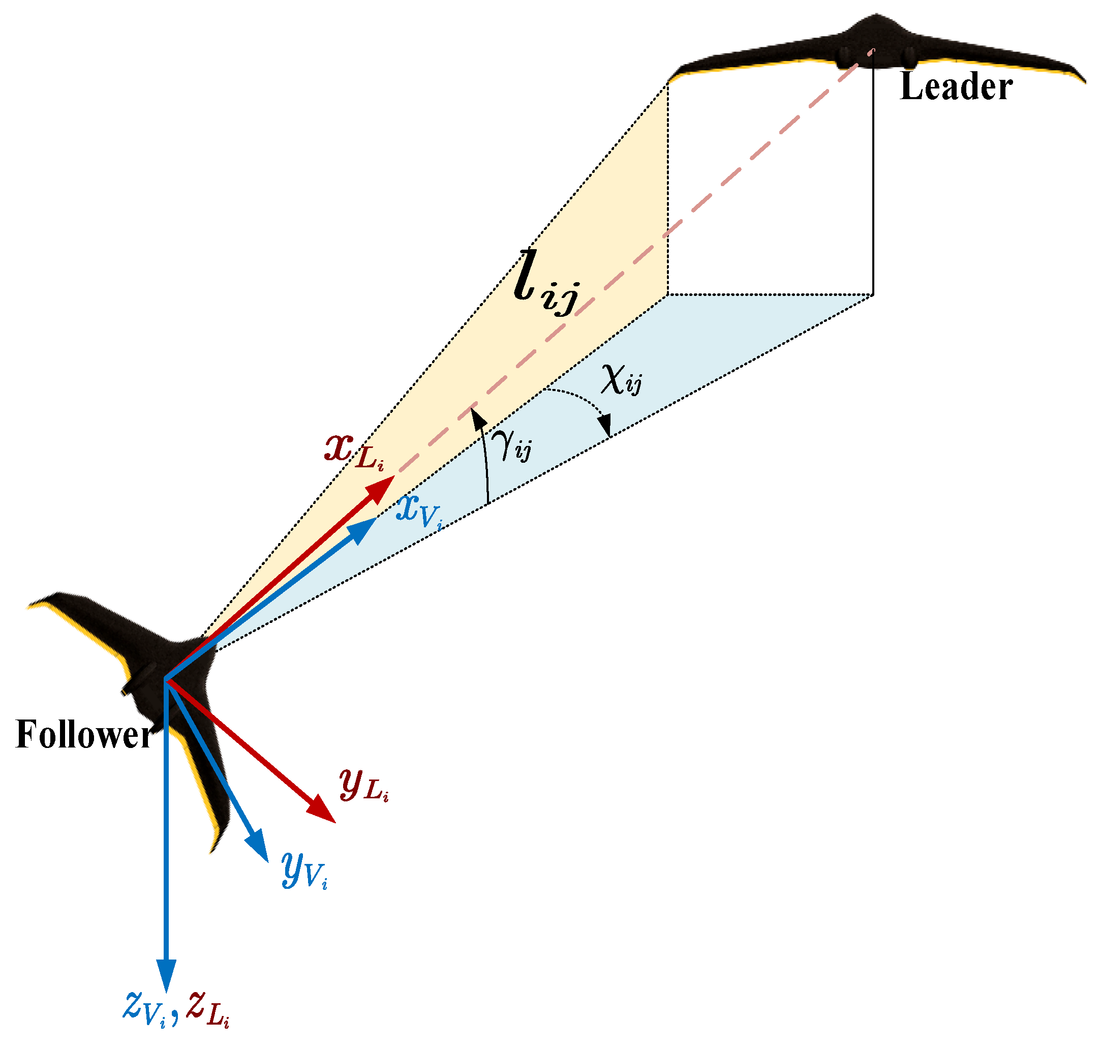
- The formation control problem of fixed-wing UAVs in an uncommunicated situation was studied. UAVs use only onboard vision sensors to obtain the status of UAVs in the neighborhood and to achieve formation control.
- (2)
- In this paper, we considered sensor measurements and used Extended Kalman Filtering to reduce errors and designed a sliding mode controller to reduce sensitivity to measurement errors.
- (3)
- In this paper, the formation control was divided into a two-layer control structure of position control and attitude control, and a suitable Lyapunov function was constructed to prove the system’s stability.
- (4)
- The UAV state transfer delay was considered, the UAV error state equation was given, and a suitable Lyapunov- Krasovskii generalized function was constructed to derive sufficient conditions for the stability of the delayed system, and finally, the obtained theoretical results were illustrated by three numerical simulations.
2. Extended Kalman Filter-Based State Estimation
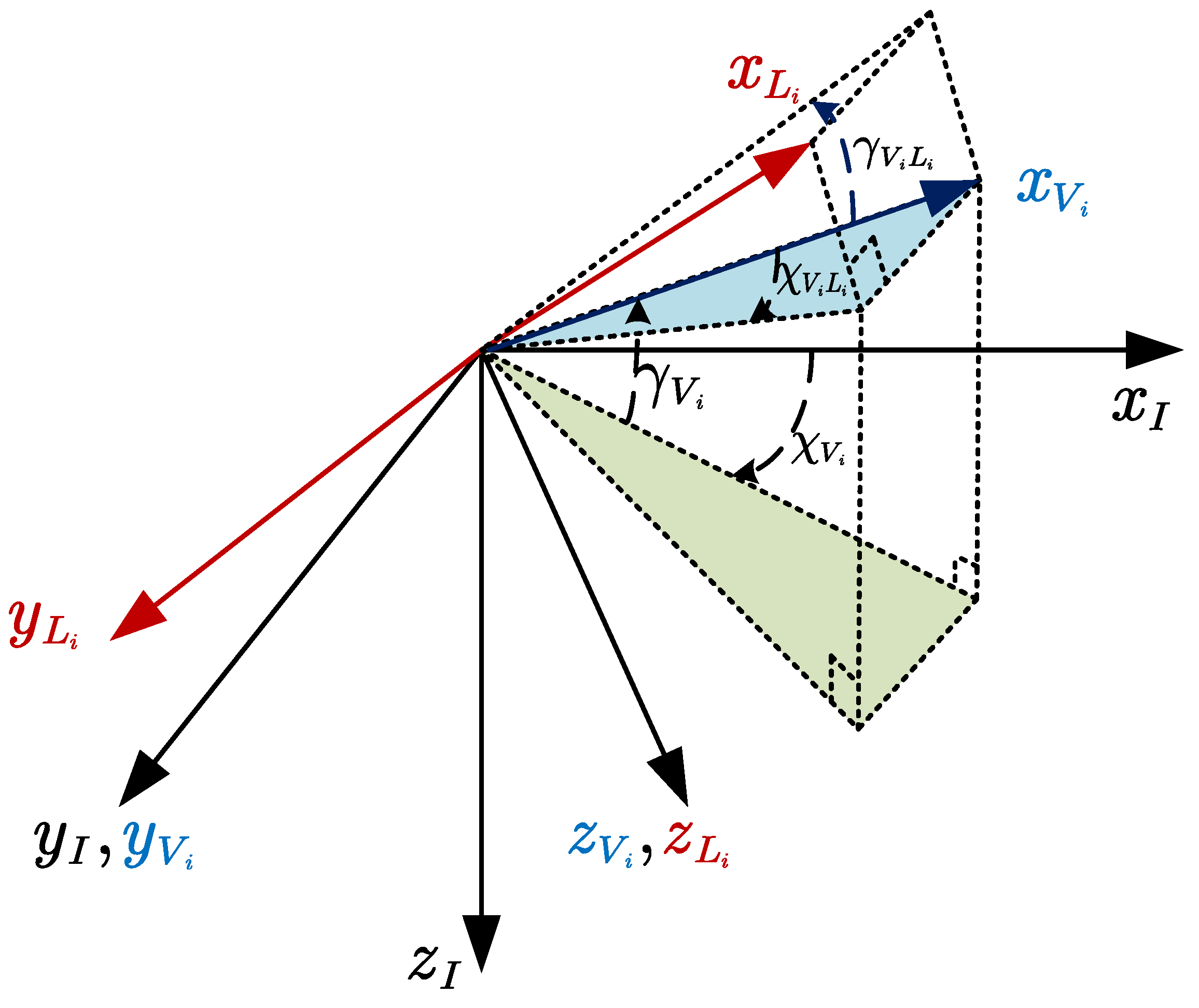
2.1. Equation of Motion for Single Machine
2.2. Leader UAV Status Estimation
3. Controller Design
3.1. Controller Design
3.2. System Stability Proof
3.3. Delayed System Stability Proof
4. Simulation and Test Results
4.1. Case 1
4.2. Case 2
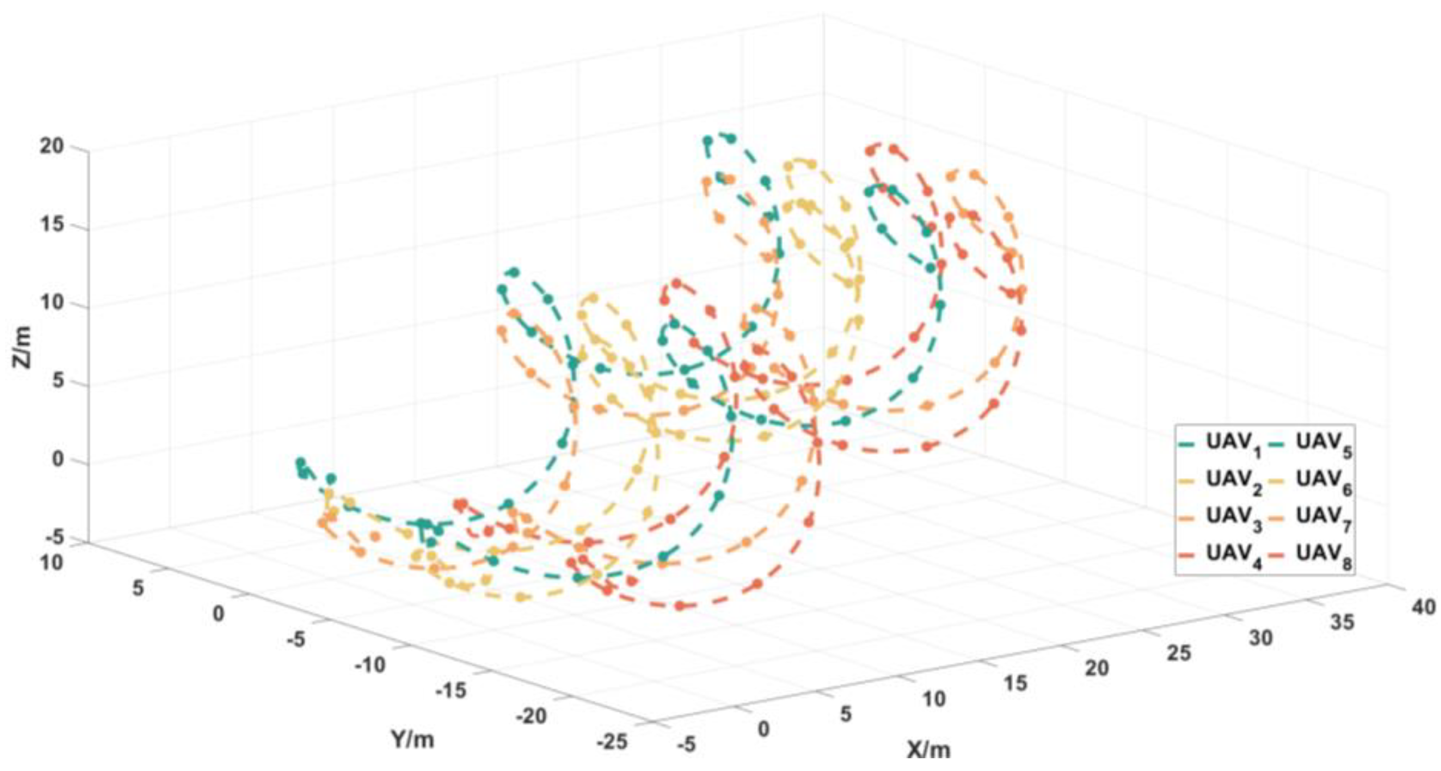
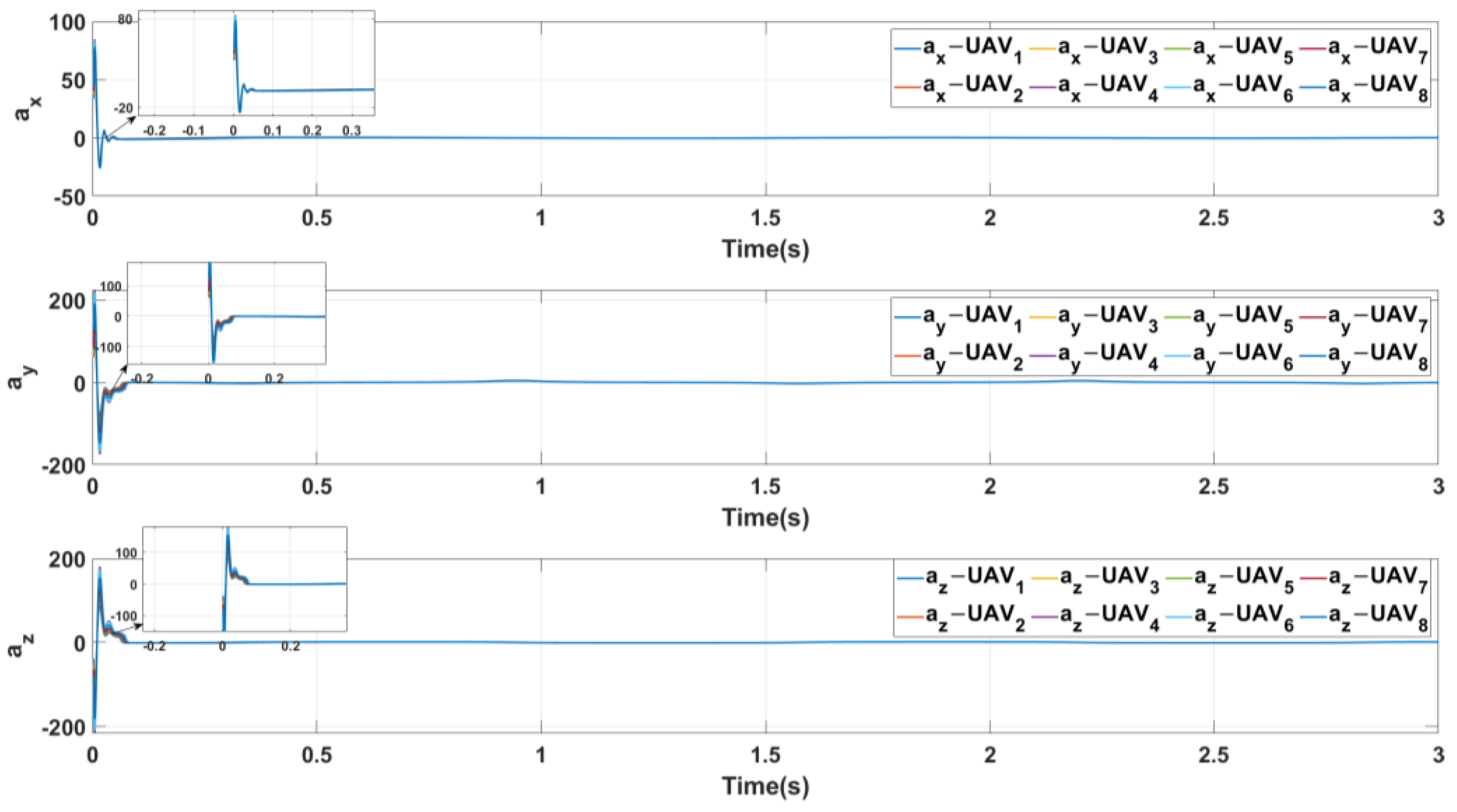
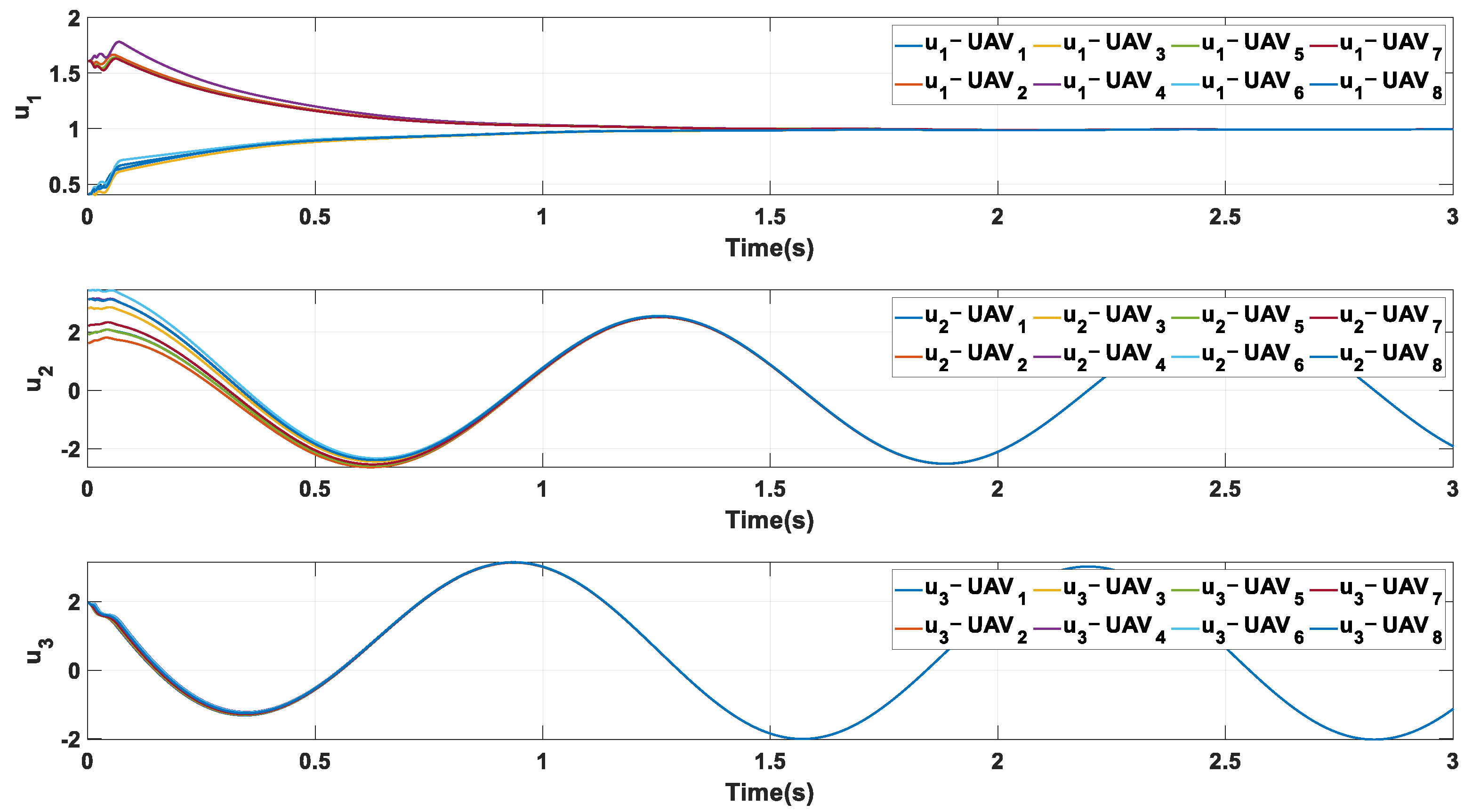
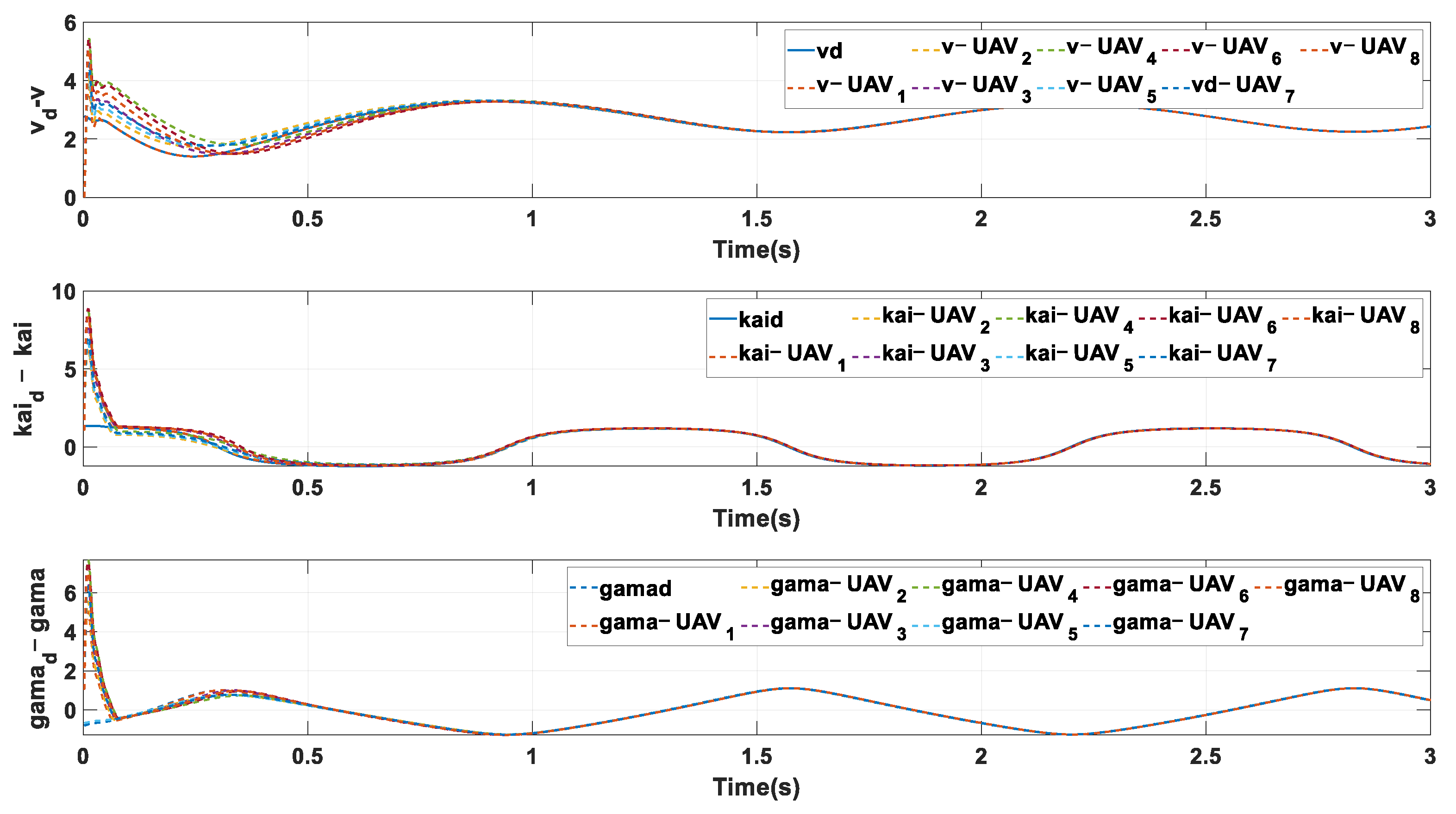
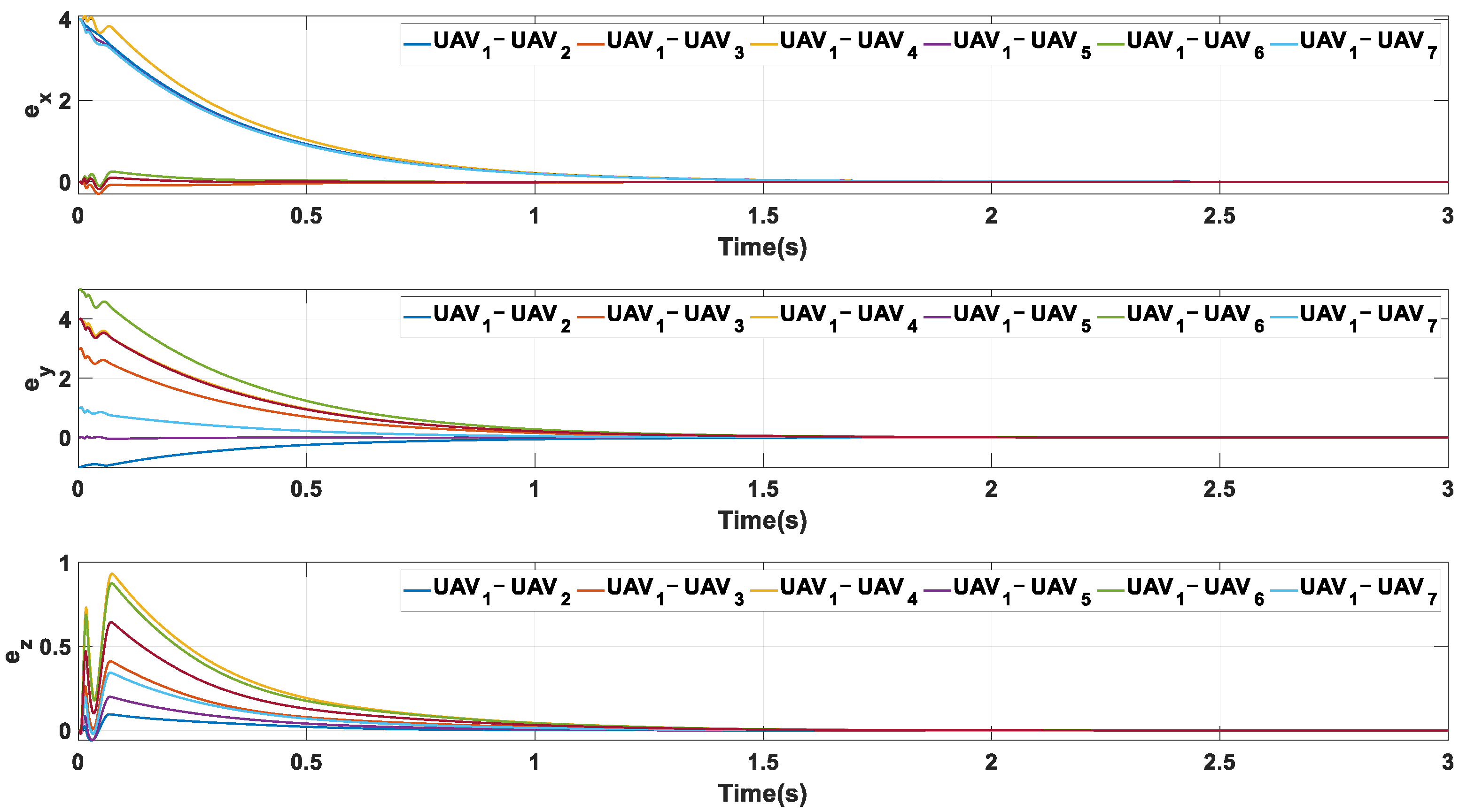
4.3. Case 3
4.4. Discussion
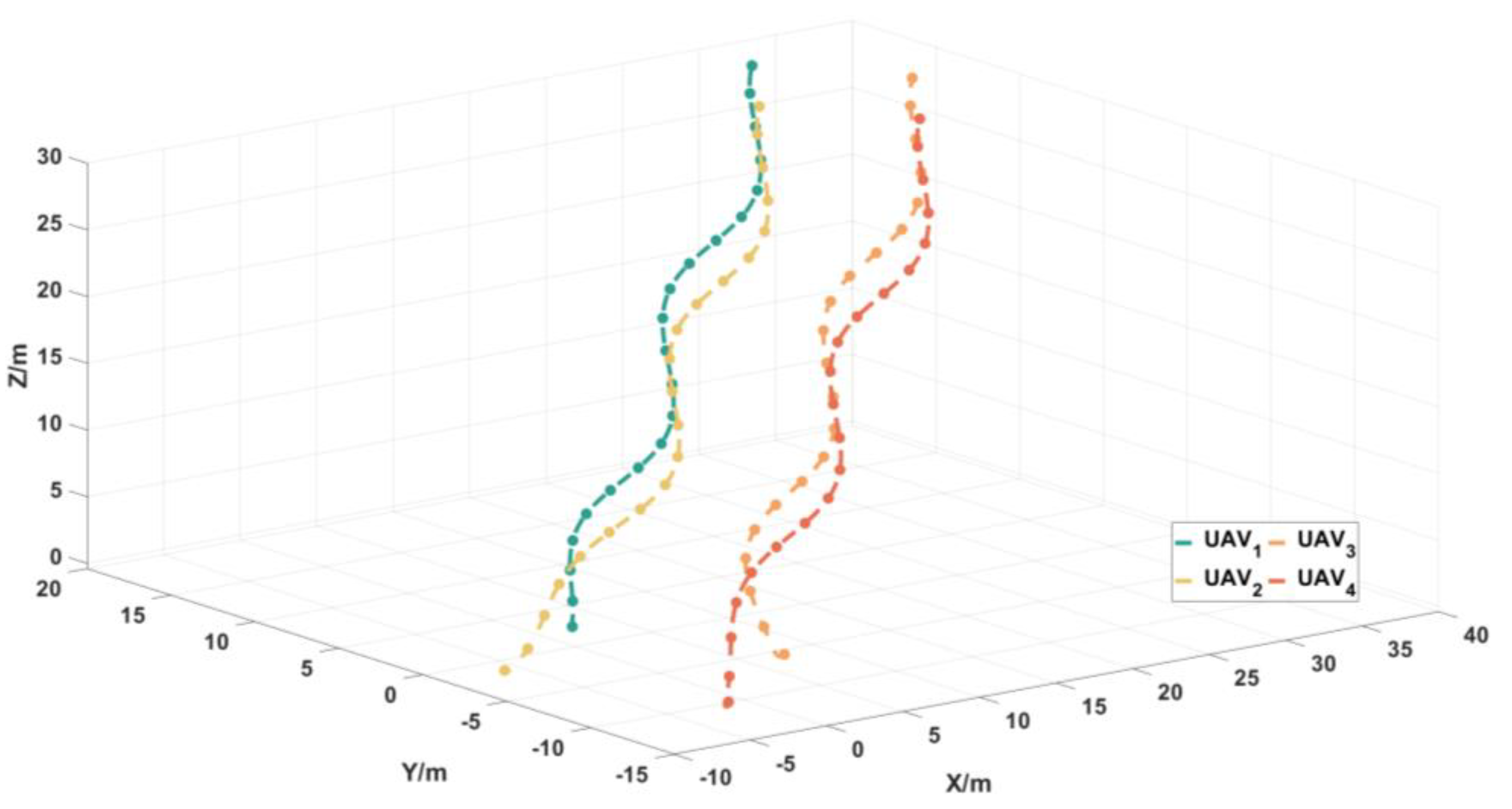
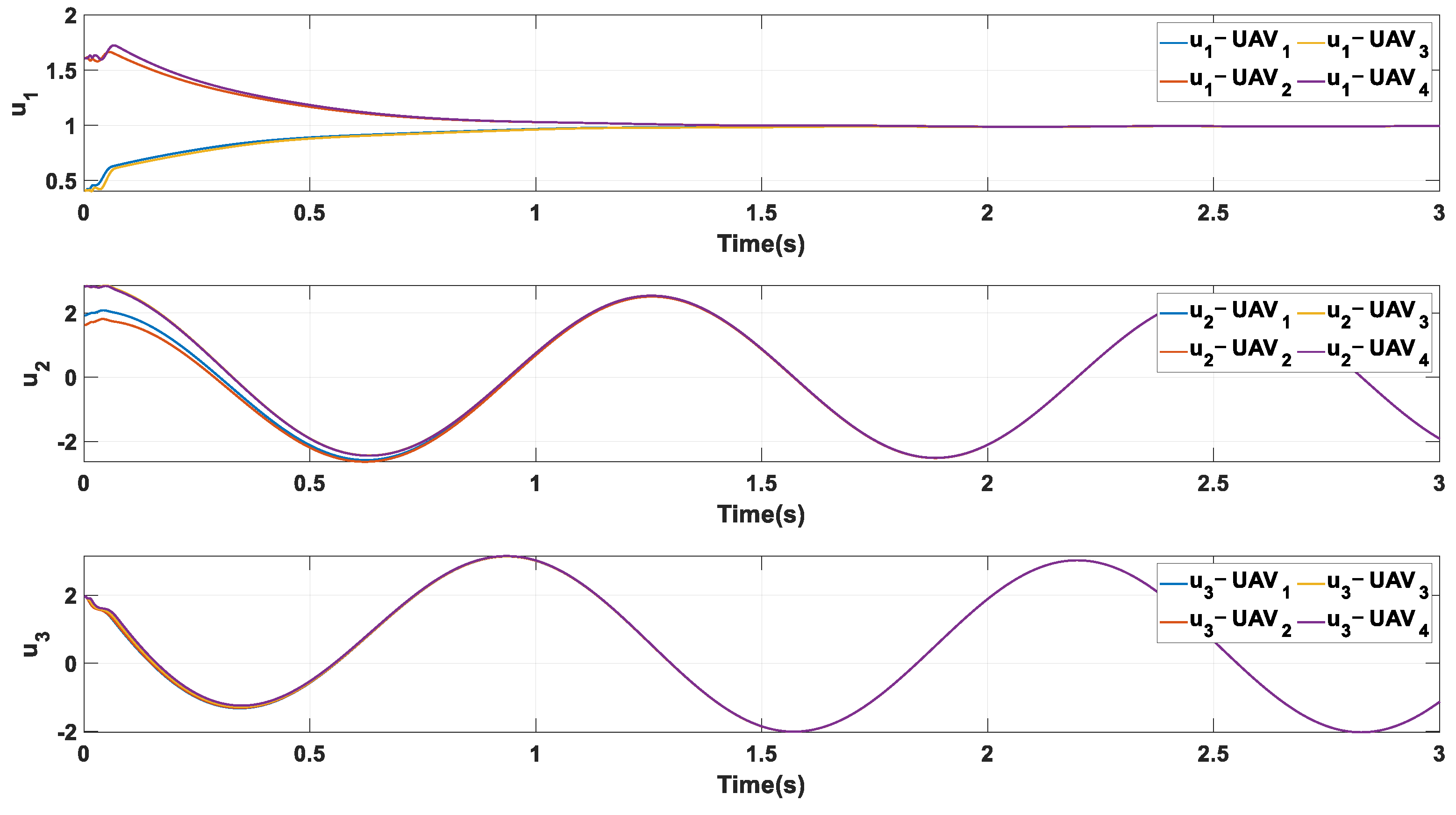
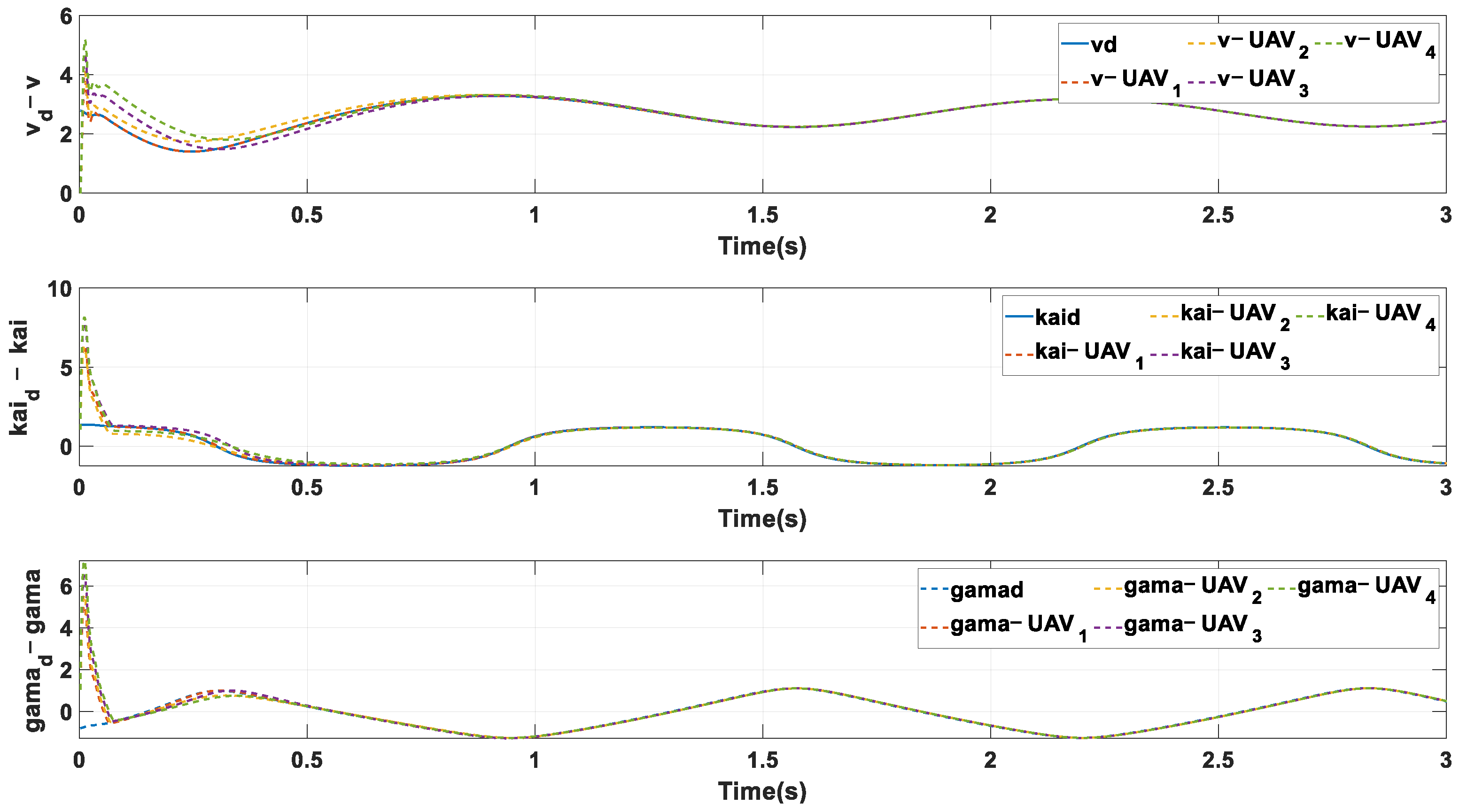
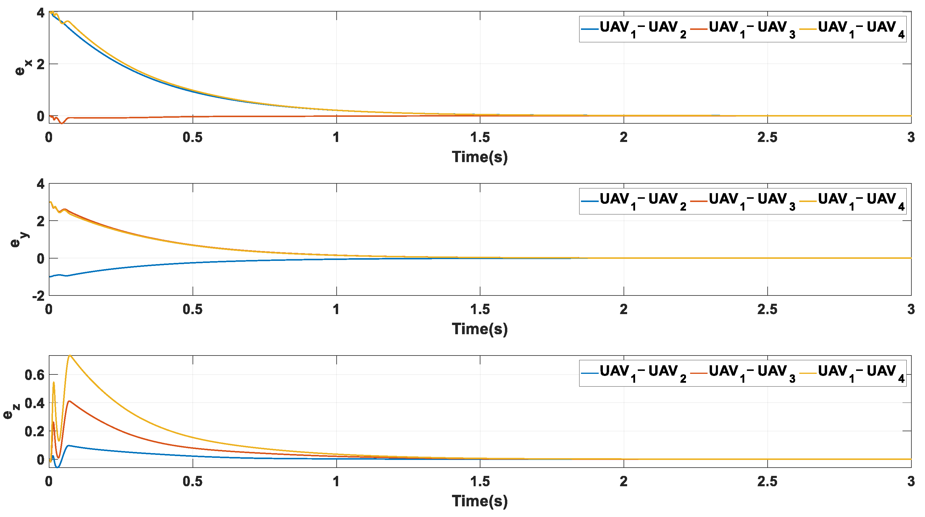
- The designed controller can be effectively applied to the formation control of fixed-wing UAVs, even in the presence of measurement errors as well as state transfer time delays in multiple UAV formations.
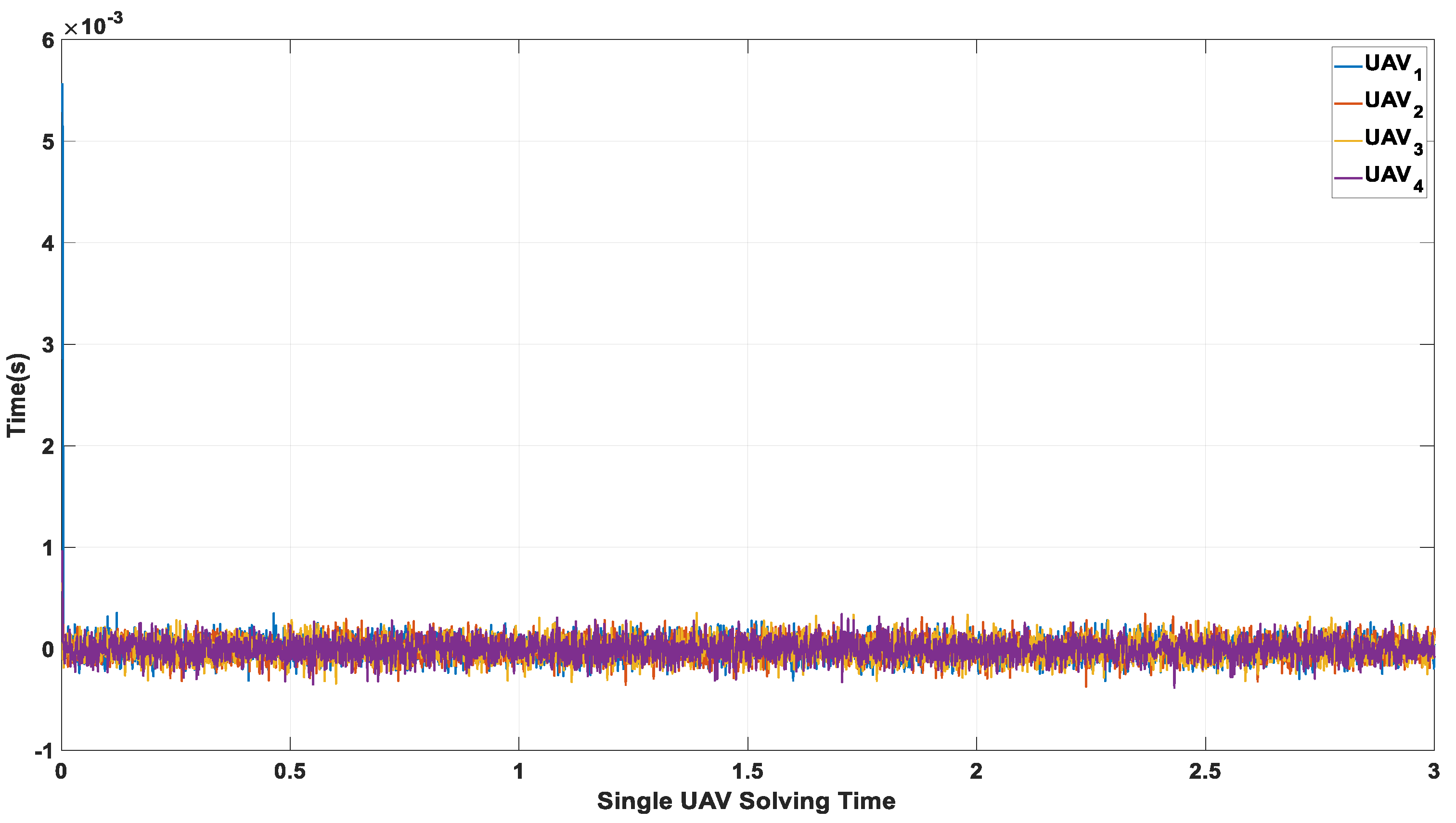
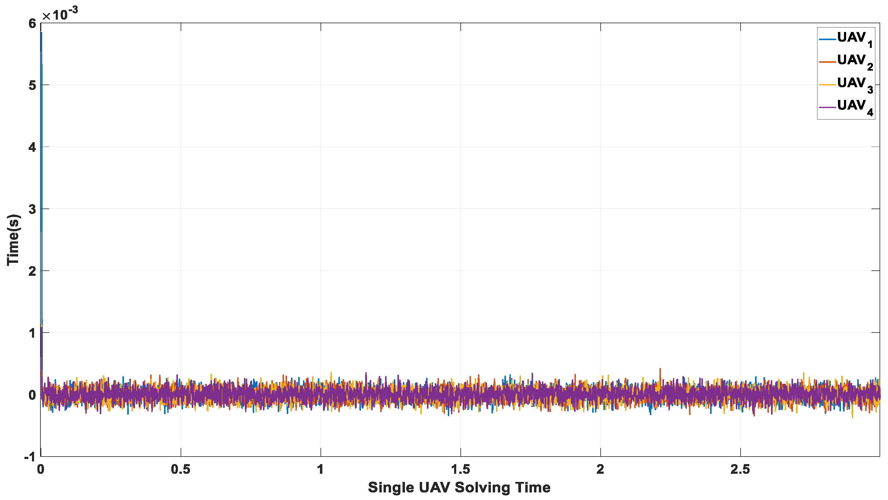
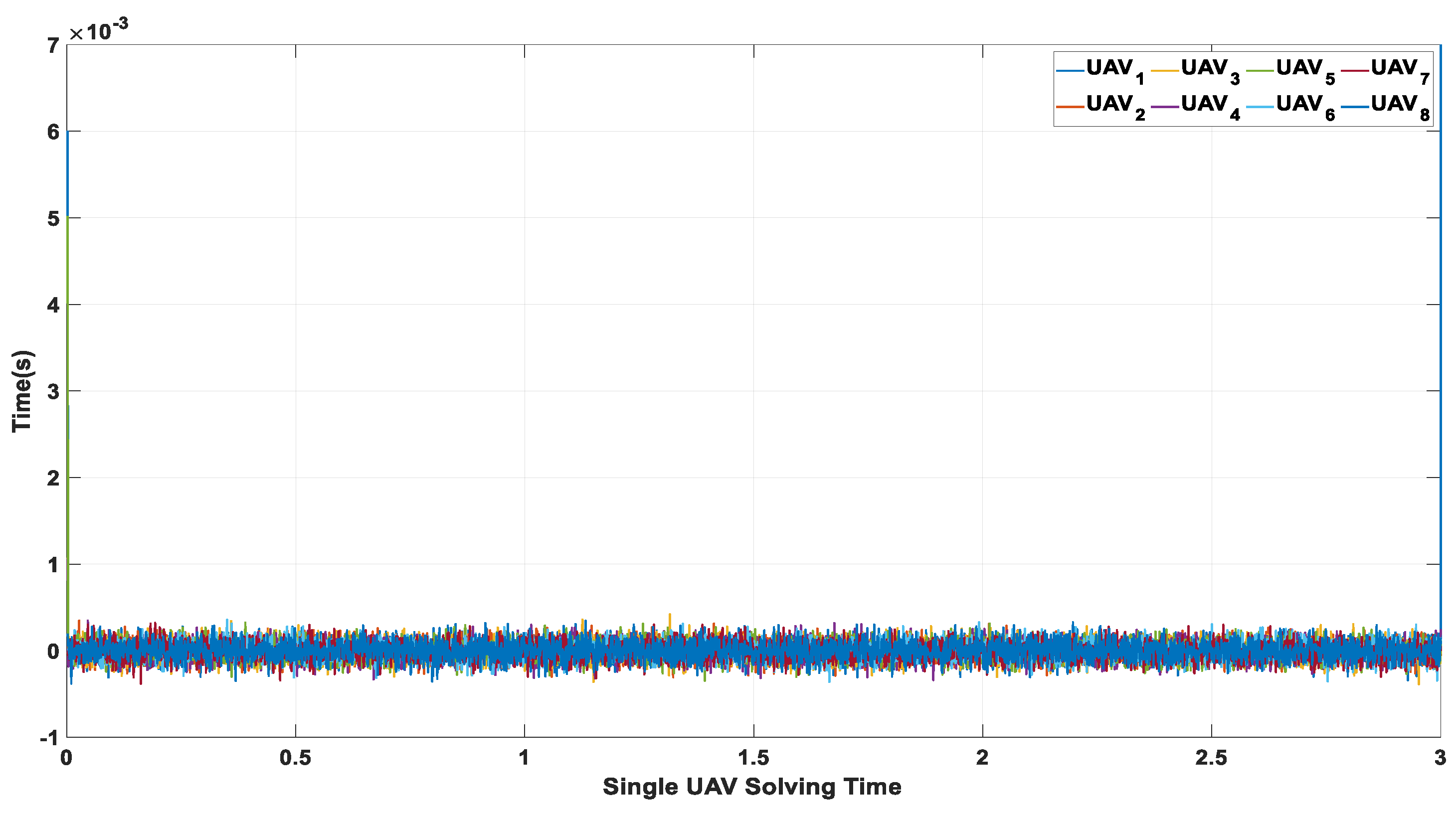
- It can be seen from the computation times of the three examples that, since the controller was distributed, it did not increase the solution time of individual UAVs as the number of UAVs increased. However, there was a long initial moment at the beginning of each phase in the time of each numerical simulation, which would be the next step to improve.
- When there were multiple UAVs in the neighborhood, the selection of the follower UAV for the desired leader UAV became an issue. In the next step of the study, rules need to be developed or the research method updated to ensure the efficiency and accuracy of the follower UAV’s selection of the desired leader UAV.
5. Conclusions
Author Contributions
Funding
Data Availability Statement
Conflicts of Interest
References
- Alsamhi, S.H.; Shvetsov, A.V.; Kumar, S.; Shvetsova, S.V.; Alhartomi, M.A.; Hawbani, A.; Rajput, N.S.; Srivastava, S.; Saif, A.; Nyangaresi, V.O. UAV Computing-Assisted Search and Rescue Mission Framework for Disaster and Harsh Environment Mitigation. Drones 2022, 6, 154. [Google Scholar] [CrossRef]
- Radmanesh, M.; Kumar, M. Flight formation of UAVs in presence of moving obstacles using fast-dynamic mixed integer linear programming. Aerosp. Sci. Technol. 2016, 50, 149–160. [Google Scholar] [CrossRef] [Green Version]
- Madyastha, V.K.; Caliset, A.J. An adaptive filtering approach to target tracking. In Proceedings of the American Control Conference, Portland, OR, USA, 8–10 June 2005. [Google Scholar]
- Alsamhi, S.H.; Shvetsov, A.V.; Kumar, S.; Hassan, J.; Alhartomi, M.A.; Shvetsova, S.V.; Sahal, R.; Hawbani, A. Computing in the Sky: A Survey on Intelligent Ubiquitous Computing for UAV-Assisted 6G Networks and Industry 4.0/5.0. Drones 2022, 7, 177. [Google Scholar] [CrossRef]
- Alsamhi, S.H.; Ma, O.; Ansari, M.S.; Gupta, S.K. Collaboration of Drone and Internet of Public Safety Things in Smart Cities: An Overview of QoS and Network Performance Optimization. Drones 2019, 3, 13. [Google Scholar] [CrossRef] [Green Version]
- Desai, J.P.; Ostrowski, J.P.; Kumar, V. Modeling and control of formations of nonholonomic mobile robots. IEEE Trans. Robot. Autom. 2001, 17, 905–908. [Google Scholar] [CrossRef] [Green Version]
- Roldão, V.; Cunha, R.; Cabecinhas, D.; Silvestre, C.; Oliveira, P. A leader-following trajectory generator with application to quadrotor formation flight. Robot. Auton. Syst. 2014, 62, 1597–1609. [Google Scholar] [CrossRef]
- Fierro, R.; Belta, C.; Desai, J.P.; Kumar, V. On controlling aircraft formations. In Proceedings of the 40th IEEE Conference on Decision and Control (Cat. No.01CH37228), Orlando, Fl, USA, 4–7 December 2001; Volume 2, pp. 1065–1070. [Google Scholar]
- Eren, T. Formation shape control based on bearing rigidity. Int. J. Control. 2012, 85, 1361–1379. [Google Scholar] [CrossRef]
- Lewis, M.A.; Tan, K.H. High precision formation control of mobile robots using virtual structures. Auton. Robots. Auton. Robot. 1997, 4, 387–403. [Google Scholar] [CrossRef]
- Sharma, R.; Ghose, D. Collision avoidance between UA V clusters using swarm intelligence techniques. Int. J. Syst. Sci. 2009, 5, 521–538. [Google Scholar] [CrossRef]
- Giulietti, F.; Innocenti, M.; Pollini, L. Formation flight control—A behavioral approach. In Proceedings of the AIAA Guidance, Navigation, and Control Conference and Exhibit, Montreal, QC, Canada, 6–9 August 2001. [Google Scholar]
- Park, C.; Tahk, M.; Bang, H. Multiple Aerial Vehicle Formation Using Swarm Intelligence. In Proceedings of the AIAA Guidance, Navigation, and Control Conference and Exhibit, Austin, TX, USA, 11–14 August 2003. [Google Scholar]
- Ren, W. Consensus based formation control strategies for multi-vehicle systems. In Proceedings of the 2006 American Control Conference, Minneapolis, MN, USA, 14–16 June 2006. [Google Scholar]
- Jadbabaie, A.; Lin, J.; Morse, A.S. Coordination of groups of mobile autonomous agents using nearest neighbor rules. IEEE Trans. Autom. 2003, 6, 988–1001. [Google Scholar] [CrossRef] [Green Version]
- Wang, X.; Yu, Y.; Li, Z. Distributed sliding mode control for leader-follower formation flight of fixed-wing unmanned aerial vehicles subject to velocity constraints. Int. J. Robust Nonlinear Control 2021, 31, 2110–2125. [Google Scholar] [CrossRef]
- Liu, S.; Tan, D.; Liu, G. Robust Leader-follower Formation Control of Mobile Robots Based on a Second Order Kinematics Model. Acta Autom. Sin. 2007, 33, 947–955. [Google Scholar] [CrossRef] [Green Version]
- Zhao, C.; Dai, S.; Zhao, G.; Gao, C.; Liu, S. UAV formation control based on distributed model predictive control. Control. Decis. 2021, 1, 1–9. [Google Scholar]
- Kim, S.; Cho, H.; Jung, D. Evaluation of Cooperative Guidance for Formation Flight of Fixed-wing UAVs using Mesh Network. In Proceedings of the 2020 International Conference on Unmanned Aircraft Systems, Athens, Greece, 1–4 September 2020. [Google Scholar]
- Parivallal, A.; Sakthivel, R.; Amsaveni, R.; Alzahrani, F.; Alshomrani, A.S. Observer-based memory consensus for nonlinear multi-agent systems with output quantization and Markov switching topologies. Phys. A Stat. Mech. Its Appl. 2020, 551, 123949. [Google Scholar] [CrossRef]
- Sakthivel, R.; Parivallal, A.; Huy Tuan, N.; Manickavalli, S. Nonfragile control design for consensus of semi-Markov jumping multiagent systems with disturbances. Int. J. Adapt. Control. Signal Process. 2021, 35, 1039–1061. [Google Scholar] [CrossRef]
- Polloni, L.; Mati, R.; Innocenti, M.; Campa, G.; Napolitano, M. A Synthetic Environment for the Simulation of Visionbased Formation Flight. In Proceedings of the AIAA Modeling and Simulation Technologies Conference, Austin, TX, USA, 11–14 August 2003. [Google Scholar]
- Ray, R.; Cobleigh, B.; Vachon, M.; St John, C. Flight Test Techniques used to Evaluate Performance Benefits During Formation Flight. In Proceedings of the AIAA Atmospheric Flight Mechanics Conference and Exhibit, Monterey, CA, USA, 5–8 August 2002. [Google Scholar]
- Seanor, B.; Campa, G.; Gu, Y.; Napolitano, M.; Rowe, L.; Perhinschi, M. Formation Flight Test Results for UAV Research Aircraft Models. In Proceedings of the AIAA 1st Intelligent Systems Technical Conference, Chicago, IL, USA, 20–22 September 2004. [Google Scholar]
- Sattigeri, R.; Calise, A.; Kim, B.S.; Volyanskyy, K.; Kim, N. 6-DOF Nonlinear Simulation of Vision-Based Formation Flight. In Proceedings of the AIAA Guidance, Navigation, and Control Conference and Exhibit, San Francisco, CA, USA, 15–18 August 2005. [Google Scholar]
- Lin, J.; Miao, Z.; Zhong, H.; Peng, W.; Wang, Y.; Fierro, R. Adaptive Image-Based Leader-Follower Formation Control of Mobile Robots with Visibility Constraints. IEEE Trans. Ind. Electron. 2021, 68, 6010–6019. [Google Scholar] [CrossRef]
- Chen, X.; Jia, Y. Adaptive leader-follower formation control of nonholonomic mobile robots using active vision. IET Control. Theory Appl. 2015, 8, 1302–1311. [Google Scholar] [CrossRef]
- Sattigeri, R.; Calise, A.J.; Evers, J.H. An adaptive vision-based approach to decentralized formation control. J. Aerosp. Comput. Inf. Commun. 2004, 1, 502–525. [Google Scholar] [CrossRef] [Green Version]
- Chen, Q.; Jin, Y.; Wang, T.; Wang, Y.; Yan, T.; Long, Y. UAV Formation Control Under Communication Constraints Based on Distributed Model Predictive Control. IEEE Access 2022, 2022, 126494–126507. [Google Scholar]
- Qin, J.; Zhang, G.; Zheng, W.X.; Kang, Y. Adaptive Sliding Mode Consensus Tracking for Second-Order Nonlinear Multiagent Systems with Actuator Faults. IEEE Trans. Cybern. 2019, 49, 1605–1615. [Google Scholar] [CrossRef]
- Desai, J.P.; Ostrowski, J.; Kumar, V. Controlling formations of multiple mobile robots. In Proceedings of the IEEE Transactions on Robotics & Automation, Leuven, Belgium, 20 May 2010; Volume 6, pp. 905–908. [Google Scholar]
- Das, A.K.; Fierro, R.; Kumar, V.; Ostrowski, J.P.; Spletzer, J.; Taylor, C.J. A vision-based formation control framework. IEEE Trans. Robot. Autom. 2002, 18, 813–825. [Google Scholar] [CrossRef] [Green Version]
- Mariottini, G.L.; Morbidi, F.; Prattichizzo, D.; Vander Valk, N.; Michael, N.; Pappas, G.; Daniilidis, K. Vision-Based Localization for Leader-Follower Formation Control. IEEE Trans. Robot. 2009, 25, 1431–1438. [Google Scholar] [CrossRef]
- Galzi, D.; Shtessel, Y. UAV formations control using high order sliding modes. In Proceedings of the American Control Conference, Minneapolis, MN, USA, 14–16 June 2006. [Google Scholar]
- Kadungoth Sreeraj, A.R. A Model-Free Control Algorithm Based on the Sliding Mode Control Method with Applications to Unmanned Aircraft Systems. Ph.D. Thesis, Rochester Institute of Technology, Rochester, NY, USA, 2019. [Google Scholar]
- Mobayen, S. Adaptive Global Terminal Sliding Mode Control Scheme with Improved Dynamic Surface for Uncertain Nonlinear Systems. Int. J. Control. Autom. Syst. 2018, 16, 1692–1700. [Google Scholar] [CrossRef]
- Dehghani, M.A.; Menhaj, M.B. Integral sliding mode formation control of fixed-wing unmanned aircraft using seeker as a relative measurement system. Aerosp. Sci. Technol. 2016, 58, 318–327. [Google Scholar] [CrossRef]
- Ailon, A.; Zohar, I. Controllers for trajectory tracking and string-like formation in Wheeled Mobile Robots with bounded inputs. In Proceedings of the Melecon 2010–2010 15th IEEE Mediterranean Electrotechnical Conference, Valletta, Malta, 26–28 April 2010. [Google Scholar]


| Parameter Name | Symbols | Numerical Value |
|---|---|---|
| Sampling interval | 0.01 | |
| Sampling time | 30 | |
| Number of drones | 4 | |
| Intermachine delay | 0.004 |
| UAV Number | Initial Location | Yaw Angle | |
|---|---|---|---|
| 1 | 0 | ||
| 2 | 0 | ||
| 3 | 0 | ||
| 4 | 0 |
| UAV Number | Initial Location | Yaw Angle | |
|---|---|---|---|
| 1 | 0 | ||
| 2 | 0 | ||
| 3 | 0 | ||
| 4 | 0 | ||
| 5 | 0 | ||
| 6 | 0 | ||
| 7 | 0 | ||
| 8 | 0 |
Disclaimer/Publisher’s Note: The statements, opinions and data contained in all publications are solely those of the individual author(s) and contributor(s) and not of MDPI and/or the editor(s). MDPI and/or the editor(s) disclaim responsibility for any injury to people or property resulting from any ideas, methods, instructions or products referred to in the content. |
© 2023 by the authors. Licensee MDPI, Basel, Switzerland. This article is an open access article distributed under the terms and conditions of the Creative Commons Attribution (CC BY) license (https://creativecommons.org/licenses/by/4.0/).
Share and Cite
Chen, Q.; Wang, T.; Jin, Y.; Wang, Y.; Qian, B. A UAV Formation Control Method Based on Sliding-Mode Control under Communication Constraints. Drones 2023, 7, 231. https://doi.org/10.3390/drones7040231
Chen Q, Wang T, Jin Y, Wang Y, Qian B. A UAV Formation Control Method Based on Sliding-Mode Control under Communication Constraints. Drones. 2023; 7(4):231. https://doi.org/10.3390/drones7040231
Chicago/Turabian StyleChen, Qijie, Taoyu Wang, Yuqiang Jin, Yao Wang, and Bei Qian. 2023. "A UAV Formation Control Method Based on Sliding-Mode Control under Communication Constraints" Drones 7, no. 4: 231. https://doi.org/10.3390/drones7040231