High Precision Mesh-Based Drone Image Stitching Based on Salient Structure Preservation and Regular Boundaries

Abstract

Addressing problems such as obvious ghost, dislocation, and distortion resulting from the traditional stitching method, a novel drone image-stitching method is proposed using mesh-based local double-feature bundle adjustment and salient structure preservation which aims to obtain more natural panoramas.The proposed method is divided into the following steps. First, reducing parallax error is considered from both global and local aspects. Global bundle adjustment is introduced to minimize global transfer error, and then the local mesh-based feature-alignment model is incorporated into the optimization framework to achieve more accurate alignment. Considering the sensitivity of human eyes to linear structure, the global linear structure that runs through the images obtained by segment fusion is introduced to prevent distortions and align matching line segments better. Rectangular panoramas usually have better visual effects. Therefore, regular boundary constraint combined with mesh-based shape-preserving transform can make the results more natural while preserving mesh geometry. Two new evaluation metrics are also developed to quantify the performance of linear structure preservation and the alignment difference of matching line segments. Extensive experiments show that our proposed method can eliminate parallax and preserve global linear structures better than other state-of-the-art stitching methods and obtain more natural-looking stitching results.

1. Introduction

In recent years, unmanned aerial vehicles (UAVs) have become more and more popular because of their fast, flexible, compact, and low-cost characteristics. They has been widely used in environmental monitoring [1], aerial imaging [2], disaster assessment [3], and other fields. Limited by the flying height of the UAVs and the focal length of the digital camera, the imaging area of a single image is limited, so it is necessary to stitch a series of overlapping UAV images into a panorama with a wider field of vision.

In order to obtain natural panorama, most of the current methods are to build an accurate alignment model to reduce parallax error, and according to the method of obtaining the alignment model, UAV image stitching can be divided into image-based stitching and pose information-based image stitching. UAV image stitching based on pose information usually requires extra information, such as camera parameters, global navigation satellite systems (GNSSs), inertial measurement units (IMUs), and ground control points (GCPs); the accuracy of these information directly affects the quality of the stitching results [1,2,3,4,5]; image-based stitching does not need this information [6,7,8,9]. Our proposed method can obtain visually satisfactory stitching results automatically, without the requirements of extra information such as camera calibration parameters and camera poses.

The process of image-based stitching can be roughly summarized as image matching, extracting reliable corresponding points, constructing an alignment model according to the corresponding points, and then blending the warped images, e.g., through multi-band blending, linear blending, etc.

Image matching is the process of identifying the same or similar content and structure from two or more images and corresponding them. It can be roughly divided into two categories, area-based and feature-based matching [10]. Generally, feature-based methods are used in image stitching, and its basic process can be summarized as feature point extraction, (such as scale invariant features transform (SIFT) [11], sped-up robust features (SURF) [12], oriented FAST, rotated BRIEF (ORB) [13], descriptor construction, and feature-point matching. At this time, there are still a large number of mismatching points in the feature point set, that is, outer points. Therefore, in order to improve the matching accuracy, it is necessary to remove the mismatching. The most commonly used is the random sample consensus (RANSAC) proposed by Fischler and Bolles [14] and its improved algorithms [15,16]. This can find inner points from a set of data sets containing “outer points” and estimate global model parameters. In recent years, some non-rigid image-matching models have been proposed, such as locality-preserving matching (LPM) [17] and its variety, local graph structure consensus (LGSC) [18]. They can remove mismatches based on the assumption of locality. In addition, a learning-based technique has also been widely studied to remove outliers. For example, Yi et al. [19] proposed learning to find good correspondences (LFGC) which could find good feature correspondences by training a network from a set of putative match sets together with their image intrinsics; Ma et al. [20] proposed a two-class classifier based on learning (LMR) to remove mismatches by using a few training image pairs and handcrafted geometrical representations for training and testing. Image matching can provide more accurate points correspondence for the next stitching step, which is an important step of image stitching.

The purpose of image stitching is to stitch multiple images with overlapping areas into a panorama [21]. Early image stitching used a global transformation (usually a global homography matrix) to minimize alignment errors, such as AutoStitch [22] proposed by Brown and Lowe; this method is robust, but not flexible enough. It is only suitable for planar or parallax free scenes. Violating the above assumptions will lead to dislocation, ghost and other problems.

To improve the accuracy of alignment, Lin et al. [23] proposed a smoothly varying affine (SVA) warp, which replaces the global affine warp by a smoothly affine stitching field; Zaragoza et al. [24] proposed an as-projective-as-possible (APAP) warp, which estimates the local alignment model based on the global alignment to improve the alignment accuracy. Combing with seam cutting can obtain the optimal local alignment. Zhang and Liu [25] proposed a parallax-tolerant warp, which finds the optimal homography through the seam and further use content-preserving warping to locally refine the alignment; Lin et al. [26] proposed a seam-guided local alignment (SEAGULL) warp which uses the estimated seam to guide the optimization of local alignment process and iteratively improves the seam quality, but these methods suffer from projection distortion.

To alleviate perspective distortion in non-overlapping areas, Chang et al. [27] proposed a shape-preserving half-projective (SPHP) warp, which combines homography warp and similarity warp to maintain good alignment in overlapping areas, and keep the original perspectives in the non-overlapping region; Lin et al. [28] proposed an as-natural-as-possible (AANAP) warp to solve the problem of unnatural rotation of SPHP which realizes a smoother transition from overlapping areas to non overlapping areas by linearly combining perspective transformation and similarity transformation which has the minimum rotation angle; Chen and Chuang [29] proposed a mesh-guided warp with the global similarity prior (GSP) which selects better rotation and scale for each image to minimize distortion. Li et al. [30] propose a novel quasi-homography warp, which effectively balances the perspective distortion against the projective distortion in the non-overlapping region to create a more natural-looking panorama; Li et al. [31] proposed a parallax-tolerant image-stitching method based on robust elastic warping which constructed an analytical warping function to eliminate the parallax errors and used global similarity transformation to mitigate distortion. They also applied a Bayesian model to remove incorrect local matching in order to ensure more robust alignment.

Human eyes are more sensitive to lines. Emphasizing double features can not only avoid the bending of line segments, but also improve the natural quality of the warped images [32,33]. Zhang et al. [34] proposed a mesh-based framework to stitch wide-baseline images, and designed a line-preserving term to prevent line segments from bending. Xiang et al. [35] presents a line-guided local warping method with a global similarity constraint which uses line features to strengthen geometric constraints and adopts a global similarity constraint to mitigate projective distortions. Liao and Li [36] proposed a mesh optimization algorithm based on double features (point features and line features) and a quasi homography model to solve the problems of alignment and distortion and emphasize the naturalness of stitching results; Jia et al. [37] proposed a dual-feature warp which obtains consistent point and line pairs by exploring co-planar subregions using projective invariants and incorporate global collinear structures as a constraint to preserve both local and global linear structures while alleviating distortions.

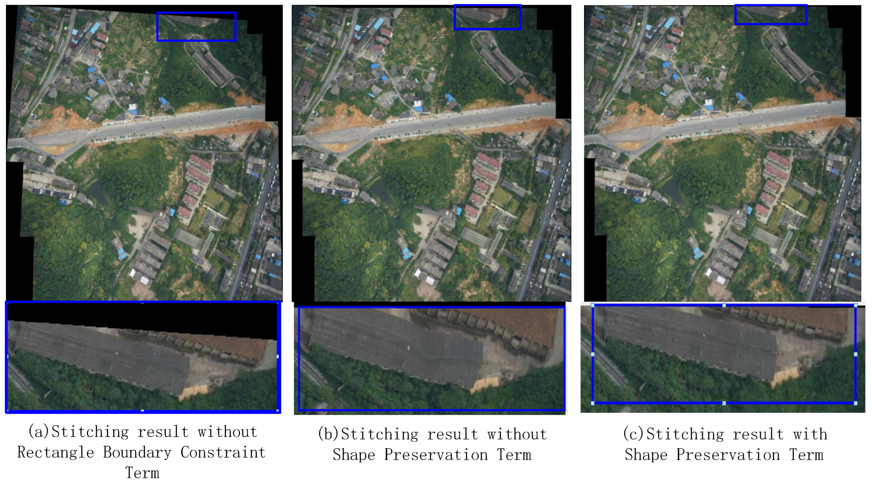
Most of the stitched panoramic images have irregular boundaries. For better visual effects, warping-based rectangular boundary optimization is proposed by He et al. [38], but it cannot deal with a scene that is not completely captured; Zhang et al. [39] proposed a mesh-based warp with regular boundary constraints, which incorporates line preservation and regular boundary constraints into the image-stitching framework, and conducts iterative optimizations to obtain an optimal piecewise rectangular boundary; Nie et al. [40] proposed the first deep learning solution to image rectangling which encourages the boundary rectangular mesh shape-preserving and perceptually natural content during iteration.

The traditional image-stitching method (such as AutoStitch) adopts global homography to align images and the stitching results usually have obvious ghosts, dislocations, and perspective distortions due to the insufficient flexibility of the homography. Then the mesh-based alignment model (such as APAP, SPHP, and AANAP) is introduced into the stitching framework to improve alignment accuracy and alleviate perspective distortions by assigning different homography to each mesh, but it may lead to structural distortions, such as line segments bending and irregular boundaries. Therefore, we propose a novel stitching strategy that can further reduce ghosts and dislocations while preventing structural distortions and obtain more natural stitching results with a regular boundary.

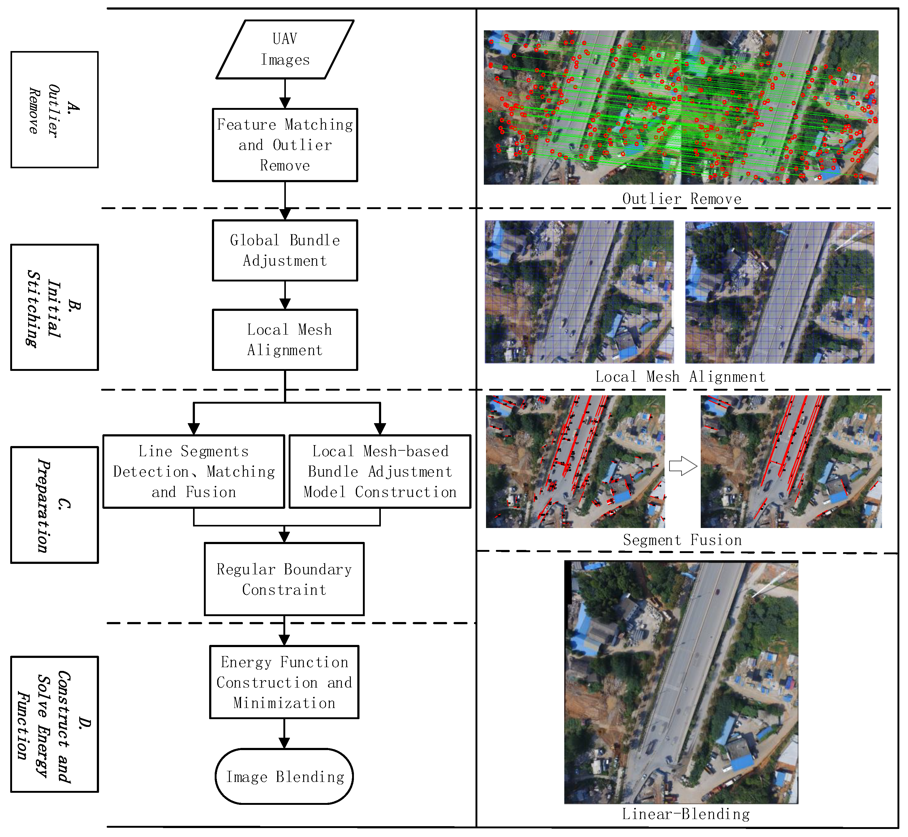
In this paper, an effective and robust mesh-based image stitching method is proposed to obtain more natural and accurate stitching results. The main idea of our proposed method can be summarized as improving alignment accuracy, preserving salient structure, and making the stitching results more natural. For alignment, parallax error is reduced from global and local aspects. First, global bundle adjustment is adopted to obtain a more accurate homography matrix and then the mesh-based local bundle adjustment feature alignment model is constructed to reduce parallax error further which is realized by minimizing energy function. For the preservation of salient structure, we try to merge local line segments into global line segments that run through the images and design energy functions guided by global collinear structure to preserve linear structure and align matching line segments. Finally, we emphasize the naturalness of the stitching results through boundary constraint and shape-preserving transform. The experimental results are fully compared and analyzed, including two new quantitative linear structure evaluation metrics.

The main contributions of this paper are summarized as:

• A novel image-stitching method is designed using a comprehensive strategy involving global bundle adjustment and a local mesh-based alignment model which can reduce the global transfer error through global bundle adjustment, and reduce the local parallax error by constructing mesh-based local feature alignment energy functions.
• New energy functions guided by a global collinear structure are designed to prevent global linear structure distortions and improve the performance of line segments alignment, addressing the decline of stitching quality caused by salient structural distortions. Furthermore, regular boundary constraint combined with mesh-based shape-preserving transform is introduced to obtain more natural stitching results.
• Two new quantitative evaluation metrics of linear structure are developed to quantify the preservation and alignment performance of linear structure for image stitching. Comprehensive experimental results and comparisons show that our proposed method is superior to some existing image-stitching methods.

The rest of this paper is introduced as follows. Section 2 introduces the method we propose in this paper; Section 3 evaluates the stitching results in terms of alignment accuracy, time efficiency and structure preservation qualitatively and quantitatively; Section 4 summarizes the work done and analyzes the current challenges of drone image stitching.

2. Methodology

In this section, we will introduce our image-stitching method in detail. First, we use SIFT [11] to extract feature points and obtain initial feature sets by matching (including a large number of outer points), and then adopt LGSC [18] to remove false matching. The global homography matrix cannot accurately align images. Thus, local mesh alignment is designed to obtain more accurate pre-warping images. Then original line segments is detected by LSD [41]. Longer line segments are obtained by merging short line segments. The boundary of the initial stitching results is extracted to prepare for the next energy terms construction. In the case of multi-image stitching, bundle adjustment is adopted to reduce parallax error from both global and local aspects. Different energy terms are constructed and the total energy function is minimized to obtain the final warping images, and finally linear blending is adopted to blend the warping images. The flowchart of our proposed stitching method is shown in Figure 1. Based on our proposed method, we can obtain a natural-looking and pleasant panorama.

2.1. Initial Image Stitching

Let I and $I^{\prime }$ denote the target image and the reference image, respectively. The correspondence of feature points $p=\left(x,y\right)\in I,p^{\prime }=\left(x^{\prime },y^{\prime }\right)\in I^{\prime }$ between target image and reference image can be represented by global homography, which can be expressed as:

$$\begin{array}{c}\hfill p^{\prime }\sim H·p\end{array}$$

(1)

where $H\in R^{3\times 3}$

$$H=\left[\begin{array}{ccc}{h}_1& h_2& h_3\\ h_4& h_5& h_6\\ h_7& h_8& h_9\end{array}\right]$$

(2)

$$\begin{array}{c}\hfill x^{\prime }=\frac{h_{1}x+h_{2}y+h_3}{h_{7}x+h_{8}y+h_9},y^{\prime }=\frac{h_{4}x+h_{5}y+h_6}{h_{7}x+h_{8}y+h_9}\end{array}$$

(3)

In general, H is estimated from a set of feature points by direct linear transformation (DLT), which is robust but not flexible enough. Local mesh alignment is used to achieve more accurate alignment. We divide images into grids of the same size; the grid size is fixed, and the number of grids is determined by the image size. A more accurate alignment model can be obtained by estimating the homography transformation of each mesh. The homography transformation of different meshes is obtained by adjusting the weights of the feature points, which can be expressed as:

$$\begin{array}{c}\hfill h_{*}=argmin\sum {\left|\left|WAh\right|\right|}^2\end{array}$$

(4)

where

$$A=\left[\begin{array}{ccccccccc}{x}_1& y_1& 1& 0& 0& 0& -x_1^{\prime }{x}_1& -x_1^{\prime }{y}_1& -x_1^{\prime }\\ 0& 0& 0& x_1& y_1& 1& -x_1{y}_1^{\prime }& -y_1{y}_1^{\prime }& -y_1^{\prime }\\ ⋮& ⋮& ⋮& ⋮& ⋮& ⋮& ⋮& ⋮& ⋮\\ x_N& y_N& 1& 0& 0& 0& -x_N^{\prime }{x}_N& -x_N^{\prime }{y}_N& -x_N^{\prime }\\ 0& 0& 0& x_N& y_N& 1& -x_N{y}_N^{\prime }& -y_N{y}_N^{\prime }& -y_N^{\prime }\end{array}\right]$$

(5)

$$h=\left[\begin{array}{c}{h}_1\\ h_2\\ ⋮\\ h_8\\ h_9\end{array}\right]$$

(6)

where N is the number of matching points, $A\in R^{2N\times 9}$ is a matrix composed of coordinates of matching points, W is the weight matrix which can be defined as follows:

$$\begin{array}{c}\hfill W=diag{\left(\left[w_1,w_1,\cdots ,\cdots ,w_N,w_N\right]\right)}_{1\sim N}\end{array}$$

(7)

where

$$\begin{array}{c}\hfill w_i=max\left(exp\left(-\frac{{\left|\left|p_{*}-p_i\right|\right|}^2}{{\delta }^2}\right),\gamma \right)\end{array}$$

(8)

where $p_{*}$ is the vertex coordinate of each mesh, $p_{*}$ can be any of the four vertices of the mesh or the center position, and we set $p_{*}$ as the upper left corner in this paper. $p_i$ is the coordinate of the matching feature point on the image. $\sigma$ is used to adjust the size of the weight; $\gamma$ is a constant to prevent the weight from being too small in the grid area with fewer feature points. When W becomes an identity matrix, it degenerates into a global alignment model.

The purpose of using this method to initialize stitching results is that it can provide more accurate input for the following energy terms.

2.2. Construction of Energy Functions Guided by Double Feature and Structure Preservation

Local mesh alignment allows for more accurate point alignment, but may bend some noticeable line segments during warping. Thus we introduce mesh optimization into the stitching framework to solve the problem of line segment distortions and improve the flexibility of image stitching. Next, we will introduce the basic principles of mesh optimization and our energy terms one by one.

The point feature is introduced to reduce ghosts and dislocations and line feature is introduced to prevent structural distortions. Figure 2a shows the matching points and matching line segments between images. Figure 2b shows the original line segments detected by LSD [41] which are short mostly and Figure 2c shows the lone line segments obtained by merging line segments in Figure 2b.

2.2.1. Mesh Optimization

Let I and $I^{\prime }$ denote the target image and the reference image, respectively, divide the target image into grids, then each point on the target image is in a grid, and the point coordinates can be represented by vertex coordinates of the grid where the points are located. The point coordinates can be given as:

$$\begin{array}{c}\hfill P=W·V\end{array}$$

(9)

where $P=[x,y]$ is the coordinates of point; $W=[w1,w2,w3,w4]$ is the constant weight vector determined by bilinear interpolation [42], $V=[x1,y1;x2,y2;x3,y3;x4,y4]$ is the four vertices of grid (see Figure 3). Changes in V can represent the position change in point P. Therefore, the process of finding the local alignment model can be converted to the process of finding the coordinates of the grid vertices of the warped images.

After the above preparation, the total energy function can be defined as:

$$\begin{array}{c}\hfill E\left(V\right)={\lambda }_l\ast E_l\left(V\right)+E_a\left(V\right)+E_b\left(V\right)+{\lambda }_g\ast E_g\left(V\right)\end{array}$$

(10)

where $E_a\left(V\right)$ is composed of point alignment term and line alignment term which can be defined as:

$$\begin{array}{c}\hfill E_a\left(V\right)={\lambda }_{pa}\ast E_{pa}\left(V\right)+{\lambda }_{la}\ast E_{la}\left(V\right)\end{array}$$

(11)

$E_b\left(V\right)$ includes the rectangle boundary constraint term and shape preservation term which can be defined as:

$$\begin{array}{c}\hfill E_b\left(V\right)={\lambda }_r\ast E_r\left(V\right)+{\lambda }_s\ast E_s\left(V\right)\end{array}$$

(12)

Different energy terms play different roles in the optimization process. $E_a\left(V\right)$ addresses the alignment issue by strengthening point and line correspondence; $E_l\left(V\right)$ addresses the structure preservation issue by preventing salient linear structure from being bent during warping; $E_g\left(V\right)$ prevent extensive distortion during warping; $E_b\left(V\right)$ addresses naturalness by constraining the boundary of the stitching results as rectangular as possible while preserving image boundary content.

2.2.2. Salient Structure Preservation Term

Structural distortions will seriously affect the stitching quality, such as line segments in different meshes may bend during warping because they undergo different local homography transformations, and the longer the line segments, the greater the bending (see Figure 4). The line segments detected by LSD [41] are usually short, so we try to find salient global collinear structure from local line segments to preserve global linear structure.

When other objects or shadows appear in the middle of a line segment, the detected line segment usually becomes several relatively short line segments. Separate optimization may result in each short line segment remaining straight, but after warping, misalignment between the two line segments may occur and it is no longer a straight line. To avoid this problem, we first merge the short line segments into longer line segments [37] (see Figure 2c), then sample these long line segments and impose constraints on the sampling points. The sampling rule is that the distance between sampling points is fixed, and the number varies according to the length of the line segments, and we set the grid side length as the sampling distance in this paper. The sampling rule in the following sections is the same. The merged global line segments contain local line segments, so we only impose constraints on the merged line segments.

Given a set of long line segments ${\left\{l_i\right\}}_{i=1}^L$ which have been merged, where L is the number of line segments, then uniformly sample these segments ${\left\{p_j^i\right\}}_{j=1}^{J_i}$, where $J_i$ is the number of sampling points of the i-th line segment. Thus salient structure preservation term can be defined as:

$$\begin{array}{cc}\hfill E_l\left(V\right)& =\sum _{i=1}^L\sum _{j=1}^{J_i-1}{\left|\left|<\left(w_{j+1}^i·v_{j+1}^i-w_j^i·v_j^i\right),\overrightarrow{{\mathbf{\eta }}_{\mathit{i}}}>\right|\right|}^2\hfill \\ \hfill & ={\left|\left|W_l·V\right|\right|}^2\hfill \end{array}$$

(13)

where $w_{j+1}^i$ and $w_j^i$ are the weights corresponding to sample point $p_{j+1}^i$ and $p_j^i$, respectively; $\overrightarrow{{\mathbf{\eta }}_{\mathit{i}}}$ is the normal vector of $l_i$ that is calculated from the global homography; $W_l\in R^{{\sum }_{i=1}^L\left(J_i-1\right)\times 2num\_V}$ is also a sparse matrix.

This energy term prevents the line segments from bending during the optimization process. Figure 5 shows a set of stitching results with and without a salient structure preservation term. A linear blend will lead to blur in the overlapping areas and affect the comparison, so we use the method of seam estimation [43] to stitch the warped images. The road in Figure 5a is obviously distorted, which seriously affects the stitching quality. And with salient structure preservation term, the road in Figure 5b is still straight after warping.

We also design a new indicator to quantify the preservation of line segments. The basic principle is to calculate the distance from the warped sampling points to the straight line after warping. The lower the value, the better the performance. The detail can be found in Section 3.3. Figure 6 shows the quantitative evaluation metric of line preservation of different datasets.

2.2.3. Alignment Term

• Point Alignment Term

Given a set of point correspondences ${\left\{p_i,p_i^{\prime }\right\}}_{i=1}^N$(see Figure 2a), where $p_i^{\prime }$ is points on the reference image; $p_i$ is points on the target image. Thus, point alignment term can be defined as:

$$\begin{array}{c}\hfill E_{pa}\left(V\right)=\sum _{i=1}^N{\left|\left|w_i·v_i-p_i^{\prime }\right|\right|}^2={\left|\left|W_p·V-P\right|\right|}^2\end{array}$$

(14)

where N is the number of points; $W_p\in R^{2N\times 2num\_V}$ is a sparse matrix composed of weights, $num\_V$ is the number of mesh vertices, $P\in R^{2N\ast 1}$ is set of point coordinates on the reference image, $V\in R^{2num\_V\times 1}$ is the vertex coordinates of the mesh to be solved.

• Line Alignment Term

The point alignment term can improve the alignment accuracy of overlapping areas and reduce ghost and dislocation, but some line segments cannot be aligned well. The salient structure preservation term just prevents line segments from bending during warping. In other words, the matching line segments may be misaligned after being mapped to the reference plane. It cannot improve the alignment performance of line segments. Thus, the line alignment term is introduced to better align matching line segments.

We use the line segments detected in Section 2.2.2 to perform line segment matching [44] (see Figure 2a), and then find the extended line segments corresponding to the matching line segments on the target image. The detail can be found in Alogrithm 1. $Flag$ is introduced to mark line segments, we set it to 1 if it is merged with other line segments. After merging, the line segments with $flag$ = 0 are the final merged line segments used in Equation (13). Finally, $index$ is introduced to identify which merged line segment the original line segment belongs to.

Algorithm 1 Find extended line segments corresponding to matching line segments

Input: detected original line segments ${\left\{l_i\right\}}_{i=1}^K$ and matching line segments ${\left\{l_m,l_m^{\prime }\right\}}_{m=1}^M$;

Output: the extended line segments corresponding to matching line segments;

1: for $i=1,2,\cdots ,length\left(\left\{l_i\right\}\right)$ do

2:       for $j=1,\cdots ,length\left(\left\{l_i\right\}\right)-1$ do

3:             if $flag\left(l_i\right)==0\&\&flag\left(l_j\right)==0\&\&i\ne j$ then

4:                 if $l_i$ and $l_j$ can be regarded as a straight line then

5:                    merge $l_i$ and $l_j$ into a new line $l_{i,j}$;

6:                    $\left\{l_i\right\}=\left\{l_i\right\}\cup l_{i,j},flag\left(l_{i,j}\right)=0;$

7:                    $flag\left(l_i\right)=flag\left(l_j\right)=1;$

8:                    $index\left(i\right)=index\left(j\right)=length\left(\left\{l_i\right\}\right);$

9:                 end if

10:            end if

11:      end for

12: end for

13: for $m=1,2,\cdots ,M$ do

14:      find the index $p_m$ of $l_m$ in the original line segments set ${\left\{l_i\right\}}_{i=1}^K$;

15:      while $flag\left(p_m\right)==1$ do

16:        $p_m=index\left(p_m\right);$

17:      end while

18:      the $l_{p_m}$ is the extended line segments corresponding to $l_m;$

19: end for

Only constraining the two ends of the matching line segments may not achieve good alignment [36]. Therefore, we sample the line segments and constrain the sampling points to be on the same line. In order to avoid contradiction, we do not impose line preservation constraint on matching line segments.

Given a set of line segment correspondences ${\left\{l_i,l_i^{\prime }\right\}}_{i=1}^M$, where M is the number of matching line segments, then uniformly sample line segments on target image ${\left\{q_j^i\right\}}_{j=1}^{Q_i}$. Thus the line alignment term can be defined as:

$$\begin{array}{cc}\hfill E_{la}\left(V\right)& =\sum _{i=1}^M\sum _{j=1}^{Q_i}{\left|\left|<\left(w_j^i·v_j^i\right),\overrightarrow{{\mathbf{\eta }}_{\mathit{i}}}>+c_i\right|\right|}^2\hfill \\ \hfill & ={\left|\left|W_{la}·V+C\right|\right|}^2\hfill \end{array}$$

(15)

where $Q_i$ is the number of sample points of the i-th matching line segment, $\overrightarrow{{\mathbf{\eta }}_{\mathit{i}}}=\left(a_i,b_i\right)\in R^{2\times 1}$, $c_i$ are the parameters $a,b,c$ of the straight line $ax+by+c=0$ which is calculated from the corresponding matching line segment on the reference image; $W_{la}\in R^{{\sum }_{i=1}^M{Q}_i\times 2num\_V}$; $C={[c_1,c_1,c_2,c_2,\cdots ,c_M,c_M]}^T\in R^{{\sum }_{i=1}^M{Q}_i\times 1}$.

This term ensures that the sample points on the matching line segments remain on the corresponding straight line on the reference image after warping. Figure 7 shows a set of stitching results with and without line alignment term. To demonstrate the ability of our proposed method to align line segments, we avoid post-processing and adopt linear blending to blend warped images. We can see that with the line alignment term the line segments on the highway are clearer and less blurry as shown in the red box in Figure 7. In addition, we quantify the alignment performance of matching line segments which is realized by calculating the distance of warped sample points to matching line segments on reference image. The detail can be found in Section 3.3. The smaller the value, the better the performance. Figure 8 shows the quantitative evaluation metric of line alignment of different datasets.

2.2.4. Global Alignment Term

Unconstrained point alignment optimization may distort images during warping. Mismatched points in mesh optimization may lead to a large deviation of mesh vertices, which seriously affects the quality of stitching results. Thus it is necessary to impose constraints on mesh vertices to prevent over fitting and reduce the influence of mismatched points on stitching results.

In overlapping areas, to reduce the impact of mismatched points on stitching results and to prevent large changes in grid vertices with fewer feature points, we set a small weight in overlapping areas to encourage result of optimization consistent with the pre-warping result [8,25]. As for the non-overlapping areas, the mesh located in the non-overlapping area may be stretched or shrunk during the optimization process because of the rectangle boundary constraint term, and making it consistent with the pre-warping result will produce contradictions, thus we do not impose any constraints. The global alignment term can be defined as:

$$\begin{array}{c}\hfill E_g\left(V\right)=\sum _{v}w{\left|\left|v-v^{\prime }\right|\right|}^2={\left|\left|W_g·V-G\right|\right|}^2\end{array}$$

(16)

where $v^{\prime }$ is the grid vertex coordinate of the pre-warping image, w is a binary value, we set it 1 if there is feature point in the four grids around $v^{\prime }$, otherwise, it is 0; $W_g\in R^{2num\_V\times 2num\_V},G\in R^{2num\_V\times 1}$.

2.3. Regular Boundary Constraint Combined with Shape Preservation Transform

Most stitched panoramic images have an irregular boundary. To generate more visually pleasing panoramas, we introduce the rectangle boundary constraint term to make the boundary of stitching results as rectangular as possible. However, this term may cause distortions of the image boundary content. Thus, the shape preservation term is introduced to preserve image boundary content during optimization process.

2.3.1. Rectangle Boundary Constraint Term

First, boolean union is adopted to extract boundaries of pre-warped images. The input is the coordinates of the boundary points of each image, and the output is the boundary points of the initial stitching results. The detail of the boundary extraction can be found in [45]. For each target image, traverse the boundary points to determine if they are boundary points, and boundary points on the same directions add and average the corresponding X or Y coordinates as the optimized coordinate values of the boundary points. A brief algorithm is given in Algorithm 2. The rectangle boundary constraint term can be defined as:

$$\begin{array}{cc}\hfill E_b\left(V\right)& =\sum _{i=1}^4\sum _{j=1}^{r_i}{\left|\left|\phi \left(i\right)·v_i^j-b_i\right|\right|}^2\hfill \\ \hfill & ={\left|\left|W_b·V-B\right|\right|}^2\hfill \end{array}$$

(17)

where $i=1,2,3,4$ refers to the boundary sides in the top, right, bottom, and left directions; $r_i$ is the number of boundary points in different directions; $b_i$ is the target value of boundary points; $W_b\in R^{{\sum }_{i=1}^4{r}_i\times 2num\_V}$; $B\in R^{{\sum }_{i=1}^4{r}_i\times 1}$; and $\phi \left(i\right)$ is defined as:

$$\phi \left(i\right)=\left\{\begin{array}{cc}\left[1,0\right]\hfill & \mathrm{if}\mathrm{the}\mathrm{boundary}\mathrm{direction}\mathrm{is}\mathrm{left}\mathrm{or}\mathrm{right}\hfill \\ \left[0,1\right]\hfill & \mathrm{if}\mathrm{the}\mathrm{boundary}\mathrm{direction}\mathrm{is}\mathrm{top}\mathrm{or}\mathrm{bottom}\hfill \end{array}\right.$$

(18)

which is used to extract the corresponding coordinate value.

Algorithm 2 Algorithm of the Rectangle Boundary Constraint Term

Input: Boundary point coordinate set ${\left\{V_i\right\}}_{i=1}^S$ of the pre-warping images ${\left\{I_i\right\}}_{i=1}^S$, S is the number of input images;

Output: Indexes of boundary points and its target value $b_i^j$, $j=1,2,3,4$ represent the four directions of boundary points;

1: Use boolean union [45] to extract boundary $V_k$ of initial stitching result; 2: for $i=1,2,\cdots ,S$do 3:      Find the intersection $V_{i,k}$ between $V_i$ and $V_k$; 4:      for $j=1,\cdots ,length\left(V_{i,k}\right)$ do 5:           Determine which direction $V_{i,k}^j$ belongs to (top, right, bottom or left side of the boundary); 6:     end for 7: end for 8: for $i=1,2,\cdots ,S$do 9:      Calculate the target value $b_i^j$ of each direction of $I_i$ by averaging their coordinates in the corresponding direction. 10: end for

Figure 9a,c shows a group of stitching results with and without the rectangle boundary constraint term. The stitching result with rectangle boundary constraint term has more regular boundary.

2.3.2. Shape Preservation Term

The shape preservation term can reduce the shape distortions and maintain the mesh structure in the process of mesh optimization by encouraging the meshes to undergo similar transformations (rotation + translation + scaling) [8,38,46]. The shape preservation term can be defined as:

$$\begin{array}{cc}\hfill E_s\left(V\right)& =\frac{1}{A}\sum _q{\left|\left|\left(A_q{\left(A_q^T{A}_q\right)}^{-1}-I\right)V_q\right|\right|}^2\hfill \\ \hfill & ={\left|\left|W_s·V\right|\right|}^2\hfill \end{array}$$

(19)

where A is the number of grids; $W_s\in R^{8A\times 2num\_V}$; $A_q$ is a $8\times 4$ matrix containing four vertices of the input mesh; and $V_q\in R^{8\times 1}$ denotes the output mesh:

$$A_q=\left[\begin{array}{cccc}{x}_0^{\prime }& {-y}_0^{\prime }& 1& 0\\ y_0^{\prime }& x_0^{\prime }& 0& 1\\ ⋮& ⋮& ⋮& ⋮\\ x_3^{\prime }& {-y}_3^{\prime }& 1& 0\\ y_3^{\prime }& x_3^{\prime }& 0& 1\end{array}\right],V_q=\left[\begin{array}{c}{x}_0\\ y_0\\ ⋮\\ x_3\\ y_3\end{array}\right]$$

(20)

The meshes near the boundary region will stretch because of the rectangle boundary constraint term, and the shape preservation term can keep the shape of local regions in an energy minimization process. Figure 9 shows a group of stitching results which explains the ability of shape preservation term to retain shapes. We can see that the shape preservation term can prevent obvious shape distortion of the meshes during the optimization process. With the combination of the shape preservation term and rectangle boundary constraint term, we can retain the mesh shape while constraining the boundary of stitching results.

Since all energy terms are quadratic, the solution to minimize the total energy function can be easily solved by sparse solution systems [47]. In this paper, we use functions in MATLAB to solve sparse linear equations.

2.4. Multiple-Image Stitching

When the input images are multiple images, it is necessary to consider the matching relationship between images and how to minimize the error. First, global bundle adjustment [48] is adopted to reduce the transfer error and obtain a more accurate homography matrix, and then accurate alignment is achieved by designing an energy function framework based on local mesh-based bundle adjustment.

2.4.1. Global Bundle Adjustment

Given a sequence of multiple images, the general method is to select a reference image, then find the global homography matrix of other images relative to the reference image, then project other images onto the plane of the reference image. The method of finding the homography matrix is generally to first find the homography matrix between adjacent matrices and then obtain the homography matrix of the target images relative to the reference image plane by multiplying the matching chain matrix. However with the increase of the number of input images, the error of this method may become larger. Therefore, bundle adjustment is adopted to minimize the transfer error.

For a set of input images ${\left\{I_s\right\}}_{s=1}^S$, one is selected as the reference image. All feature points on the target images are projected onto the reference image plane through the matrix chain, and the coordinates of matching points representing the same position on the reference image plane are obtained by averaging which can be expressed as ${\left\{{\widehat{p}}_i\right\}}_{i=1}^N$. Finally, we obtain the global homography matrix of each image relative to the reference image by minimizing the transfer error. The equation to be solved can be expressed as:

$$\begin{array}{c}\hfill E\left(H,P\right)=\sum _{i=1}^N\frac{1}{{\sum }_{s=1}^S{\sigma }_{is}}\sum _{s=1}^S{\sigma }_{is}{\left|\left|p_i^s-f\left(p_i,H_s\right)\right|\right|}^2\end{array}$$

(21)

where S is the number of input images, N is the total number of matching points projected onto the reference image plane; ${\sigma }_{is}$ is a binary number that equals to 1 if $p_i^s$ exists in s-th image and otherwise it equals to 0; $p_i^s$ is the corresponding point on the target image s; $f\left(p_i,H_s\right)$ indicates that point $\left\{p_i\right\}$ on reference image plane is projected onto the target image s and $H_s$ is the homography matrix of the reference image relative to the target image s; $\left(H,P\right)=\left[H_1,\cdots ,H_S,p_i,\cdots ,p_N\right]$ is the results to be optimized.

We set $\left\{{\widehat{p}}_i\right\}$ as the initial value of $p_i$ and $h_s$ which is obtained by matrix multiplication through the matrix chain as the initial value of $H_s$. This equation can be efficiently minimize by [49]. After bundle adjustment, we can obtain the homography of target images to reference image by $H_s^{-1}$, which can be used to calculate the normal vector $\overrightarrow{{\mathbf{\eta }}_{\mathit{i}}}$ in Equation (13), and $p_i$ which can be used in local mesh alignment.

2.4.2. Energy Terms under Multiple-Image Stitching

In the case of multiple-image stitching, the point alignment term and line alignment term change slightly because there is more than one target image, so it is necessary to consider that the target image matches the target image. Other energy terms do not change because feature matching between images is not involved. For multiple-image stitching, alignment terms are modified to:

• Point Alignment Term

Matching points can be divided into two categories according to whether there is a reference image in two images where the matching points are located. If one of the images is a reference image, the points on the target image are aligned with the matching points on the reference image after optimization; otherwise, we minimize the distance of the matching points projected on the reference image plane. That is, the point alignment is realized by minimizing the least square error. Thus, the point alignment term under multiple-image stitching can be expressed as:

$$\begin{array}{cc}\hfill E_{pa}\left(V\right)& =\sum _{j\in G\left(I^{\prime }\right)}\sum _{k\in M_{I^{\prime },j}}{\left|\left|w_{j,I^{\prime }}^k·v_{j,I^{\prime },}^k-p_{I^{\prime },j}\right|\right|}^2\hfill \\ \hfill & +\sum _{i=1,i\ne I^{\prime }}^S\sum _{j\in G\left(i\right)}\sum _{k\in M_{i,j}}{\left|\left|w_{i,j}^k·v_{i,j}^k-w_{j,i}^k·v_{j,i}^k\right|\right|}^2\hfill \\ \hfill & ={\left|\left|W_{I^{\prime }}·V-P\right|\right|}^2+{\left|\left|W_I·V\right|\right|}^2\hfill \\ \hfill & ={\left|\left|W_{pa}·V-\left[\begin{array}{c}P\\ 0\end{array}\right]\right|\right|}^2\hfill \end{array}$$

(22)

where $I^{\prime }$ represents the reference image; $G\left(i\right)$ is the set of images matching to i-th image; $M_{i,j}$ is the set of matching points between image i and j; $p_{i,j}^k$ represents the k-th matching points of image i and image j on image i; $v_{i,j}^k$ is the vertex coordinates of the mesh where $p_{i,j}^k$ is located; $w_{i,j}^k$ is the corresponding weights; $V\in R^{2\left(S-1\right)\ast num\_V\times 1}$ is the coordinates of the mesh vertex to be optimized except for the reference image; $W_{pa}\in R^{{\sum }_{i=1}^S{\sum }_{j\in G\left(i\right)}{M}_{i,j}\times 2\left(S-1\right)\ast num\_V}$ is a sparse matrix composed of weight $w_{i,j}^k$.

• Line Alignment Term Based on Transfer Thought

In the line alignment term, we use the corresponding extended line segments instead of the shorter matching line segments. This term needs to first get the line parameters $\left(a,b,c\right)$ of the line segments on the plane of the reference image. When one end of the matching line segment is on the reference image, we can easily get the accurate line parameters; however, if the images of the matching line segments are two target images, the line parameters can only be obtained through the global homography matrix. Since the obtained homography matrix itself has errors, the obtained line parameters have errors, which may affect the optimization process.

We use the idea of transfer to obtain the accurate line parameters of the partial matching line segments. The basic principle can be seen in Figure 10. With this method, we can impose stronger constraints on matching line segments to achieve better line alignment, as shown in Figure 7. For the matching line segments which have corresponding line segments on the reference image, we sample the extended line segments and constrain the sampling points on the determined line, and as for the matching line segments which do not have corresponding line segments on the reference image, we obtain the parameters by homography projection and only constrain the two ends of the matching line segments. Thus the line alignment term under multiple-image stitching can be defined as:

$$\begin{array}{cc}\hfill E_{la}\left(V\right)& =\sum _{i=1}^{M_1}\sum _{j=1}^{J_i}{\left|\left|<\left(w_j^i·v_j^i\right),\overrightarrow{{\mathbf{\eta }}_{\mathit{i}}}>+c_i\right|\right|}^2\hfill \\ \hfill & +\sum _{i=1}^{M_2}{\left|\left|<\left(w_{s,e}^i·v_{s,e}^i\right),\overrightarrow{{\mathbf{\eta }}_{\mathit{i}}}>+c_i\right|\right|}^2\hfill \\ \hfill & ={\left|\left|W_{la}·V+C\right|\right|}^2\hfill \end{array}$$

(23)

where $M_1$ is the number of matching line segments that have corresponding line segments on the reference image, $J_i$ is the number of sample points of i-th line segment; $M_2$ is number of the rest matching line segments; $p_{s,e}^i=w_{s,e}^i·v_{s,e}^i$ is the starting and ending point of the i-th line segment.

In the case of multiple-image stitching, the energy function (10) is still quadratic and can be solved by the sparse solution system. The optimization result of energy function is the grid vertex coordinates of the warping images, then we can obtain the warping images by texture mapping. Finally, we use linear blending to get a natural-looking stitching result. A brief algorithm is given in Algorithm 3.

Algorithm 3 High Precision Mesh-based Drone Image Stitching Based on Salient Structure Preservation and Regular Boundary

Input: input images with order ${\left\{I_i\right\}}_{i=1}^S$

Output: A natural panorama

1: Select a reference image from input images 2: for $i=1,2,\cdots ,S$do 3:     Feature point extraction and detect line segments by [41]; 4:     for $j=i-1,i+1$ do 5:          Match point feature $\left\{p_{i,j},p_{j,i}\right\}$ between image i and image j; 6:          Use LGSC to remove outliers; 7:          Match line feature $\left\{l_i,l_j\right\}$ by [44]; 8:     end for 9:   end for 10: Adopt bundle adjustment to minimize global error and calculate global homography relative to reference image ${\left\{H_s\right\}}_{s=1}^S$ by Euqation (21); 11: Use local mesh alignment to obtain pre warping results; 12: Merge the detected short line segments into longer line segments ${\left\{l_i^{\prime }\right\}}_{i=1}^M$; 13: Uniformly sample these longer line segments ${\left\{p_i^{\prime k}\right\}}_{i=1}^M$; 14: Find the merged line segments corresponding to the matching line segments; 15: Calculate the line parameters $\left(a,b,c\right)$ of matching line segments on the reference image plane; 16: Extract boundary and calculate the boundary coordinate value; 17: Construct energy terms by Equations (13), (16), (17), (19), (22) and (23); 18: Minimize Equation (10) and use texture mapping to get the warped images ${\left\{I_i^{\prime }\right\}}_{i=1}^S$; 19: Place the warped images on the reference image plane and obtain the stitching results by linear blending.

3. Experiment and Result

This section lists some experimental results and indicators to evaluate our proposed method. The images used in the experiment are taken by UAV and contain different scenes. In the experiment, VLfeat [50] is used to extract and match SIFT [11] feature points, then LGSC [18] is adopted to remove outliers. We use the source codes [22,24,27,36] provided by the authors to obtain the stitching results, and compare them with our proposed method.

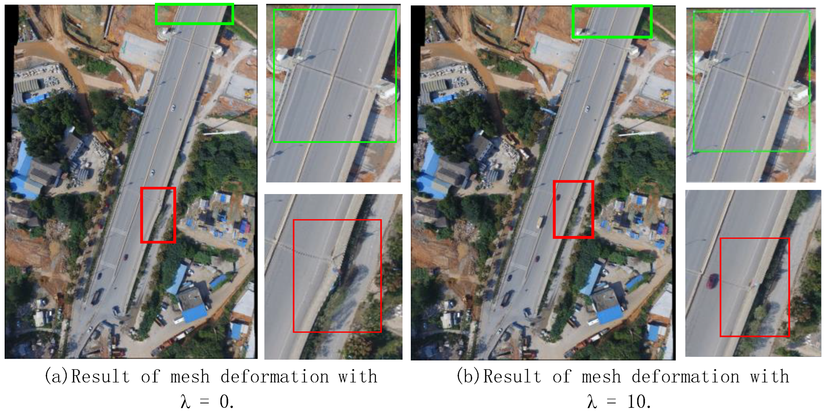
For the parameters setting, the grid size is set to 40 × 40, and the number of grids varies according to the size of image. We set $\sigma$ and $\gamma$$5,0.1$ for local mesh alignment. ${\lambda }_{pa},{\lambda }_{la},{\lambda }_l,{\lambda }_g,{\lambda }_b,{\lambda }_g$ are set to $3,10,10,1,10,10$ for energy minimization. There is no serious conflict between energy terms, so it can be solved stably. All codes run in MATLAB2019a (some algorithms are in C++) on a laptop with Inter i7 2.8 GHz CPU and 8 GB RAM. In the next sections, we will compare and analyze the stitching results of our proposed method with other methods based on alignment accuracy, structure preservation, quantitative evaluation of linear structure and time efficiency respectively.

Due to space constraints, some details in the stitching results cannot be well presented, so we uploaded the stitching results online. The stitching results can be seen and downloaded online at https://postimg.cc/gallery/0P0L5Zc (accessed on 1 March 2023).

3.1. Comparison of Alignment Accuracy

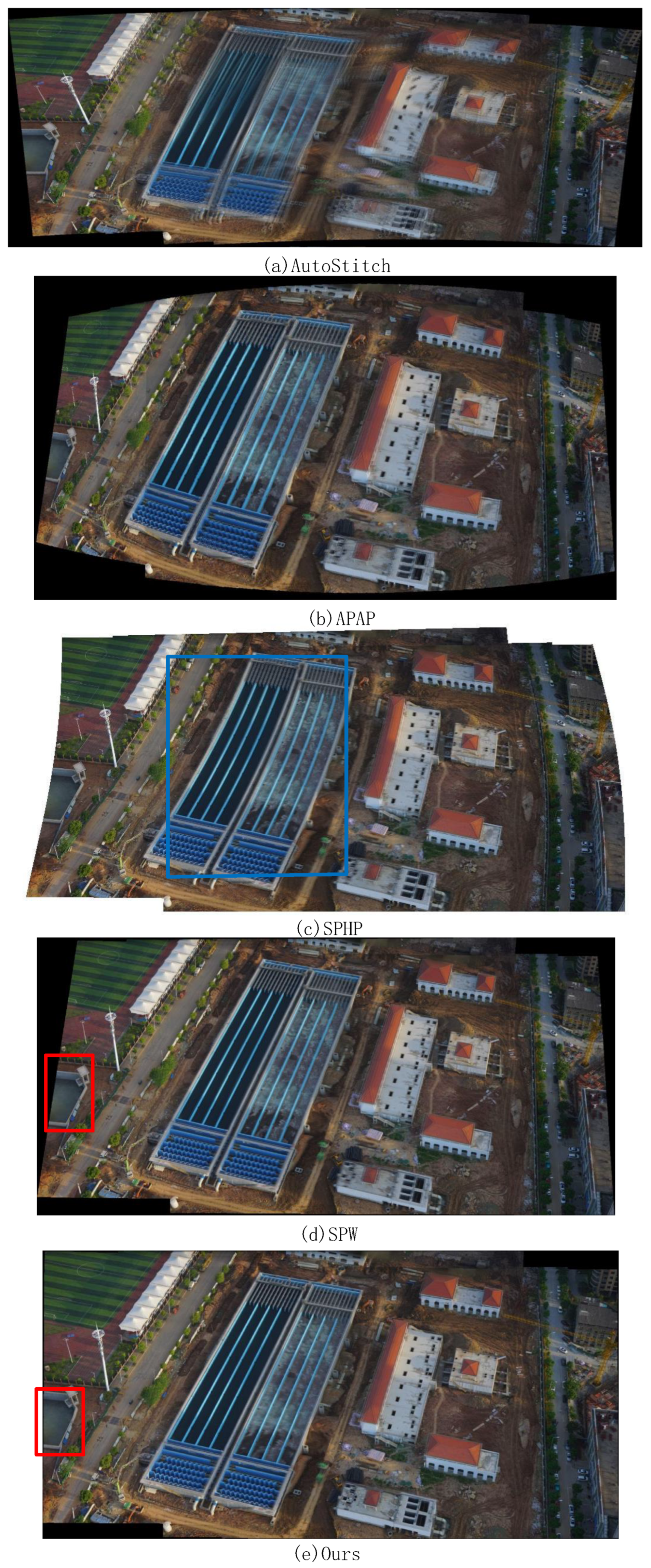
The alignment accuracy can be evaluated qualitatively and quantitatively. The qualitative evaluation of alignment accuracy can be understood as the degree of blurring and dislocation in overlapping areas. Figure 11 and Figure 12 show two groups of comparison results with AutoStitch [22], APAP [24], SPHP [27], SPW [36] and our proposed method to verify the alignment performance of our proposed method. To better compare the alignment of overlapping areas, we avoid post-processing and use linear blending to blend warping images.

As for quantitative evaluation of point alignment, we use root mean square error (RMSE) and mean square absolute error (MAE) as quantitative evaluation indicators which can be defined as:

$$\begin{array}{c}\hfill \mathrm{RMSE}=\sqrt{\frac{1}{N}\sum _{i=1}^N{\left|\left|\phi \left(p_i\right)-\phi \left(q_i\right)\right|\right|}^2}\end{array}$$

(24)

$$\begin{array}{c}\hfill \mathrm{MAE}=\frac{1}{N}\sum _{i=1}^N\sqrt{{\left|\left|\phi \left(p_i\right)-\phi \left(q_i\right)\right|\right|}^2}\end{array}$$

(25)

where N is the total number of matching points; $\phi$ is the align model that projects points onto the reference image plane, if the point is on the reference image, $\phi \left(p\right)=p$; $p_i$ and $q_i$ is a pair of point correspondence.

The smaller the values, the better the performance, and the units of RMSE and MAE are pixels. We compare our proposed method with other methods including global homography, APAP [24], SPHP [27] and SPW [36] (The AutoStitch [22] provided by the authors is a software, so we cannot calculate its RMSE and MAE).

Figure 11 shows a set of stitching results, including roads and building complexes. The content in the red box emphasizes the performance of line alignment, while the content in the blue box emphasizes the point alignment. Global transformation such as AutoStitch cannot align overlapping regions well because the global homography is not flexible enough which is only applicable to near planar scenes. The building complex and line segments in overlapping areas have obvious dislocations and ghosts as shown in Figure 11a. APAP and SPHP can reduce alignment error by constructing local homography warps. However they cannot handle the dislocations of line segments and there are still ghosts and dislocations. We mark it with red and blue boxes in Figure 11b,c. SPW can solve alignment and distortion problems through mesh-based warp combined with line feature, but there is still misalignment in line segments and buildings as shown in Figure 11d. Our method can better align line segments because we introduce global collinear structure which can impose more accurate constraints on matching line segments. Our method also has smaller ghosts in a building complex of overlapping areas than other methods in Figure 11e.

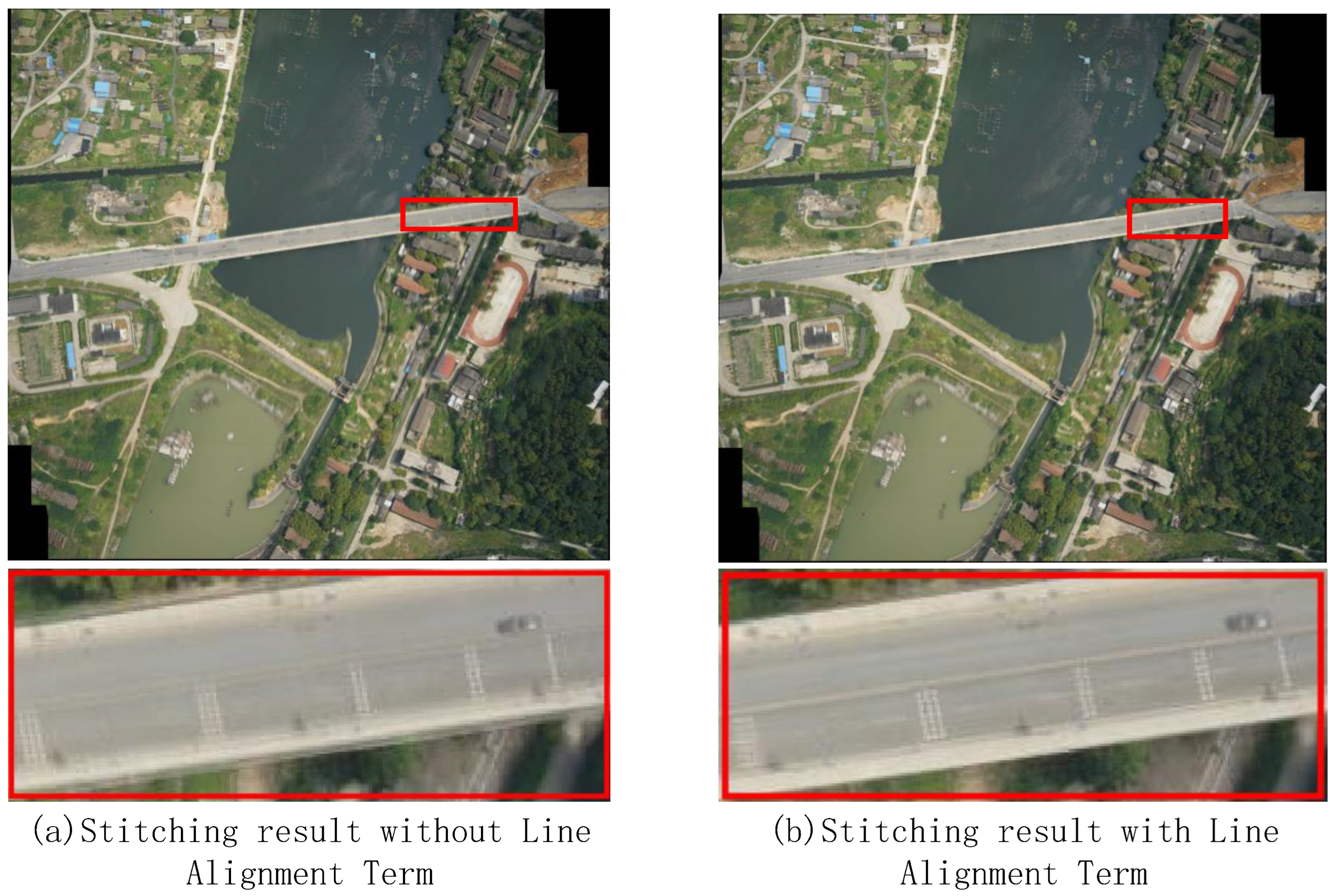
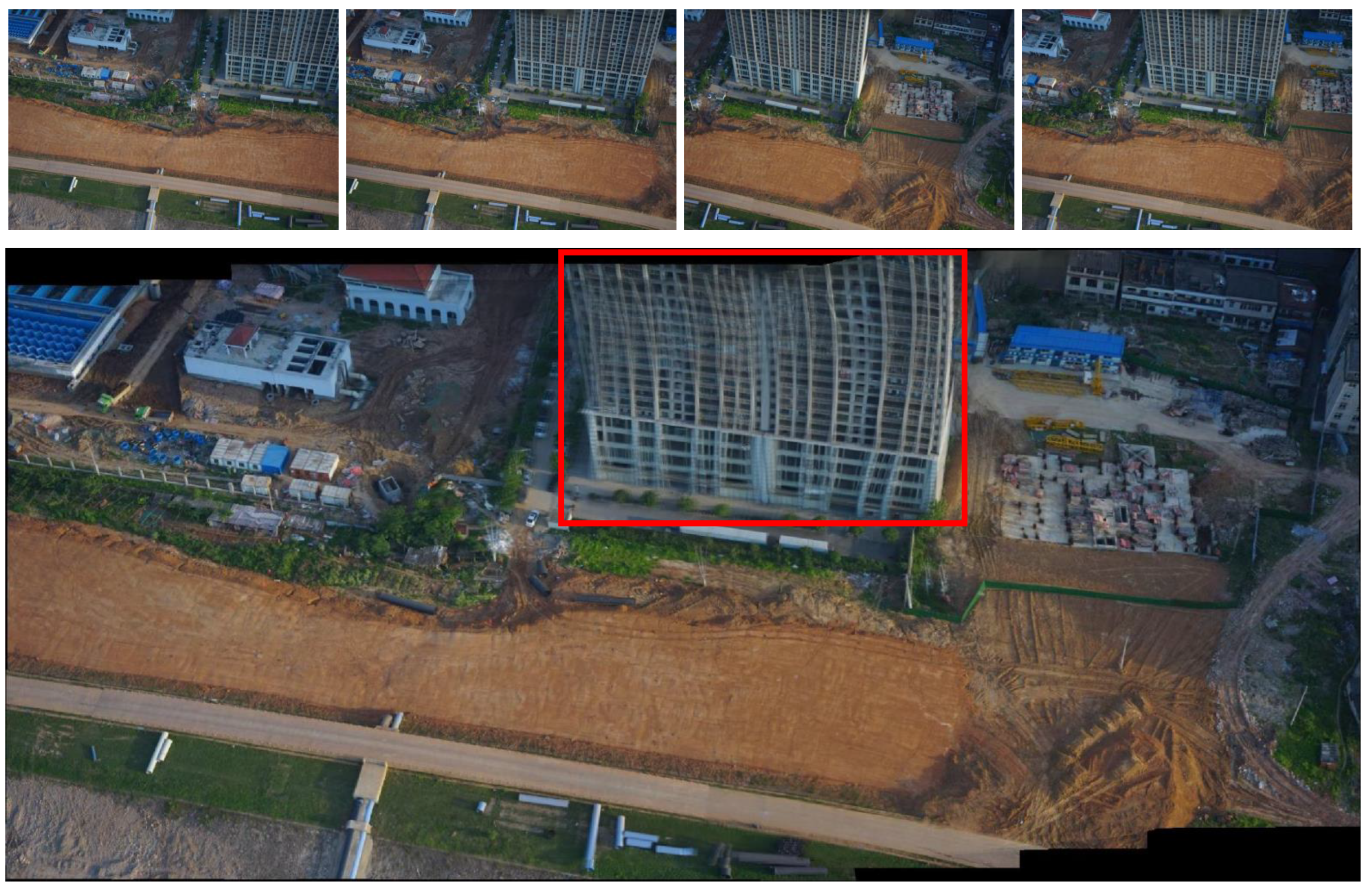
Figure 12 shows another set of stitching results run through by a highway which can more clearly evaluate the performance of line alignment. AutoStitch, APAP, and SPHP cannot align line segments because they construct transformations (global or local) only based on point correspondence as shown in Figure 12a–c. SPW introduces line features and constructs energy functions based on dual features to prevent distortion of line segments and align matching line segments, but there is still misalignment between line segments in the red box in Figure 12d. The stitching results of our proposed method show almost no misalignment between matching line segments, and the ghosts between the building clusters are also smaller than other methods, as shown in Figure 12e.

Table 1. Comparison of alignment accuracy of different methods.

Datasets	Index	Before BA	After BA	APAP	SPHP	SPW	Ours
Data1	RMSE	8.5970	8.5933	6.0377	6.1574	6.0629	5.5972
Figure 13	MAE	3.3678	3.3686	3.2540	3.3420	3.3219	1.9391
Data2	RMSE	2.1240	2.1266	5.6750	5.6471	5.5147	1.7673
Figure 14	MAE	1.7257	1.7159	3.1976	3.4526	2.4515	1.3377
Data3	RMSE	4.0980	3.9971	4.1204	4.0186	3.6397	2.2896
	MAE	3.2134	2.9791	2.7285	2.5143	2.0645	1.4130
Data4	RMSE	7.4242	7.3383	5.6271	6.0172	5.4306	5.0339
Figure 12	MAE	4.0264	3.8054	3.9023	3.8165	3.5662	2.4688
Data5	RMSE	4.7913	4.6823	5.0560	4.7183	3.6900	1.7478
	MAE	3.6084	3.4613	3.2635	3.1875	2.3887	1.3112
Data6	RMSE	5.1488	5.0816	5.0320	5.1276	4.4688	2.6228
Figure 11	MAE	4.1076	4.0113	3.8081	3.7981	3.0834	1.9424
Data7	RMSE	4.1558	4.0995	4.7475	4.5742	3.9555	1.6042
Figure 7	MAE	3.3132	3.1776	2.9829	2.8156	1.9492	1.1854
Data8	RMSE	3.9221	3.9119	4.7154	4.5639	4.3168	2.3277
	MAE	3.1401	3.1309	3.0517	2.9813	2.7530	1.8276

shows the RMSE and MAE values of eight different datasets. Global homography has a higher alignment error than other methods. Bundle adjustment can reduce transfer errors, but alignment issues still exist due to insufficient flexibility of the global homography. APAP can effectively improve alignment accuracy by constructing a local alignment model. SPHP constructs a shape-preserving half-projective warp to mitigate the perspective distortion in non overlapping areas, but cannot align images better. SPW and our method can reduce alignment error further by constructing energy functions based on mesh optimization and our method has lower RMSE and MAE because we apply a higher weight to the point alignment which is consistent with the effects shown in figures.

3.2. Comparison of Structure Preservation

Figure 13 and Figure 14 show two groups of stitching results of different methods and we evaluate the quality of stitching results in terms of structure preservation.

Figure 13 shows the playground dataset. The global homography can protect the linear structure well, but it suffers from alignment issues; there are very serious ghosts and dislocations, we mark them with a red box in Figure 13a. APAP can alleviate alignment problems; the playground is accurately aligned, which can be seen in Figure 13b. However, it suffers from distortions in non-overlapping areas especially in marginal areas and the line segments are slightly bent, we mark it with a green line. SPHP can alleviate the distortion of the non-overlapping area by introducing similarity transformation, but the linear structure is bent during warping and the shape of the playground is distorted as shown in Figure 13c. SPW and our proposed method can effectively solve alignment and distortion problems by a mesh-based warp. The stitching result of ours is more natural-looking because we impose rectangular constraint on the boundary of the stitching result, as shown in Figure 13d,e.

Figure 14 shows the stitching result of another dataset which contains many linear structures. The result of AutoStitch has obvious ghosts in Figure 14a. APAP can improve alignment accuracy but there are distortions in marginal areas. SPHP cannot protect the linear structure, the line segments are bent seriously, and we mark it with a blue box in Figure 14c. SPW can preserve linear structure well using the mesh-based warp based on double features as shown in Figure 14d. In addition to preserving linear structures, we also impose constraints on the boundary to obtain stitching results with regular boundary. The content of the boundary is preserved well during the optimization process which can be seen in Figure 14e.

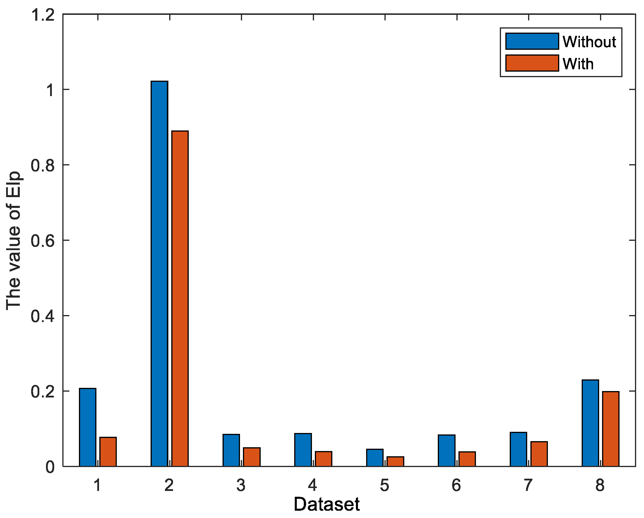
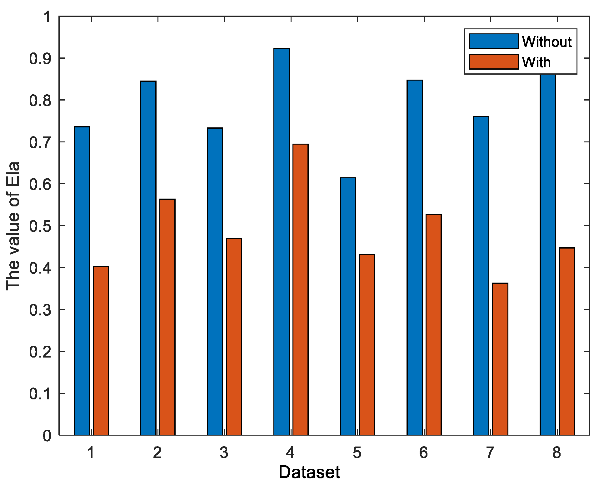
3.3. Quantitative Comparison of Linear Structure

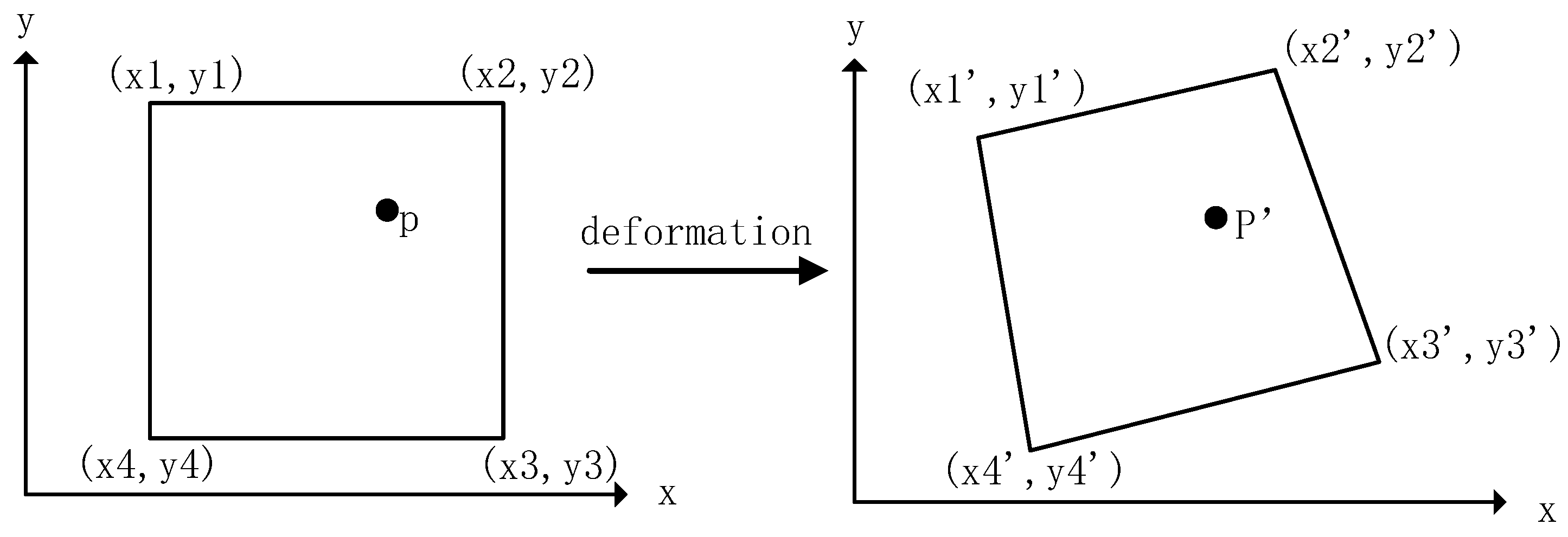
In order to quantify the performance of line alignment and line preservation of our proposed method, we design a new evaluation method. The evaluation method is based on the distance from point to line, and includes two parts: the line alignment indicator $E_{la}$ and line preservation indicator $E_{lp}$.

Given a set of line segments ${\left\{l_i\right\}}_{i=1}^K$ detected by LSD [41], where K is the number of line segments. We first remove the shorter line segments, then uniformly sample them ${\left\{p_j^i\right\}}_{j=1}^{J_i}$. The sample points may not be in a straight line after warping (see Figure 15a). We use the distance from the sample points to the straight line as the indicator of point deviation from the straight line. Thus the error term $E_{lp}$ can be defined as:

$$\begin{array}{c}\hfill E_{lp}=\frac{1}{K}\sum _{i=1}^K\frac{1}{J_i}\sum _{j=1}^{J_i}dis\left(\phi \left(p_j^i\right),\phi \left(l_i\right)\right)\end{array}$$

(26)

where $\phi \left(l_i\right)$ is the i-th line segment projected on the reference image plane which is obtained by projecting the start point and end point of line segment onto the reference image plane, dis is the distance from point $p_j^i$ to the line $\phi \left(l_i\right)$, which is defined as:

$$\begin{array}{c}\hfill dis\left(p,l\right)=\left|\frac{ax+by+c}{\sqrt{a^2+b^2}}\right|\end{array}$$

(27)

where $\left(x,y\right)$ is the coordinates of point p, $\left(a,b,c\right)$ are the parameters of the line segment l.

Given a set of line segment correspondences ${\left\{l_i,l_i^{\prime }\right\}}_{i=1}^M$, where M is the number of matching line segments, then uniformly sample these line segments ${\left\{p_j^i\right\}}_{j=1}^{J_i}\in l_i$, ${\left\{q_j^{i^{\prime }}\right\}}_{j=1}^{J_i^{\prime }}\in l_i^{\prime }$. For the sample points on $l_i$ and $l_i^{\prime }$, we calculate the distance from the sample points $\phi \left(p_j^i\right)$, $\phi \left(q_j^i\right)$ to the line $\phi \left(l_i^{\prime }\right)$ and $\phi \left(l_i\right)$, respectively, then average them (see Figure 15b). Thus the error term $E_{la}$ can be defined as:

$$\begin{array}{cc}\hfill E_{la}& =\frac{1}{2M}\sum _{i=1}^M\frac{1}{J_i}\sum _{j=1}^{J_i}dis\left(\phi \left(p_j^i\right),\phi \left(l_i^{\prime }\right)\right)\hfill \\ \hfill & +\frac{1}{2M}\sum _{i=1}^M\frac{1}{J_i^{\prime }}\sum _{j=1}^{J_i^{\prime }}dis\left(\phi \left(q_j^{i^{\prime }}\right),\phi \left(l_i\right)\right)\hfill \end{array}$$

(28)

These two indicators reflect the distance from the sampling points to the straight line, thus their units are pixels.

Table 2. Quantitative comparison of line alignment and line preservation.

Datasets	Line Preservation		Line Alignment
	SPW	Ours	SPW	Ours
Data1	0.0528	0.0771	0.7009	0.4026
Data2	0.9668	0.8897	0.8644	0.5631
Data3	0.0526	0.0493	0.7470	0.4691
Data4	0.0220	0.0388	0.7049	0.6947
Data5	0.0194	0.0251	0.8841	0.4308
Data6	0.0378	0.0384	1.0798	0.5268
Data7	0.0670	0.0652	0.7157	0.3625
Data8	0.1682	0.1986	0.8950	0.4466

shows a set of quantitative assessments of $E_{la}$ and $E_{lp}$ compared with SPW which only constrains local line segments. For fair comparison, the line segments data used for testing is the same with SPW.

Table 2 shows that our proposed method can align line segments better than SPW because we impose stronger constraints on the matching line segments which is consistent with the effects shown in figures and the ability to maintain line segments is comparable to SPW as shown in Table 2. The $E_{lp}$ is larger in some datasets than SPW, probably because the line segments are slightly bent when constraining the boundary, but this tiny error is not noticeable on the stitching results.

3.4. Comparison of Time Efficiency

In this part, we quantitatively compare the time spent of our proposed method with APAP, SPHP, and SPW on different datasets. All the methods are running in MATLAB2019a with the same environment.

Table 3. Comparison of elapsed time of different methods.

Methods	Index	APAP	SPHP	SPW	Ours
Data1	time(s)	20.694	8.352	6.750	7.283
Data2	time(s)	11.197	5.5250	4.8120	4.682
Data3	time(s)	12.325	7.815	5.782	5.378
Data4	time(s)	10.276	8.235	4.177	3.461
Data5	time(s)	31.764	20.673	15.685	14.205
Data6	time(s)	34.624	30.862	21.155	16.337
Data7	time(s)	31.613	17.746	14.039	13.098
Data8	time(s)	25.737	15.101	11.220	9.965

shows the elapsed time of different methods for stitching images. All the methods are running in MATLAB. The elapsed time of our method includes bundle adjustment, local mesh alignment, line-segments detection, energy function construction, iterative solution, texture mapping, and linear blend. The time for feature detection and matching is not included. The elapsed time calculated from other methods is the same.

As shown in the Table 3, SPW and our method are comparative because they are both based on mesh optimization and do not have additional parameter calculations. Our method takes less time because we do not add the line feature into bundle adjustment and our energy terms spend less time than SPW. APAP and SPHP spend more time because they both need to calculate many local homography warps and APAP takes a lot of time to perform bundle adjustment for each mesh.

3.5. Failure Cases and Discussion

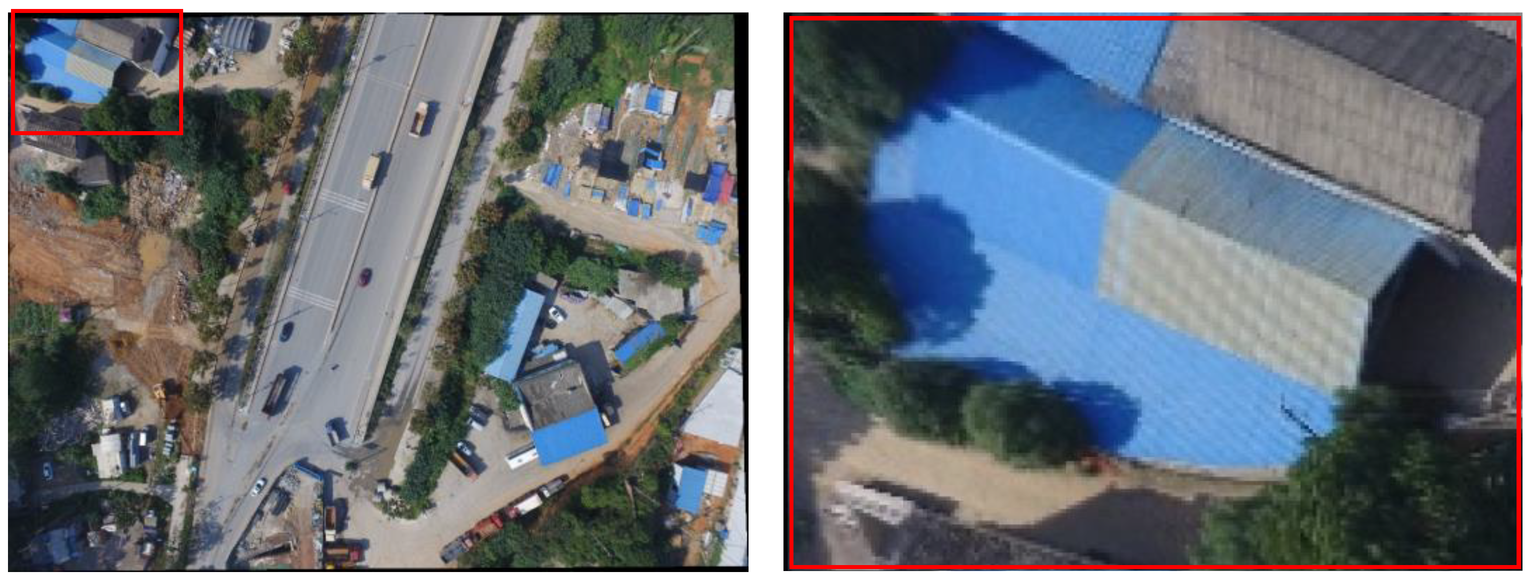
The experimental results show that our method can achieve accurate alignment, structure preservation, and obtain more natural panorama, but there are still some limitations. Our proposed method may fail if the dominant plane cannot well represent the perspective transformation between images. This usually happens when the captured pictures contain more than one main plane.

Figure 16 shows a set of failure cases. In this case, the input images contain two planes, the ground plane and the tall buildings plane. We are unable to precisely align the tall building because the dominant plane cannot well represent the perspective transformation between tall buildings in different input images. In addition the line preservation term may not work properly in this case because the calculated global homography cannot provide proper perspective transformation. In future work, we may focus on stitching images with a large parallax, and on increasing the speed of stitching.

4. Conclusions

In this paper, a novel effective and flexible mesh-based UAV image-stitching strategy is proposed to obtain a natural-looking panorama. We consider improving alignment accuracy from both global and local aspects. First, global bundle adjustment is adopted to obtain more accurate global homography, then mesh-based local bundle adjustment is incorporated into the minimum energy function framework to reduce parallax error further. Distortions of salient structure may occur during optimization which will affect the stitching quality seriously. Considering that the human eye is sensitive to lines, we attempt to introduce line features into the framework and extend it to the global collinear structure. Then, energy functions guided by the global collinear structure are designed to better align matching-line segments and preserve the linear structure. As an important complement to our proposed method, the regular boundary constraint combined with the shape preserving transform is introduced to obtain more natural-looking stitching results with a rectangular boundary. Two new quantitative indicators of linear structure are also developed to measure the preservation and alignment of linear structure for image stitching. Experimental results show that our method can better align images, preserve a salient structure, and obtain more natural results.

Although our method can obtain more accurate stitching results, there are still some issues to be resolved. For example, the computational complexity of our proposed method gradually increases as the number and resolution of images increase, making it impossible to achieve real-time stitching. In addition, oblique images contain more information, but the distortion also increases, and the stitching of oblique images is still a challenge. Next, we will focus on studying how to reduce the cost of time while improving the quality of stitching, as well as how to stitch oblique images.

References

1. Bryson, M.; Reid, A.; Ramos, F.; Sukkarieh, S. Airborne vision-based mapping and classification of large farmland environments. J. Field Robot. 2010, 27, 632–655. [Google Scholar] [CrossRef]
2. Yahyanejad, S.; Wischounig-Strucl, D.; Quaritsch, M.; Rinner, B. Incremental mosaicking of images from autonomous, small-scale uavs. In Proceedings of the 2010 7th IEEE International Conference on Advanced Video and Signal Based Surveillance, Boston, MA, USA, 29 August–1 September 2010; pp. 329–336. [Google Scholar]
3. Ezequiel, C.A.F.; Cua, M.; Libatique, N.C.; Tangonan, G.L.; Alampay, R.; Labuguen, R.T.; Favila, C.M.; Honrado, J.L.E.; Canos, V.; Devaney, C.; et al. UAV aerial imaging applications for post-disaster assessment, environmental management and infrastructure development. In Proceedings of the 2014 International Conference on Unmanned Aircraft Systems (ICUAS), Orlando, FL, USA, 27–30 May 2014; pp. 274–283. [Google Scholar]
4. Shao, R.; Du, C.; Chen, H.; Li, J. Fast anchor point matching for emergency UAV image stitching using position and pose information. Sensors 2020, 20, 2007. [Google Scholar] [CrossRef] [Green Version]
5. Bu, S.; Zhao, Y.; Wan, G.; Liu, Z. Map2DFusion: Real-time incremental UAV image mosaicing based on monocular SLAM. In Proceedings of the 2016 IEEE/RSJ International Conference on Intelligent Robots and Systems (IROS), Daejeon, Republic of Korea, 9–14 October 2016; pp. 4564–4571. [Google Scholar]
6. Xu, Y.; Ou, J.; He, H.; Zhang, X.; Mills, J. Mosaicking of unmanned aerial vehicle imagery in the absence of camera poses. Remote Sens. 2016, 8, 204. [Google Scholar] [CrossRef]
7. Yuan, Y.; Fang, F.; Zhang, G. Superpixel-based seamless image stitching for UAV images. IEEE Trans. Geosci. Remote Sens. 2020, 59, 1565–1576. [Google Scholar] [CrossRef]
8. Wan, Q.; Chen, J.; Luo, L.; Gong, W.; Wei, L. Drone Image Stitching Using Local Mesh-Based Bundle Adjustment and Shape-Preserving Transform. IEEE Trans. Geosci. Remote Sens. 2020, 59, 7027–7037. [Google Scholar] [CrossRef]
9. Guo, D.; Chen, J.; Luo, L.; Gong, W.; Wei, L. UAV Image Stitching Using Shape-Preserving Warp Combined with Global Alignment. IEEE Geosci. Remote Sens. Lett. 2021, 19, 8016005. [Google Scholar] [CrossRef]
10. Jiang, X.; Ma, J.; Xiao, G.; Shao, Z.; Guo, X. A review of multimodal image matching: Methods and applications. Inf. Fusion 2021, 73, 22–71. [Google Scholar] [CrossRef]
11. Lowe, D.G. Distinctive image features from scale-invariant keypoints. Int. J. Comput. Vis. 2004, 60, 91–110. [Google Scholar] [CrossRef]
12. Bay, H.; Tuytelaars, T.; Gool, L.V. Surf: Speeded up robust features. Lect. Notes Comput. Sci. 2006, 3951, 404–417. [Google Scholar]
13. Rublee, E.; Rabaud, V.; Konolige, K.; Bradski, G. ORB: An efficient alternative to SIFT or SURF. In Proceedings of the 2011 International Conference on Computer Vision, Barcelona, Spain, 6–13 November 2011; pp. 2564–2571. [Google Scholar]
14. Fischler, M.A.; Bolles, R.C. Random sample consensus: A paradigm for model fitting with applications to image analysis and automated cartography. Commun. ACM 1981, 24, 381–395. [Google Scholar] [CrossRef]
15. Torr, P.H.; Zisserman, A. MLESAC: A new robust estimator with application to estimating image geometry. Comput. Vis. Image Underst. 2000, 78, 138–156. [Google Scholar] [CrossRef] [Green Version]
16. Raguram, R.; Chum, O.; Pollefeys, M.; Matas, J.; Frahm, J.M. USAC: A universal framework for random sample consensus. IEEE Trans. Pattern Anal. Mach. Intell. 2012, 35, 2022–2038. [Google Scholar] [CrossRef]
17. Ma, J.; Zhao, J.; Jiang, J.; Zhou, H.; Guo, X. Locality preserving matching. Int. J. Comput. Vis. 2019, 127, 512–531. [Google Scholar] [CrossRef]
18. Jiang, X.; Xia, Y.; Zhang, X.P.; Ma, J. Robust image matching via local graph structure consensus. Pattern Recognit. 2022, 126, 108588. [Google Scholar] [CrossRef]
19. Yi, K.M.; Trulls, E.; Ono, Y.; Lepetit, V.; Salzmann, M.; Fua, P. Learning to find good correspondences. In Proceedings of the IEEE Conference on Computer Vision and Pattern Recognition, Salt Lake City, UT, USA, 18–23 June 2018; pp. 2666–2674. [Google Scholar]
20. Ma, J.; Jiang, X.; Jiang, J.; Zhao, J.; Guo, X. LMR: Learning a two-class classifier for mismatch removal. IEEE Trans. Image Process. 2019, 28, 4045–4059. [Google Scholar] [CrossRef] [PubMed]
21. Szeliski, R. Image alignment and stitching: A tutorial. Found. Trends Comput. Graph. Vis. 2007, 2, 1–104. [Google Scholar] [CrossRef]
22. Brown, M.; Lowe, D.G. Automatic panoramic image stitching using invariant features. Int. J. Comput. Vis. 2007, 74, 59–73. [Google Scholar] [CrossRef] [Green Version]
23. Lin, W.Y.; Liu, S.; Matsushita, Y.; Ng, T.T.; Cheong, L.F. Smoothly varying affine stitching. In Proceedings of the CVPR 2011, Colorado Springs, CO, USA, 20–25 June 2011; pp. 345–352. [Google Scholar]
24. Zaragoza, J.; Chin, T.J.; Brown, M.S.; Suter, D. As-projective-as-possible image stitching with moving DLT. In Proceedings of the IEEE Conference on Computer Vision and Pattern Recognition, Portland, OR, USA, 23–28 June 2013; pp. 2339–2346. [Google Scholar]
25. Zhang, F.; Liu, F. Parallax-tolerant image stitching. In Proceedings of the IEEE Conference on Computer Vision and Pattern Recognition, Columbus, OH, USA, 23–28 June 2014; pp. 3262–3269. [Google Scholar]
26. Lin, K.; Jiang, N.; Cheong, L.F.; Do, M.; Lu, J. Seagull: Seam-guided local alignment for parallax-tolerant image stitching. In Proceedings of the European Conference on Computer Vision, Amsterdam, The Netherlands, 11–14 October 2016; Springer: Berlin/Heidelberg, Germany, 2016; pp. 370–385. [Google Scholar]
27. Chang, C.H.; Sato, Y.; Chuang, Y.Y. Shape-preserving half-projective warps for image stitching. In Proceedings of the IEEE Conference on Computer Vision and Pattern Recognition, Columbus, OH, USA, 23–28 June 2014; pp. 3254–3261. [Google Scholar]
28. Lin, C.C.; Pankanti, S.U.; Natesan Ramamurthy, K.; Aravkin, A.Y. Adaptive as-natural-as-possible image stitching. In Proceedings of the IEEE Conference on Computer Vision and Pattern Recognition, Boston, MA, USA, 7–12 June 2015; pp. 1155–1163. [Google Scholar]
29. Chen, Y.S.; Chuang, Y.Y. Natural image stitching with the global similarity prior. In Proceedings of the European Conference on Computer Vision, Amsterdam, The Netherlands, 11–14 October 2016; Springer: Berlin/Heidelberg, Germany, 2016; pp. 186–201. [Google Scholar]
30. Li, N.; Xu, Y.; Wang, C. Quasi-homography warps in image stitching. IEEE Trans. Multimed. 2017, 20, 1365–1375. [Google Scholar] [CrossRef] [Green Version]
31. Li, J.; Wang, Z.; Lai, S.; Zhai, Y.; Zhang, M. Parallax-tolerant image stitching based on robust elastic warping. IEEE Trans. Multimed. 2017, 20, 1672–1687. [Google Scholar] [CrossRef]
32. Joo, K.; Kim, N.; Oh, T.H.; Kweon, I.S. Line meets as-projective-as-possible image stitching with moving DLT. In Proceedings of the 2015 IEEE International Conference on Image Processing (ICIP), Quebec City, QC, Canada, 27–30 September 2015; pp. 1175–1179. [Google Scholar]
33. Chang, C.H.; Chuang, Y.Y. A line-structure-preserving approach to image resizing. In Proceedings of the 2012 IEEE Conference on Computer Vision and Pattern Recognition, Providence, RI, USA, 16–21 June 2012; pp. 1075–1082. [Google Scholar]
34. Zhang, G.; He, Y.; Chen, W.; Jia, J.; Bao, H. Multi-viewpoint panorama construction with wide-baseline images. IEEE Trans. Image Process. 2016, 25, 3099–3111. [Google Scholar] [CrossRef]
35. Xiang, T.Z.; Xia, G.S.; Bai, X.; Zhang, L. Image stitching by line-guided local warping with global similarity constraint. Pattern Recognit. 2018, 83, 481–497. [Google Scholar] [CrossRef] [Green Version]
36. Liao, T.; Li, N. Single-perspective warps in natural image stitching. IEEE Trans. Image Process. 2019, 29, 724–735. [Google Scholar] [CrossRef] [Green Version]
37. Jia, Q.; Li, Z.; Fan, X.; Zhao, H.; Teng, S.; Ye, X.; Latecki, L.J. Leveraging line-point consistence to preserve structures for wide parallax image stitching. In Proceedings of the IEEE/CVF Conference on Computer Vision and Pattern Recognition, Nashville, TN, USA, 20–25 June 2021; pp. 12186–12195. [Google Scholar]
38. He, K.; Chang, H.; Sun, J. Rectangling panoramic images via warping. ACM Trans. Graph. (TOG) 2013, 32, 1–10. [Google Scholar] [CrossRef]
39. Zhang, Y.; Lai, Y.K.; Zhang, F.L. Content-preserving image stitching with piecewise rectangular boundary constraints. IEEE Trans. Vis. Comput. Graph. 2020, 27, 3198–3212. [Google Scholar] [CrossRef] [PubMed]
40. Nie, L.; Lin, C.; Liao, K.; Liu, S.; Zhao, Y. Deep Rectangling for Image Stitching: A Learning Baseline. In Proceedings of the IEEE/CVF Conference on Computer Vision and Pattern Recognition, New Orleans, LA, USA, 8–24 June 2022; pp. 5740–5748. [Google Scholar]
41. Von Gioi, R.G.; Jakubowicz, J.; Morel, J.M.; Randall, G. LSD: A fast line segment detector with a false detection control. IEEE Trans. Pattern Anal. Mach. Intell. 2008, 32, 722–732. [Google Scholar] [CrossRef]
42. Heckbert, P.S. Fundamentals of Texture Mapping and Image Warping. Master’s Thesis, University of California, Berkeley, CA, USA, 1989. [Google Scholar]
43. Hejazifar, H.; Khotanlou, H. Fast and robust seam estimation to seamless image stitching. Signal Image Video Process. 2018, 12, 885–893. [Google Scholar] [CrossRef]
44. Jia, Q.; Gao, X.; Fan, X.; Luo, Z.; Li, H.; Chen, Z. Novel coplanar line-points invariants for robust line matching across views. In Proceedings of the European Conference on Computer Vision, Amsterdam, The Netherlands, 11–14 October 2016; Springer: Berlin/Heidelberg, Germany, 2016; pp. 599–611. [Google Scholar]
45. Martinez, F.; Ogayar, C.; Jiménez, J.R.; Rueda, A.J. A simple algorithm for Boolean operations on polygons. Adv. Eng. Softw. 2013, 64, 11–19. [Google Scholar] [CrossRef]
46. Zhang, G.X.; Cheng, M.M.; Hu, S.M.; Martin, R.R. A shape-preserving approach to image resizing. In Computer Graphics Forum; Wiley Online Library: Oxford, UK, 2009; Volume 28, pp. 1897–1906. [Google Scholar]
47. Paige, C.C.; Saunders, M.A. LSQR: An algorithm for sparse linear equations and sparse least squares. ACM Trans. Math. Softw. (TOMS) 1982, 8, 43–71. [Google Scholar] [CrossRef] [Green Version]
48. Triggs, B.; McLauchlan, P.F.; Hartley, R.I.; Fitzgibbon, A.W. Bundle adjustment—A modern synthesis. In Proceedings of the International Workshop on Vision Algorithms, Corfu, Greece, 21–22 September 1999; Springer: Berlin/Heidelberg, Germany, 1999; pp. 298–372. [Google Scholar]
49. Agarwal, S.; Mierle, K. Ceres Solver; Google Inc.: Mountain View, CA, USA, 2012. [Google Scholar]
50. Vedaldi, A.; Fulkerson, B. VLFeat: An open and portable library of computer vision algorithms. In Proceedings of the 18th ACM international conference on Multimedia, Firenze, Italy, 25–29 October 2010; pp. 1469–1472. [Google Scholar]
Figure 1. Flowchart of our proposed method.
Drones 07 00230 g001
Figure 2. Illustration of detected point (blue) and line (red) feature.
Drones 07 00230 g002
Figure 3. Point p and the four vertices of mesh before and after deformation.
Drones 07 00230 g003
Figure 4. Illustration of bending of line segments due to the local mesh alignment. (Left) Warping result of local mesh alignment of one image. (Right) The enlarged area of the red box on the left image which explains the bending effect on line segments of local mesh alignment.
Drones 07 00230 g004
Figure 5. Comparison of stitching results with and without salient structure preservation term. (a) The stitching result of mesh optimization without salient line preservation term. (b) The stitching results of mesh optimization with the λ l = 10 . The red box indicates the bending of line segments caused by point alignment, the green box indicates the bending of line segments caused by the rectangle boundary constraint term.
Drones 07 00230 g005
Figure 6. Quantitative comparison of different datasets with and without salient structure preservation term.
Drones 07 00230 g006
Figure 7. Comparison of stitching result with and without line alignment term. (a) The stitching result without line alignment term. (b) The stitching result with the λ l a = 10 . For better comparison, we enlarge the contents in the red box by the same factor, and put them below the stitching results.
Drones 07 00230 g007
Figure 8. Quantitative comparison of stitching result with and without line alignment term.
Drones 07 00230 g008
Figure 9. Comparison of stitching results with and without shape preservation term and rectangle boundary constraint term. The content in the blue box is enlarged by the same factor and placed below the stitching results.
Drones 07 00230 g009
Figure 10. Illustration of matching line segments: the red line segment is a group of matching line segment between target image 1 and target image 2, the blue one is a group of matching line segment between target image 1 and reference image, and the green line is the extended line segment of matching line segment. The red line segment and the blue line segment in target image 1 have the same extended line segment. Thus, the red line segment in target image 2 and the blue line segment in reference image can be considered as a set of matching line segments.
Drones 07 00230 g010
Figure 11. Qualitative comparison of alignment accuracy. From top to bottom, the first row is the input image, the others are the stitching results of (a) AutoStitch [22], (b) APAP [24], (c) SPHP [27], (d) SPW [36] and (e) our proposed method, respectively. For clearer comparison, we enlarge some areas and place them on the right side of the stitching results. The contents in the box are magnified by the same factor. The red box highlights the line alignment, and the blue box highlights the point alignment.
Drones 07 00230 g011
Figure 12. Qualitative comparison of alignment accuracy. From top to bottom, the first row is the input image, the others are the stitching results of (a) AutoStitch [22], (b) APAP [24], (c) SPHP [27], (d) SPW [36] and (e) our proposed method, respectively. For clearer comparison, we enlarge some areas and place them on the right side of the stitching results. The red box highlights the line alignment, and the blue box highlights the point alignment.
Drones 07 00230 g012
Figure 13. Qualitative comparison of structure preservation. From top to bottom are the input images, stitching results of (a) AutoStitch [22], (b) APAP [24], (c) SPHP [27], (d) SPW [36] and (e) our proposed method, respectively. For clearer comparison, we enlarge some areas and place them on the left side of the stitching results. The blue box and the red box highlight the alignment, and the green line and the yellow line on the stitching result highlight the preservation of alogrithm to linear structure.
Drones 07 00230 g013
Figure 14. Qualitative comparison of structure preservation. From top to bottom are the input images, stitching results of (a) AutoStitch [22], (b) APAP [24], (c) SPHP [27], (d) SPW [36], and (e) our proposed method respectively.
Drones 07 00230 g014
Figure 15. Quantitative evaluation methods of linear structure: (a) line preservation indicator: the blue points are the start and end point of line segment. The red points are the sampling points of the line segment. (b) line alignment indicator: The red points are the sampling points of line segment l, the green points are the sampling points of line segment l , l and l are a pair of matching line segments between target image 1 and target image 2. φ l is the line segment l projected on the reference image plane.
Drones 07 00230 g015
Figure 16. The failure case happens when the dominant plane cannot well represent the perspective transformation between images. The red box hignlights the misalignments.
Drones 07 00230 g016