Robust Planning System for Fast Autonomous Flight in Complex Unknown Environment Using Sparse Directed Frontier Points

Abstract

Path planning is one of the key parts of unmanned aerial vehicle (UAV) fast autonomous flight in cluttered environments. However, it remains a challenge to efficiently generate a high-quality trajectory for flight tasks with a high success rate. In this paper, a robust planning framework is proposed, which can stably support autonomous flight tasks in complex unknown environments with limited onboard computing resources. Firstly, we propose the directed frontier point information structure (DFP), which can roughly capture the frontier information of the explored environment. The planning direction of a local planner can be evaluated and rectified efficiently based on the DFP to avoid falling into traps with limited cost. Secondly, an adaptive fusion replanning method is designed to generate a high-quality trajectory efficiently by incorporating two optimization methods with different characteristics, which can both take advantage of different optimization methods while avoiding disadvantages as much as possible, but also adjust the focus of the optimization according to the actual situation to improve the success rate of the planning method. Finally, sufficient comparison and evaluation experiments in simulation environments are presented. Experimental results show the proposed method has better performance, especially in terms of adaptability and robustness, compared to typical and state-of-the-art methods in unknown complex scenarios. Moreover, the proposed system is integrated into a fully autonomous quadrotor, and the effectiveness of the proposed method is further evaluated by using the quadrotor in real-world environments.

1. Introduction

Unmanned aerial vehicles (UAVs) have been widely used in surveying and mapping [1,2,3,4,5,6], ecological monitoring [7], rescue [8], military, and other fields [9,10,11,12]. However, autonomy and intelligence are still lacking in these scenarios. As one of the key parts of UAV autonomous capability, the motion planning module plays an essential role in achieving full autonomy, which can provide a high-quality trajectory for UAV to generate safe and smooth motions [13,14,15].

Although many excellent motion planning algorithms have emerged in recent years, there are still some critical problems to be solved [16,17,18]. Firstly, most of the motion planning methods can only be used for fast obstacle avoidance of small obstacles. Once the work environment contains large obstacles, the methods will have a low success rate or even fail due to the lack of global information. Secondly, given limited time and onboard computing resources, there are few methods that can efficiently provide global-level guiding in real time. However, it is important to improve the stability and effectiveness of the planning methods in different flight tasks. Thirdly, few methods can efficiently generate a high-quality trajectory that satisfies various constraints in real time. Current motion planning methods use hard-constrained methods or soft-constrained methods to generate a trajectory. The former can generate a high-quality flight trajectory that strictly satisfies the constraints set in advance, but its planning efficiency is relatively low. The latter methods can generate a safe and smooth trajectory efficiently, but their optimization results do not strictly meet the various constraints. As a result, current motion planning methods are unable to meet the needs of real-time and high-quality planning tasks.

Motivated by the issues mentioned above, in this paper, we propose a robust online trajectory replanning system that can support fast autonomous flight in a complex, unknown environment. We innovatively propose a directed frontier point information structure (DFP) that can efficiently provide global guiding to evaluate and rectify the initial path generated by the local planner according to the essential frontier information (the boundary between reached and unreached areas) stored in DFP. The structure can be updated incrementally with limited costs when the new information is collected, so it can support high-frequency guiding to help the planner detour large obstacles or traps without a significant increase in computation and memory burden. Then, to generate a high-quality trajectory efficiently, a fusion trajectory replanning strategy is adopted, which consists of two different types of optimization methods. The hard-constrained method is used to generate a high-quality trajectory for a flight at a low frequency. The soft-constrained method is responsible for optimizing the local flight trajectory for fast obstacle avoidance when a newly discovered obstacle affects flight safety. Meanwhile, an adaptive optimization function is used to improve planning success rate and flight safety, which can adjust the focus of optimization by using different weight allocation according to the real-time flight environment.

We compare our method with three typical and state-of-the-art methods in three different simulation environments. The experimental results show that our proposed method not only improves the trajectory quality while maintaining efficient planning, but also significantly improves the adaptability and robustness of the planner to the environment with limited additional cost. In addition, we also verify the effectiveness of our method through onboard real-world experiments. The contributions of this paper are as follows:

• An incrementally updated DFP that can capture essential information from the entire unexplored space and provide global guiding efficiently to evaluate and rectify the direction of the local planner with limited costs in high frequency.
• A fusion replanning strategy, which incorporates two optimization methods with different characteristics to generate a high-quality trajectory efficiently. The method can achieve a balance between planning quality and efficiency by leveraging the advantages of different optimization methods through a reasonable replanning strategy.
• An adaptive optimization method that can adjust the focus of the optimization function by using different weight allocation according to the actual flight environment to improve planning stability.
• Sufficient quantitative comparison experiments are conducted in simulation. Meanwhile, real-world experiments are also carried out to validate our method in various environments.

The rest of the paper is organized as follows: Section 2 introduces the related work about motion planning. Section 3 describes the proposed robust planning system for fast flight by using DFP in detail. In Section 4, the experimental results of the proposed method are presented and analyzed. Finally, concluding remarks are presented in Section 5.

2. Related Work

The problem of motion planning has been studied by many scholars in recent years, and numerous methods from multiple angles have been proposed, mainly divided into the following two categories: hard-constrained methods and soft-constrained methods.

2.1. Hard-Constrained Methods

The method in [19] first adopted hard-constrained optimization to generate a minimum-snap trajectory by solving the quadratic programming (QP). Ref. [20] extended the work of [19], which used the close form to solve the minimum snap trajectories and designed a method to ensure the safety of the trajectories. To obtain a high-quality and safe trajectory, lots of methods [21,22,23] used a two-step pipeline for trajectory generation: safe flight corridor construction and convex optimization. Ref. [24] proposed a method to obtain a better flight trajectory by constructing a bigger safe flight corridor (SFC). Ref. [25] proposed an efficient method to track an agile target efficiently by optimizing the trajectory within a space flight corridor. Ref. [16] generated both a high-quality flight trajectory by SFC in free-known and unknown space and a safe replacement trajectory in free-known space. Meanwhile, they also proposed a method to generate a better time allocation for the trajectory. Ref. [26] proposed a flexible and efficient planning framework, which can reliably achieve high-efficiency, high-quality planning requirements by deforming and simplifying the planning problem.

2.2. Soft-Constrained Methods

Soft-constrained methods essentially constitute an approach that regards the trajectory generation problem as a non-linear optimization problem that takes smoothness, safety, and dynamic feasibility into account. Many studies have shown its superiority for fast and autonomous flight in unknown environments. Ref. [27] first introduced the Euclidean signed distance field (ESDF) and proposed a method to generate discrete-time trajectories by using covariant gradient descent. Ref. [28] proposed the stochastic sampling strategy to solve the optimization problem and avoid the problem of local minima, but the method increased the computational burden and was easily affected by dynamical constraints. Ref. [29] extended the method and avoided numeric differential errors. However, it suffered from a low success rate, and its computational resource cost was heavy. To solve the problem of low success rate, ref. [30] found a high-quality initial path before optimization. Due to the unique nature of uniform B-spline, ref. [31] used it to represent the trajectory, which makes it easy to meet the continuity and dynamic feasibility of the trajectory. Ref. [17] considered kinodynamic constraints when searching the initial path and also proposed a time adjustment strategy to make the trajectories meet the dynamically feasibilities and non-conservativeness. Ref. [32] proposed a robust trajectory replanning method by considering the environment perception. Ref. [33] proposed an adaptive optimization function to generate a high-quality trajectory in complex environments. Ref. [34] proposed a lightweight planner based on the topology-guided graph to improve the efficiency and the trajectory quality. To reduce the computation time caused by ESDF, [18] proposed a novel method, which can optimize the trajectory efficiently without ESDF. The method used a collision-free guiding path to generate the collision term.

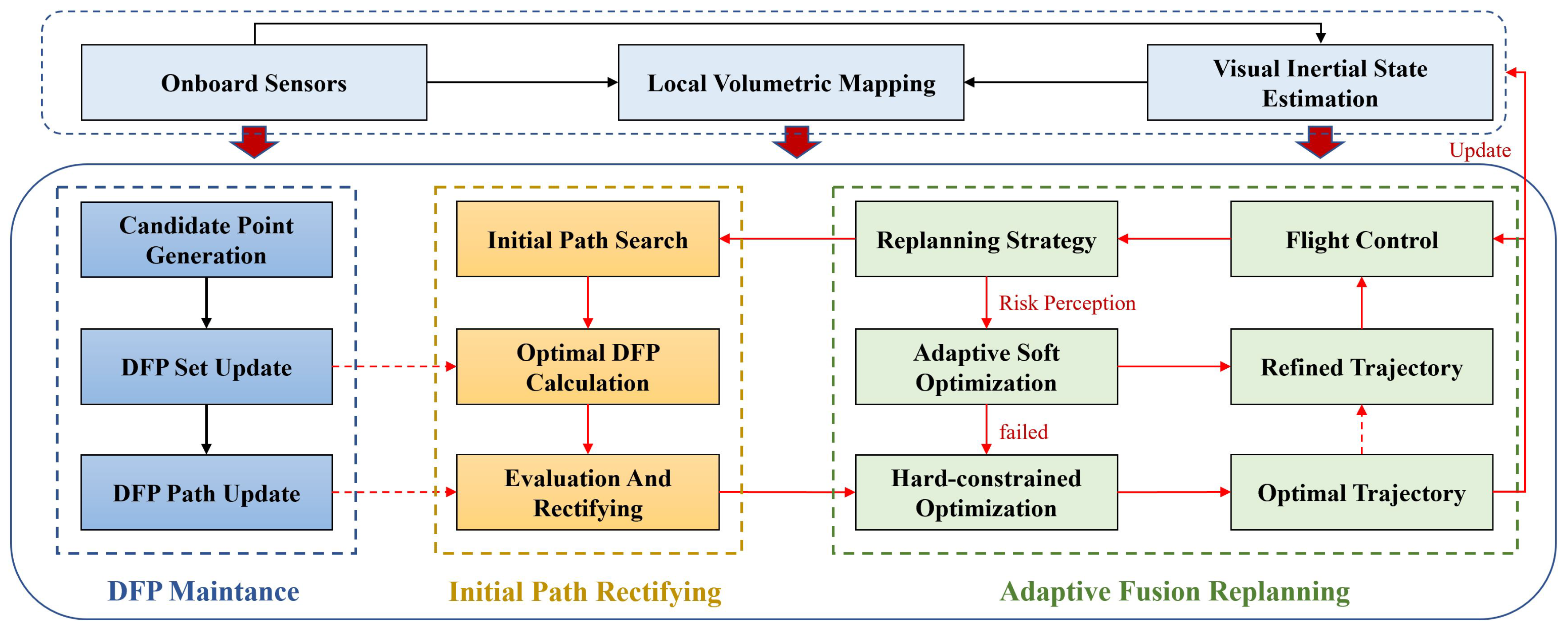
The framework of the proposed method is shown in Figure 1, composed of an incremental update of the DFP (Section 3.1 and Section 3.2), an initial path rectifying method (Section 3.3), and an adaptive fusion replanning method (Section 3.5). First, we design a directed frontier point information structure DFP to store the information of unexplored areas, which not only can provide an optimal DFP target and corresponding collision-free path for the local planner, but also can be continuously updated in real time with limited cost as the sensors move. Second, according to the guiding of DFP, the initial path generated by the local planner will be evaluated and rectified at the global level when necessary to avoid getting stuck in traps. Finally, an adaptive fusion replanning method is used to generate the local high-quality trajectory efficiently based on the corrected initial path.

3. Proposed Approach

3.1. Directed Frontier Point Information Structure

Generally, to avoid the local planner getting stuck in traps, high-frequency global path searching in a global map is used. This is obviously inefficient because a global map is needed, and the search process is time-consuming. To solve this, we design DFP and use it to both capture the frontier information of the explored space covered by the sensor and provide global guiding efficiently without maintaining the traditional global map. The data structure of DFP designed in this paper is shown in

Table 1. Data contained by a DFP $F{P}_i$ in the set $DFPs$.

Data	Explanation
$Po{s}_i$	Position of frontier point
$U{O}_i$	Orientation of unexplored space
$Pat{h}_i$	Collision-free path between the frontier point and the UAV

, which stores the position $Po{s}_i$ of the directed frontier point, the orientation $U{O}_i$ of the unknown space, and the collision-free geometric path $Pat{h}_i$ from the directed frontier point to the current position of the UAV. We use the set $DFPs$ of the directed frontier points to store the frontier points, which can be updated continuously by new data from sensors. Based on the set, we can rectify the local planner by selecting the optimal DFP (introduced in Section 3.3).

3.2. Directed Frontier Point Generation and Update

In order to obtain the DFP and provide the guiding efficiently, we design a generation-and-update method, as shown in Algorithm 1.

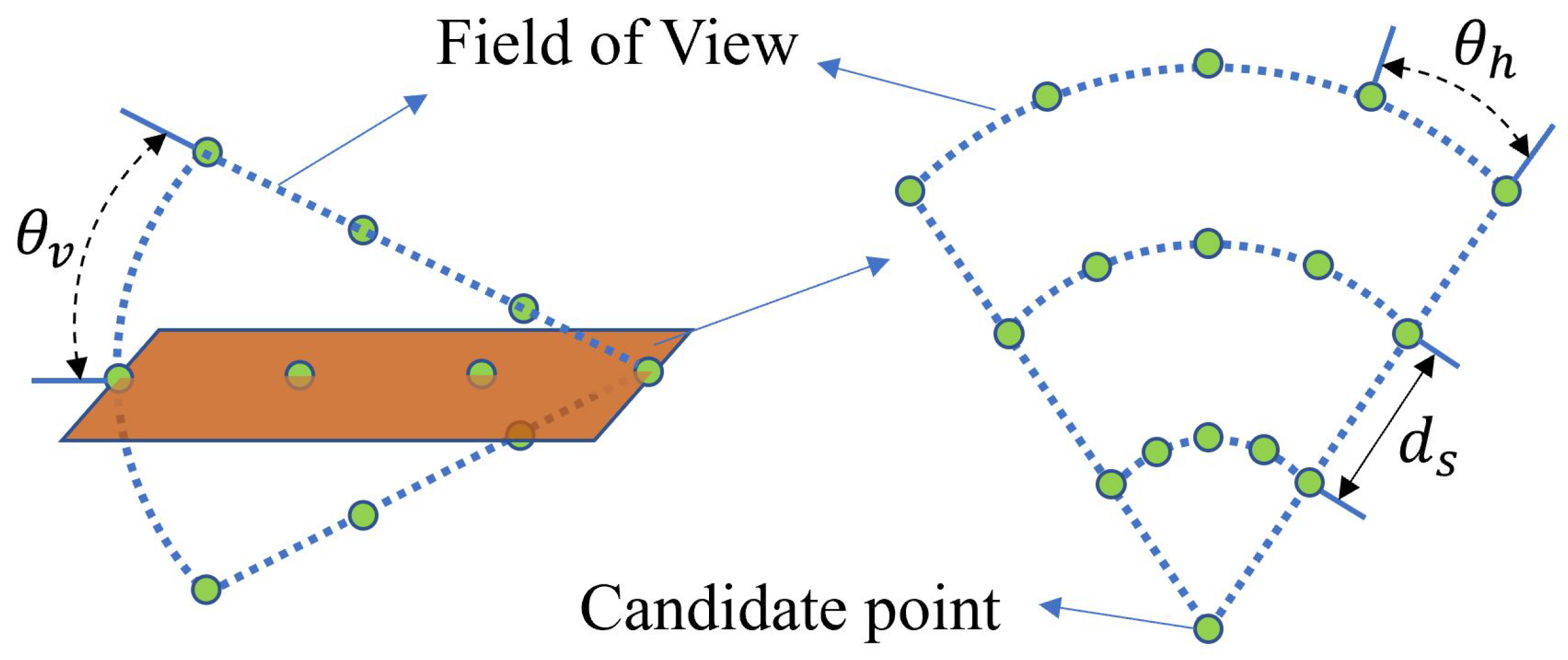
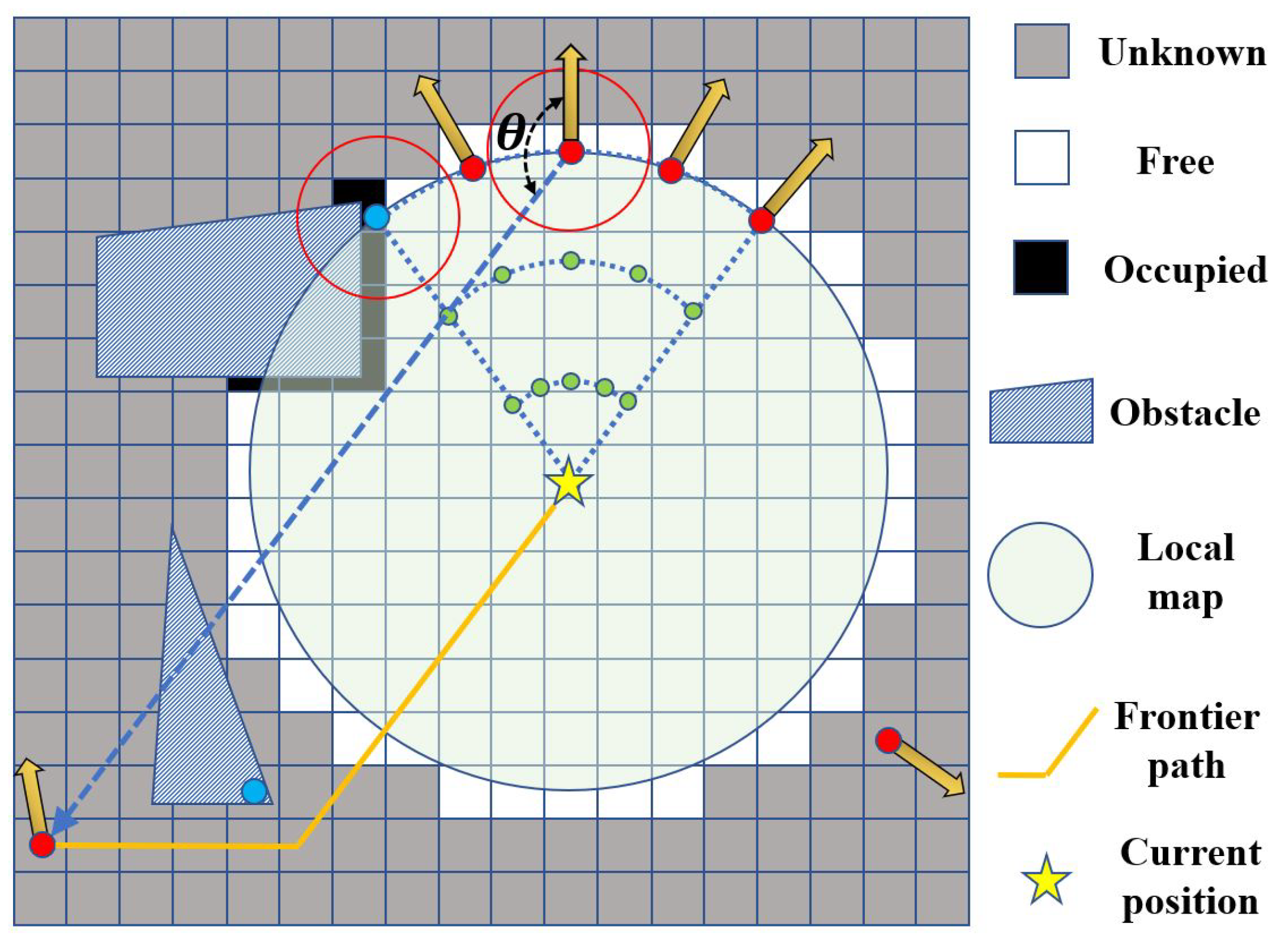
At first, as shown in Figure 2, the candidate directed frontier points $CPs$ are generated by using $\mathbf{SamplingInFOV}\mathbf{\left(}\mathbf{\right)}$ to sample points in the field of view (FOV) based on the state $X_0(p_0,{\xi }_0)$ of UAV and the information from sensors (Line 1). $p_0$ and ${\xi }_0$ represent the current position and yaw of the UAV, respectively. The max sampling range depends on the FOV and the maximum detection distance $r_s$ of the sensor, while the sampling interval’s distance and angle are determined by the minimum safe flight space that the UAV can pass. Then, as shown in Figure 3, each candidate point is judged in turn to select the points based on the following steps: (1) we use $\mathbf{CheckOccupiedPoint}\mathbf{\left(}\mathbf{\right)}$ to find the points in or near obstacles and add the points to the set of obstacle points $OPs$ (Line 3–5); (2) $\mathbf{CheckDFPConditions}\mathbf{\left(}\mathbf{\right)}$ is used to select the candidate points as the directed frontier points, and they are added to $DFPs$, which needs the points to meet conditions that contain both the unknown space and the free space in local (red circle) and that are inter-visible with the current position $p_0$ (Line 6); (3) once the candidate point meets the conditions of (2), we use $\mathbf{CalculateUnknownDir}\mathbf{\left(}\mathbf{\right)}$ to obtain the orientation $U{O}_i$ of unexplored space in $Po{s}_i$. Next, $\mathbf{CheckSamePoint}\mathbf{\left(}\mathbf{\right)}$ and $\mathbf{CheckPointInOPs}\mathbf{\left(}\mathbf{\right)}$ are used to check if similar points already exist in $DFPs$ and $OPs$. If the point is a unique point, we will add it to $DFPs$ (Line 7–15). Finally, in order to quickly provide a guiding path for the local planner without maintaining a global map when necessary, we use $\mathbf{UpdateDFPsPath}\mathbf{\left(}\mathbf{\right)}$ to update $Pat{h}_i$ for each $F{P}_i$ in real time, which is a collision-free path from the directed frontier point $F{P}_i$ to the current position $p_0$ of the UAV. In this way, inefficient global path searching is omitted. The detailed update process is described in Algorithm 2.

Algorithm 1 DFP generation and update.

Input: $X_0(p_0,{\xi }_0),DFPs,OPs$

Output: $DFPs,OPs$ 1: $CPs\leftarrow \mathbf{SamplingInFOV}\left(X_0\right)$ 2: for each $cp\in CPs$ 3:     if CheckOccupiedPoint($cp$) then 4:         $OPs$.add($cp$) 5:         $\mathbf{continue}$ 6:     if CheckDFPConditions($cp,X_0$) then 7: $UO\leftarrow \mathbf{CalculateUnknownDir}\left(cp\right)$ 8: $samePoint\leftarrow$ false 9:          for each $dfp\in DFPs$ 10:            if CheckSamePoint($cp,dfp$) then 11:                $samePoint\leftarrow$ true 12:         if $!samePoint$ then 13:             $samePoint\leftarrow \mathbf{CheckPointInOPs}\mathbf{(}\mathbf{cp}\mathbf{,}\mathbf{OPs}\mathbf{)}$ 14:         if $!samePoint$ then 15:             $DFPs.$add($cp$) 16: $\mathbf{UpdateDFPsPath}\mathbf{\left(}\mathbf{DFPs}\mathbf{\right)}$ 17: return $DFPs,OPs$

Since we only maintain a local map, we need to update the frontier path $Pat{h}_i$ for each $F{P}_i$ in real time to ensure that all parts of the path remain collision-free with limited cost. Firstly, we judge the $Pat{h}_i$ (represented by $path$ in Algorithm 2) of each node (Line 1–2). If the distance between the last node and the current position $p_0$ is greater than $r_s$, we add $p_0$ to the end of $Pat{h}_i$ (Line 3–5, 12–13). Otherwise, we use CheckVisibility() to judge the inter-visibility between $p_0$ and the node. Once it is inter-visible, the part of $Pat{h}_i$ after the node will be removed (Line 7–8). If the last node is not inter-visible with $p_0$, GetVertexPoint() will be used to calculate the vertex point and add it to the end of $Pat{h}_i$; therefore, the vertex point is inter-visible with the last node and $p_0$ at the same time (Line 9–11).

Algorithm 2 Frontier path update of DFP.

Input: $p_0,r_s,DFPs$

Output: $DFPs$ 1: for each $dfp\in DFPs$ 2:     $path\leftarrow dfp.Path$ 3:     $N\leftarrow path$.size() 4:     for $0\le j<N$ do 5:         $dist\leftarrow (path\left[j\right]-p_0)$.norm() 6:         if $dist$ < $r_s$ then 7:             if CheckVisibility $(path\left[j\right],p_0,vertex)$ then 8:                 $path$.erase($path$.begin()+j+1, $path$.end()) 9:             else if $j==N-1$ then 10:                $vertex\leftarrow \mathbf{GetVertexPoint}(path\left[j\right],p_0)$ 11:                $path$.add($vertex$) 12:        else if $j==N-1$ then 13:            $path$.add($p_0$) 14: return $DFPs$

3.3. Local Path Seaching and Rectifying

The initial path generation is critical, as its quality directly affects the efficiency of the path optimization and the success rate of the flight. Most of the existing methods adopt the kinodynamic path searching method (KPS) [17], A* [35], or jump point searching (JPS) [16] to find the initial path. KPS is a method that originated from the hybrid-state A* search, which can generate a safe and kinodynamically feasible trajectory, but it has low efficiency in some complex environments due to control space sampling. A* and JPS are well-known path searching methods that can quickly search a collision-free geometric path, but they do not consider the feasibility of dynamics. In order to search a high-quality initial path with a high success rate, we adopt a fusion searching strategy. We first use KPS to search the initial path $pat{h}_{initial}$ in local based on the motion state and dynamic constraints of the UAV. However, since KPS depends on the discrete control space during the search process, it will be difficult to find a high-quality path in a short time when the environment becomes complex. Therefore, to ensure the efficiency and stability of the initial path search, once KPS fails or the time cost exceeds the maximum time set by us, A* is performed.

However, since only the local map is maintained for planning, we can not blindly trust the search result, because it is easy to get into traps or continuous back-and-forth maneuvers if only the above method is used in unknown complex environments. To solve this problem, DFP is useful. At first, based on the motion state of the UAV and the target position, an optimal frontier point target $F{P}_{opt}$ is selected from $DFPs$ by solving the problem:

$$\begin{array}{c}\hfill \begin{array}{c}\hfill \underset{F{P}_i}{argmin}{\gamma }_1{f}_c+{\gamma }_2{f}_g+{\gamma }_3{f}_{dc}+{\gamma }_4{f}_{dg}={\gamma }_1{∥Po{s}_i-p_0∥}_2\\ \hfill +{\gamma }_2{∥p_g-Po{s}_i∥}_2+{\gamma }_3{∥\overrightarrow{U{O}_i}-\overrightarrow{v}∥}_2+{\gamma }_4{∥\overrightarrow{PG}-\overrightarrow{U{O}_i}∥}_2\end{array}\end{array}$$

(1)

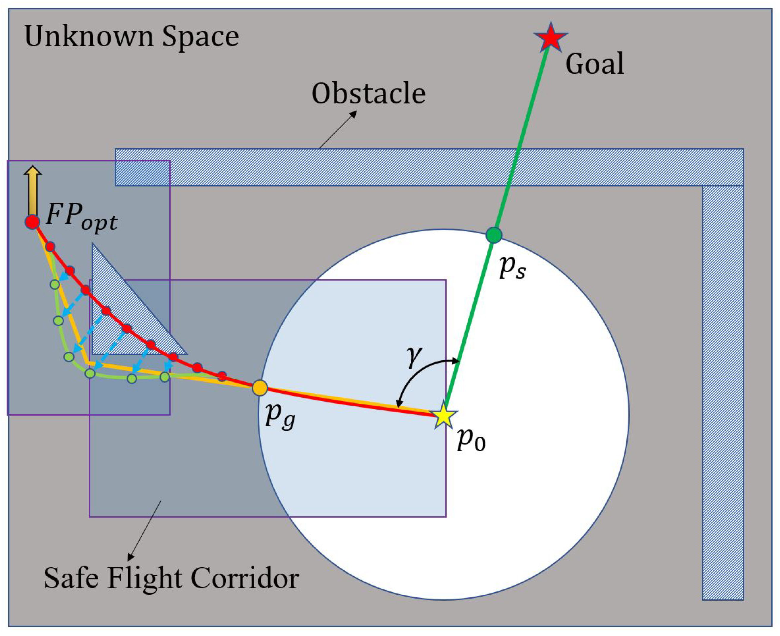
where $f_c$ represents the distance between the directed frontier point $F{P}_i$ and the current position $p_0$; $f_g$ represents the distance between $F{P}_i$ and the goal point $p_g$; $f_{dc}$ denotes the angle deviation between the orientation $\overrightarrow{U{O}_i}$ of unexplored space of $F{P}_i$ and the current motion direction $\overrightarrow{v}$; $f_{dg}$ denotes the angle deviation between $\overrightarrow{U{O}_i}$ and $\overrightarrow{PG}$, where $\overrightarrow{PG}$ is the orientation between $F{P}_i$ and $p_g$; and ${\gamma }_1$, ${\gamma }_2$, ${\gamma }_3$, and ${\gamma }_4$ are the coefficients of the above four items, respectively. We use this energy cost function to find the point with the lowest energy cost as the local optimal target point $F{P}_{opt}$ to the goal point. Then, as shown in Figure 4, we make a quality evaluation of the initial path $pat{h}_{initial}$ (green path, generated by KPS or A*) by comparing the path $pat{h}_{opt}$ of $F{P}_{opt}$ with $pat{h}_{initial}$. If the deviation angle $\gamma$ is less than ${\gamma }_0$ (typically ${\gamma }_0\approx {45}^{\circ }$), we consider the path $pat{h}_{initial}$ to be plausible. The path is then normally used for path optimization. Otherwise, we consider $pat{h}_{initial}$ to not be credible, and we will rectify the flight direction by directly using the collision-free path $pat{h}_{opt}$ maintained by $F{P}_{opt}$ as the initial path for path optimization.

3.4. Adaptive Fusion Replanning

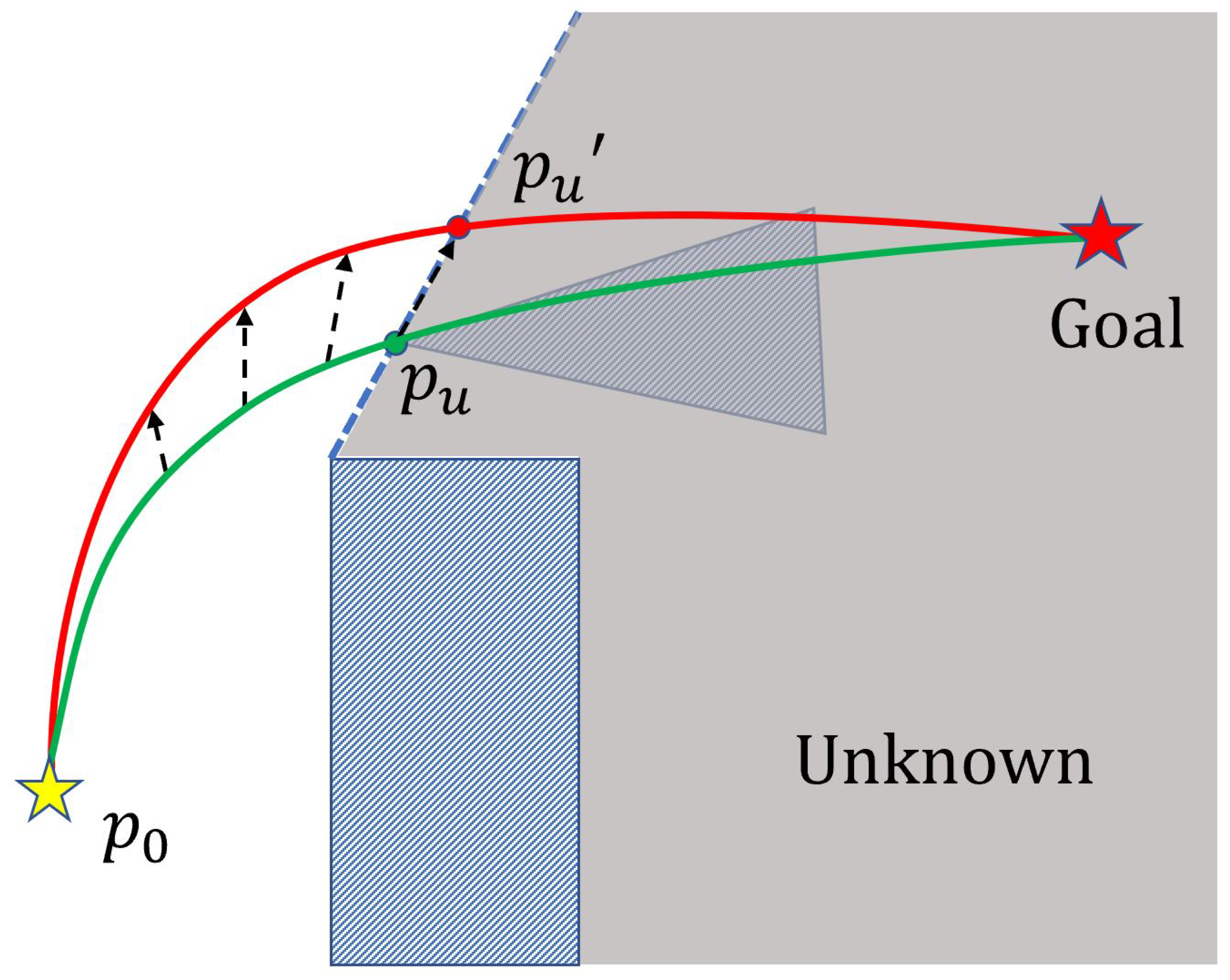
Although the initial path can be generated by Section 3.3, the path is not optimal in theory due to the discrete control space and the lack of consideration for trajectory smoothness. Therefore, after determining the initial path, we will optimize the trajectory in terms of smoothness, safety, and dynamic feasibility to improve the trajectory quality. Currently, trajectory optimization mainly uses the hard-constrained method or the soft-constrained method. The quality of the path generated by the former is high, but its planning efficiency is relatively low. The planning efficiency of the latter is high, but the trajectory generated by the method may not strictly satisfy the pre-set constraints. Different from the existing methods, as shown in Figure 4, we design an adaptive fusion replanning strategy by elaborating the advantages of both optimization methods, which will use different methods depending on the situation: the former for quality and the latter for safety.

First, we generate the optimal flight trajectory based on the initial path by solving the problem:

$$\begin{array}{cc}\hfill \underset{\mathrm{p}\left(t\right),T}{min}& {\int }_0^{T}u{\left(t\right)}^{\mathrm{T}}\mathbf{W}u\left(t\right)\mathrm{d}t+\rho \left(T\right),\hfill \\ \hfill \mathrm{s}.\mathrm{t}.& u\left(t\right)={\mathrm{p}}^{\left(s\right)}\left(t\right),\forall t\in [0,T],\hfill \\ \hfill & \mathcal{G}\left(\mathrm{p}\left(t\right),\dots ,{\mathrm{p}}^{\left(s\right)}\left(t\right)\right)⪯0,\forall t\in [0,T],\hfill \\ \hfill & \mathrm{p}\left(t\right)\in \mathcal{F},\forall t\in [0,T],\hfill \\ \hfill & {\mathrm{p}}^{[s-1]}\left(0\right)={\overline{\mathrm{p}}}_o,{\mathrm{p}}^{[s-1]}\left(T\right)={\overline{\mathrm{p}}}_f,\hfill \end{array}$$

(2)

where $\mathrm{p}\left(t\right)$ represents the trajectory; T and $\mathbf{W}$ are the trajectory time and a positive diagonal matrix; $u\left(t\right)$ represents the control input; ${\overline{\mathrm{p}}}_o$ and ${\overline{\mathrm{p}}}_f$ denote the initial condition and the terminal condition; $\rho \left(T\right)$ represents the time regularization to trade off between the control effort and the expectation of total time; $\mathcal{G}\left(\mathrm{p}\left(t\right),\dots ,{\mathrm{p}}^{\left(s\right)}\left(t\right)\right)$ is used to meet the user-defined state-input constraints. To ensure safety of the trajectory, we constrain the trajectory $\mathrm{p}\left(t\right)$ in $\mathcal{F}$ that is the obstacle-free area in the configuration space (purple area in Figure 4). To solve the problem efficiently, we use the same method as in [26], which bridges the gaps among solution quality, planning efficiency, and constraint fidelity with limited resources and maneuvering capability compared with other methods. Its generality and robustness have also been verified by extensive experiments and applications. We refer the readers to [26] for more details about the problem solving method. Due to the high quality of the path generated by the above method, we regard the path as the optimal path (red path) to execute.

Due to the limited sensing range, we plan in both the known space and in the unknown space to improve the flight speed and reduce the planning cost; however the safety of the whole flight trajectory can not be guaranteed. At the same time, the path generated by the above optimization method makes it easy to get close to obstacles, and the planning process often takes a long time. Therefore, to ensure safety and achieve real-time and efficient obstacle avoidance, once there are new obstacles that affect the safety of the flight trajectory, the soft-constrained method is adopted to optimize the trajectory in local based on its high efficiency in planning. In this part, uniform B-spline is used to represent the trajectory. Due to the convex hull characteristics of the B-spline, it is easy to optimize the trajectory to meet the requirements of safety and smoothness by changing the position of its control points. Therefore, we can optimize its safety, smoothness, and dynamic feasibility by solving the problem:

$$\begin{array}{c}\hfill \begin{array}{c}\hfill \underset{Q}{min}J={\lambda }_1{J}_s+{\lambda }_2{J}_c+{\lambda }_3{J}_d,\end{array}\end{array}$$

(3)

where Q is the control point of the B-spline; $J_s$, $J_c$, and $J_d$ represent the penalty items of smoothness, collision, and feasibility, respectively; and ${\lambda }_1$, ${\lambda }_2$, and ${\lambda }_3$ are penalty weights for each items. To free the optimization method from ESDF and make the planning efficient, we follow the work of [18] in calculating the penalty items, especially the $J_c$:

$$F_c\left(Q_i\right)=\left\{\begin{array}{cc}0& (c_i\le 0)\\ c_i^3& (0<c_i\le s_f),\\ 3s_f{c}_i^2-3s_f^2{c}_i+s_f^3& (c_i>s_f)\end{array}\right.$$

(4)

$$c_i=s_f-d_i$$

(5)

$$j_c=\sum _{i=1}^{N_c}{F}_c\left(Q_i\right),$$

(6)

where $F_c\left(i\right)$ is the collision cost for control point $Q_i$; $d_i$ is the obstacle distance from $Q_i$ to the obstacle, which is calculated by an anchor point at the obstacle surface with a corresponding repulsive direction vector generated by a collision-free path $p_f$ and which frees the planner from ESDF; and $s_f$ represents the safety clearance. Therefore, due to the special design, it is easy to obtain the gradient by directly computing the derivative of $F_c$ with respect to $Q_i$. More details about the penalty items can be found in [18].

In addition, different from the other methods that use the optimization function with fixed penalty weights for all complex and changeable environments, we adopt an adaptive optimization method as in our previous work [33], which can improve the planning quality and planning success rate by using different parameters to optimize the trajectory according to the changing environment. To achieve this, when $p_f$ (mentioned above, yellow path in Figure 4) is obtained to optimize the trajectory away from obstacles (details can be found in [18]), we perceive the environment and obtain the distance $d_s$ of the narrowest passage based on the path. Once the environment is narrow, we make safety an optimization priority by improving the weight of the collision penalty. Meanwhile, inspired by [16,32], we add another adjustment strategy to improve the safety of the flight around the corners. As shown in Figure 5, we use the normal optimization when the distance $d_{ou}$ between the intersection point $p_u$ and the current position $p_0$ satisfies the minimum safety condition:

$$\begin{array}{c}\hfill \begin{array}{c}\hfill v_c^2/2a_{max}\le d_{ou}-R_q.\end{array}\end{array}$$

(7)

If the condition is not satisfied, we can improve the safety of the path by lengthening the distance $d_{ou}$, which can be satisfied by pushing the trajectory far from obstacles. According to the above theory, ${\lambda }_1$ and ${\lambda }_2$ can be formulated as follows:

$${\lambda }_1=F_{{\lambda }_1}\left(d_s\right)=\left\{\begin{array}{ccc}\hfill & {\lambda }_1^{\prime }\hfill & \hfill d_s>d_n\\ \hfill & {\lambda }_1^{\prime }-{\gamma }_1(1-\frac{d_s}{d_n})\hfill & \hfill d_s\le d_n\end{array}\right.$$

(8)

$${\lambda }_2=F_{{\lambda }_2}(d_s,d_u)=\left\{\begin{array}{ccc}\hfill & {\lambda }_2^{\prime }\hfill & \hfill d_s>d_n\\ \hfill & {\lambda }_2^{\prime }+{\gamma }_2(1-\frac{d_s}{d_n})\hfill & \hfill d_s\le d_n\\ \hfill & {\lambda }_2^{\prime }+{\gamma }_2{d}_u\hfill & \hfill d_u\ge 0\end{array}\right.$$

(9)

$$\begin{array}{c}\hfill \begin{array}{c}\hfill d_u=v_c^2/2a_{max}+R_q-d_{ou},\end{array}\end{array}$$

(10)

where ${\lambda }_1^{\prime }$ and ${\lambda }_2^{\prime }$ represent the initial smoothness weight and the initial collision weight, respectively; ${\gamma }_1$ and ${\gamma }_2$ are the weights for adjusting ${\lambda }_1$ and ${\lambda }_2$; $d_n$ is a threshold that can be used to find a narrow space; and $d_u$ indicates the difference to meet Equation (7).

3.5. Replanning Strategy

Due to the limited sensing and planning range, we have to replan the trajectory frequently to ensure the quality of the flight trajectory when the UAV flies in an unknown environment. To make the above process stable and efficient, a replanning strategy is designed: (1) when the flight time exceeds half the duration of the trajectory generated by the hard-constrained method, the method is triggered again to regenerate the flight trajectory; (2) when the newly discovered obstacles affect the safety of the current trajectory, the soft-constrained method is triggered to quickly optimize the trajectory in local; (3) once the replanning by the soft-constrained method fails or the path provided by DFP is adopted, the hard-constrained method is used to generate the trajectory again; and (4) when the target point appears in the field of view, the hard-constrained method is triggered to generate the final trajectory and stop the replanning part. In this way, we consider both the quality of the trajectory and the rapid response to the newly discovered obstacles.

4. Experimental Results

4.1. Benchmark Comparisons

In the simulation experiment, we compare the proposed method with several state-of-the-art methods in different environments: FASTER [16], EGO-Planner [18], and Fast-Planner [17]. FASTER is a typical method that belongs to the hard-constrained category. EGO-Planner and Fast-Planner are two well-known soft-constrained methods for real-time UAV motion planning and have achieved good results. We adopt its open-source implementation and default configuration. Meanwhile, it should be noted that the dynamic limits we used in all simulation experiments are $v_{max}=3.0$ m/s and $a_{max}=2.0$ m/${\mathrm{s}}^2$ for each method. The FOVs of the sensors are set as [$80\times 60$] deg with a maximum range of 4.5 m. Additionally, all experiments are conducted on a computer with an Intel Core i9-9900K@ 3.6 GHz, 64 GB memory, and ROS Melodic.

4.1.1. Random Scenario

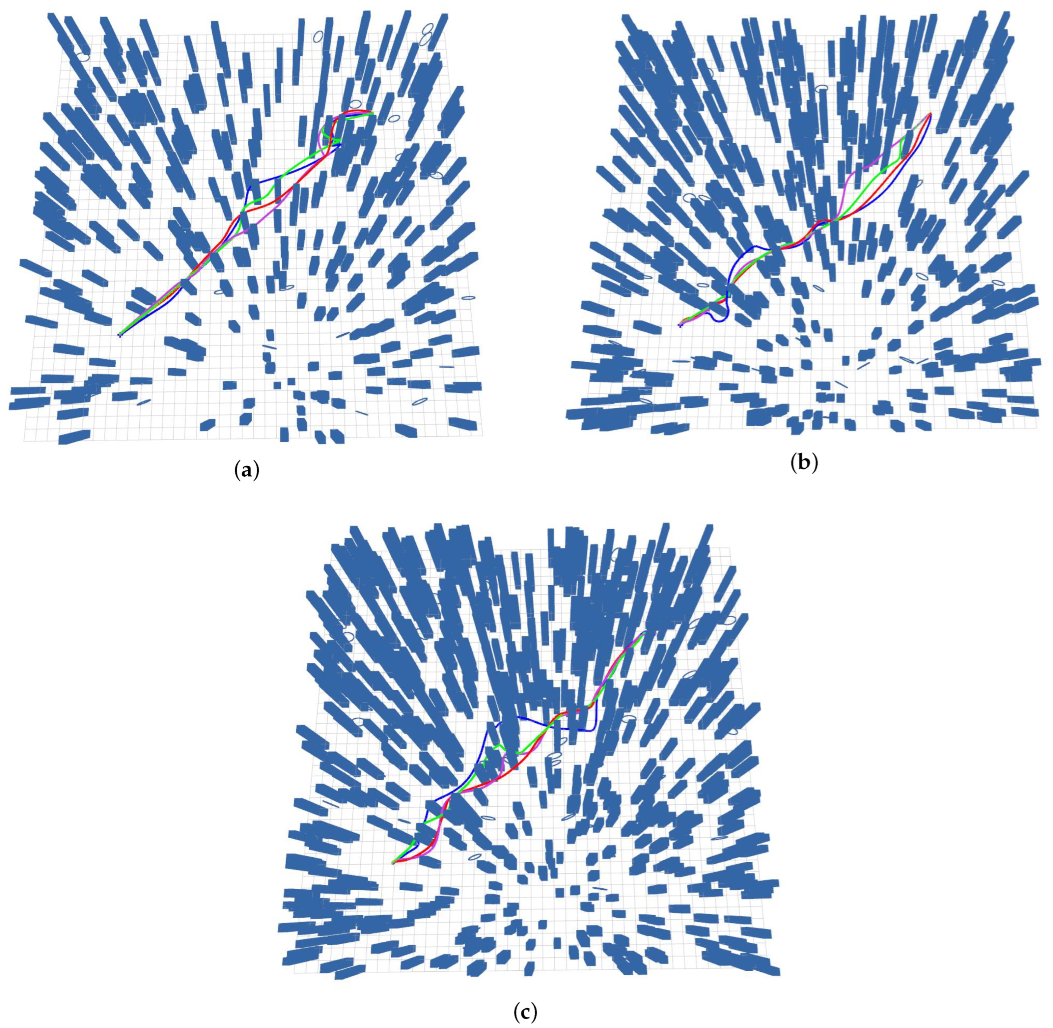
At first, we conducted a comparison experiment of the four methods in 40 × 40 × 3 m random environments containing three different obstacle densities: 0.2 obstacles/${\mathrm{m}}^2$, 0.3 obstacles/${\mathrm{m}}^2$, and 0.4 obstacles/${\mathrm{m}}^2$. Three maps were randomly generated for each obstacle density, and each method was tested 10 times in a map under the same experimental conditions. Samples of the maps and the flight trajectories are shown in Figure 6. The detailed result of the experiments is shown in

Table 2. Flight statistics in random scenarios with different obstacle density.

Scene	Method	Flight Time (s)			Flight Distance (m)			Energy (${\mathrm{m}}_2/{\mathrm{s}}^5$)			Replan Time (ms)	Success Rate (%)
		Avg	Std	Max	Avg	Std	Max	Avg	Std	Max
0.2 obs/m${}^2$	Fast-Planner	15.95	1.5	18.47	35.67	1.06	37.44	255.02	87.2	400.91	3.2	86
	FASTER	15.38	2.5	21.66	33.85	2.4	39.23	125.47	32.2	174.98	29.9	93.3
	EGO-Planner	15.14	1.7	19.67	33.35	1.0	35.15	215.02	44.7	286.98	1.9	100
	Proposed	15.69	0.3	16.34	33.48	0.6	34.32	168.22	62.2	261.10	3.3	100
0.3 obs/m${}^2$	Fast-Planner	18.27	2.1	20.66	36.65	1.5	38.70	339.36	101.9	510.59	3.2	80
	FASTER	17.66	2.2	21.36	33.73	1.0	35.91	196.02	58.2	339.10	34.9	86
	EGO-Planner	17.20	2.4	21.93	35.37	1.7	37.79	431.66	112.7	675.38	2.5	93
	Proposed	17.45	2.1	23.31	34.66	1.4	37.20	267.08	75.3	472.30	3.9	100
0.4 obs/m${}^2$	Fast-Planner	24.76	4.4	31.61	37.63	2.2	40.84	675.38	168.85	952.41	3.4	33.3
	FASTER	23.78	2.7	27.71	36.07	2.3	41.71	329.47	71.0	464.19	41.0	53.3
	EGO-Planner	17.80	1.8	22.52	35.87	1.1	38.83	464.22	126.8	762.39	2.4	66.7
	Proposed	18.64	1.8	21.60	35.75	1.2	38.17	304.06	66.5	462.58	4.8	100

.

It can be seen that Fast-Planner performs relatively poorly, and its planning success rate decreases significantly with the increase in obstacle density. This is because the method incorporates the gradients of ESDF in a collision cost to push the trajectory out of the way of the obstacles, and the cost is combined with the smoothness and dynamic feasibility cost to form an objective function. Therefore, the method will always encounter local minima problems resulting in optimization failure when there are valleys or ridges in scenarios. In addition, the method generates the initial kinodynamic path using discrete control space, which will cause detours due to the loss of solution space when the obstacle density becomes high. Since EGO-Planner proposes a lightweight yet effective trajectory refinement algorithm, it achieves the highest planning efficiency and the best performance in terms of flight time and flight distance. Meanwhile, due to the help of the guiding path, the method avoids the local minima problems, and its planning success rate performs better compared to Fast-Planner. However, the method is overly dependent on its reference path (the line between the start point and end point), which will cause unnecessary detours and influence the flight performance in some scenarios. FASTER is a hard-constrained method that can generate a high-quality trajectory, so its trajectory energy cost is the best. However, it takes much more time than other methods because it needs to solve two trajectories for safety in the constructed SFC at the same time. Since the method takes the result of jump point search (JPS) as the initial path that does not consider dynamic feasibility, the success rate of and quality of the optimization will be affected. It can be seen that our method achieves a more balanced result compared to the above three methods. This is because we realize the advantages of different optimization methods while reducing the influence of their drawbacks by designing an adaptive fusion replanning method, which fuses the hard-constrained with soft-constrained methods by using a reasonable replanning strategy to compensate for the shortcomings of one another. Specifically, we preferentially execute the trajectory generated by the hard-constrained method, and the soft-constrained method is adopted to optimize the flight trajectory to avoid new obstacles in local. Therefore, our method takes advantage of both the high quality of the trajectory generated by the hard-constrained method and the high efficiency of the soft-constrained method (EGO-Planner). The experimental results also verify our theory. The planning efficiency of our method is much higher than FASTER and is similar to EGO-Planner and Fast-Planner. The energy cost of our method is only slightly higher than FASTER. Meanwhile, compared with EGO-Planner, since we use the hard-constrained method to keep updating our reference trajectory instead of using the straight line between the start point and the end point all the time, our flight trajectory is more smooth and reasonable than EGO-Planner. In addition, since we use a guiding path to help the optimization and can adjust the focus of the optimization according to the actual environment, our method can avoid the local mimima problem and pass through narrow areas easily. These help our method achieve the best performance of the four methods in terms of success rate, and these experimental results also cover our contribution to adaptive fusion replanning.

4.1.2. Office Scenario

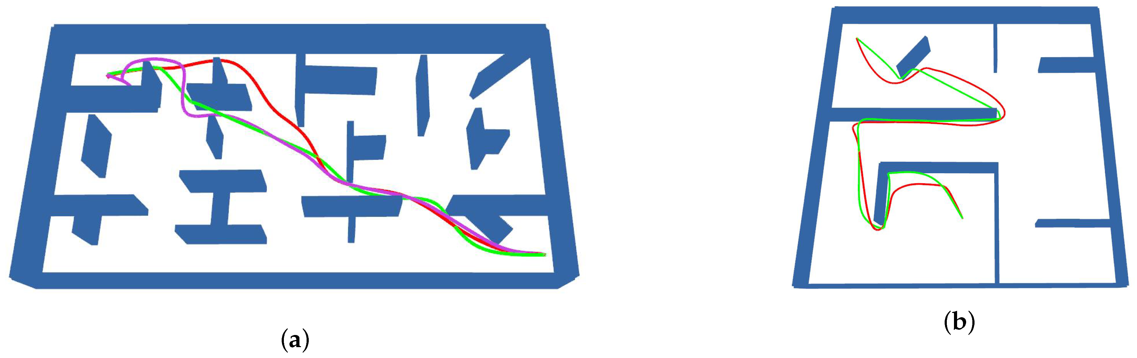
To verify the planning effectiveness and stability of each method in complex office scenarios that contain large obstacles, as shown in Figure 7, we compare the four methods in the two complex office scenarios (office-1 and office-2). Compared to random scenes that contain only small obstacles, the office scenarios are more complex, having not only small obstacles but also large obstacles and traps between the start point and the goal point. Therefore, these scenarios are closer to the real scenarios. The detailed experimental result is shown in

Table 3. Flight statistics in office scenarios containing large obstacles.

Scene	Method	Flight Time (s)			Flight Distance (m)			Energy (${\mathrm{m}}_2/{\mathrm{s}}^5$)			Replan Time (ms)	Success Rate (%)
		Avg	Std	Max	Avg	Std	Max	Avg	Std	Max
Office-1	Fast-Planner	/	/	/	/	/	/	/	/	/	/	0
	FASTER	17.39	2.9	25.64	32.43	4.8	46.39	178.89	40.8	255.24	39.7	100
	EGO-Planner	19.55	1.8	22.44	33.32	1.0	34.33	303.03	35.3	331.54	3.3	80.0
	Proposed	17.72	2.4	22.93	33.06	2.9	38.10	176.65	49.0	296.79	4.8	100
Office-2	Fast-Planner	/	/	/	/	/	/	/	/	/	/	0
	FASTER	33.71	/	33.71	65.91	/	65.91	170.73	/	170.73	38.4	10.0
	EGO-Planner	/	/	/	/	/	/	/	/	/	/	0
	Proposed	32.93	1.7	35.41	67.51	2.0	71.29	198.90	43.0	272.37	9.8	100

. It can be seen from the results that, due to the limitation of the planning range and the lack of global information, EGO-Planner and Fast-Planner are not suitable for these environments, as the planning success rate for both methods is severely impacted, especially in office-2. Since FASTER maintains a larger local map, it performs better than the first two methods. However, its success rate is also low in office-2 because the scenario contains large obstacles between the start point and the goal point. Compared with the above three methods, our method can still operate stably in these scenes containing large obstacles. This is because of the directed frontier point information structure DFP that is designed in this paper, which can both roughly capture the frontier information of the explored environment and efficiently provide global-level guidance. Based on the global evaluation and rectifying of DFP, our method can work stably and will not get stuck in traps of large obstacles. In addition, to verify the efficiency of DFP, as shown in

Table 4. Average cost to maintain part of the DFP in different scenarios.

Scene	DFPs Update Time (ms)				DFPs Num.	OPs Num.
	Avg	Std	Max	Min
0.2 obs./m${}^2$	0.34	0.07	0.52	0.29	116.0	67.3
0.3 obs./m${}^2$	0.28	0.02	0.34	0.25	81.4	95.8
0.4 obs./m${}^2$	0.26	0.02	0.29	0.23	78.7	108.4
Office-1	0.17	0.03	0.28	0.17	45.1	73.0
Office-2	0.26	0.09	0.36	0.25	98.4	59.8

, we also provide the average cost of maintaining part of DFP in different scenarios. It can be seen that, although we added a new component to provide global rectifying compared with other methods, the computational burden added by this component is very limited, and there is no additional significant computational cost beyond a few hundreds points in each experiment. However, if more precise guidance is needed to reduce the probability of misdirection, the number of DFPs and the cost will increase gradually.

4.1.3. Further Evaluation

In addition, in order to compare the performance and stability of the four methods in different scenarios more visually, as shown in Figure 8, we provide the actual distribution of all experimental results (flight time, flight distance, and energy cost) for the four methods in different scenarios. It can be seen that the results of the distribution of the experimental data are the same as the previous analysis. In general, the indicators (flight time, flight distance, and energy cost) of the four methods all increase with the complexity of the scenario, and the fluctuation range of flight time also becomes larger. Although the experimental results of our method are not optimal in a certain indicator, our method is more balanced in all indicators and achieves better adaptability in all scenarios. However, due to the effect of directional rectifying, there is a fluctuation in flight efficiency because the DFP is obtained by sampling and its global guiding does not always make the best choice every time since the scenario is unknown.

4.2. Real-World Experiments

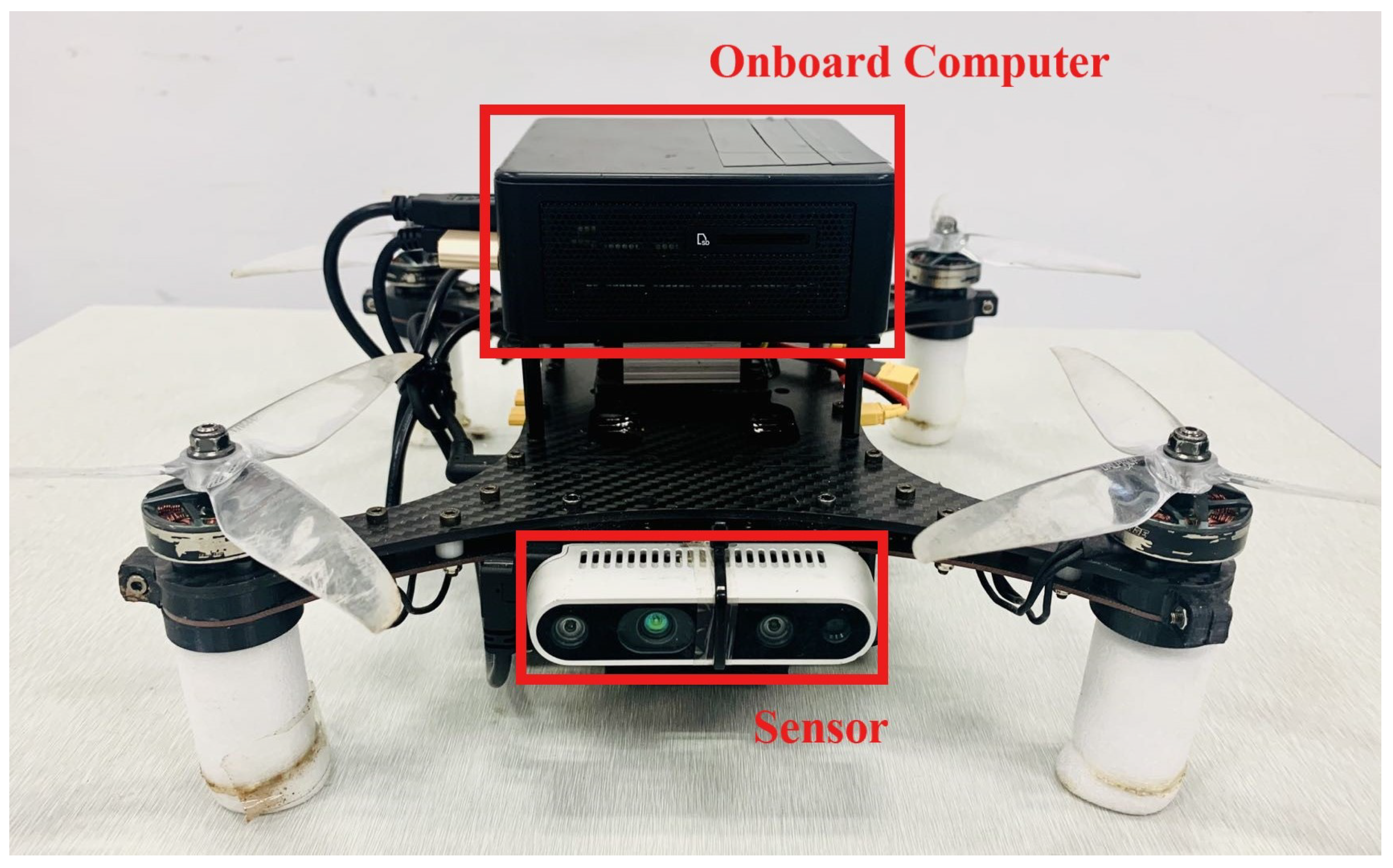
To verify the effectiveness of the proposed method, we also present real-world experiments in outdoor cluttered environments by using a customized quadrotor equipped with a forward-facing RealSense D435. The quadrotor is shown in Figure 9. In the experiments, we use [36] to provide the quadrotor state. All the modules run on an Intel Core i5-1135G7@ 2.40 GHz, 16 GB memory, and ROS Melodic.

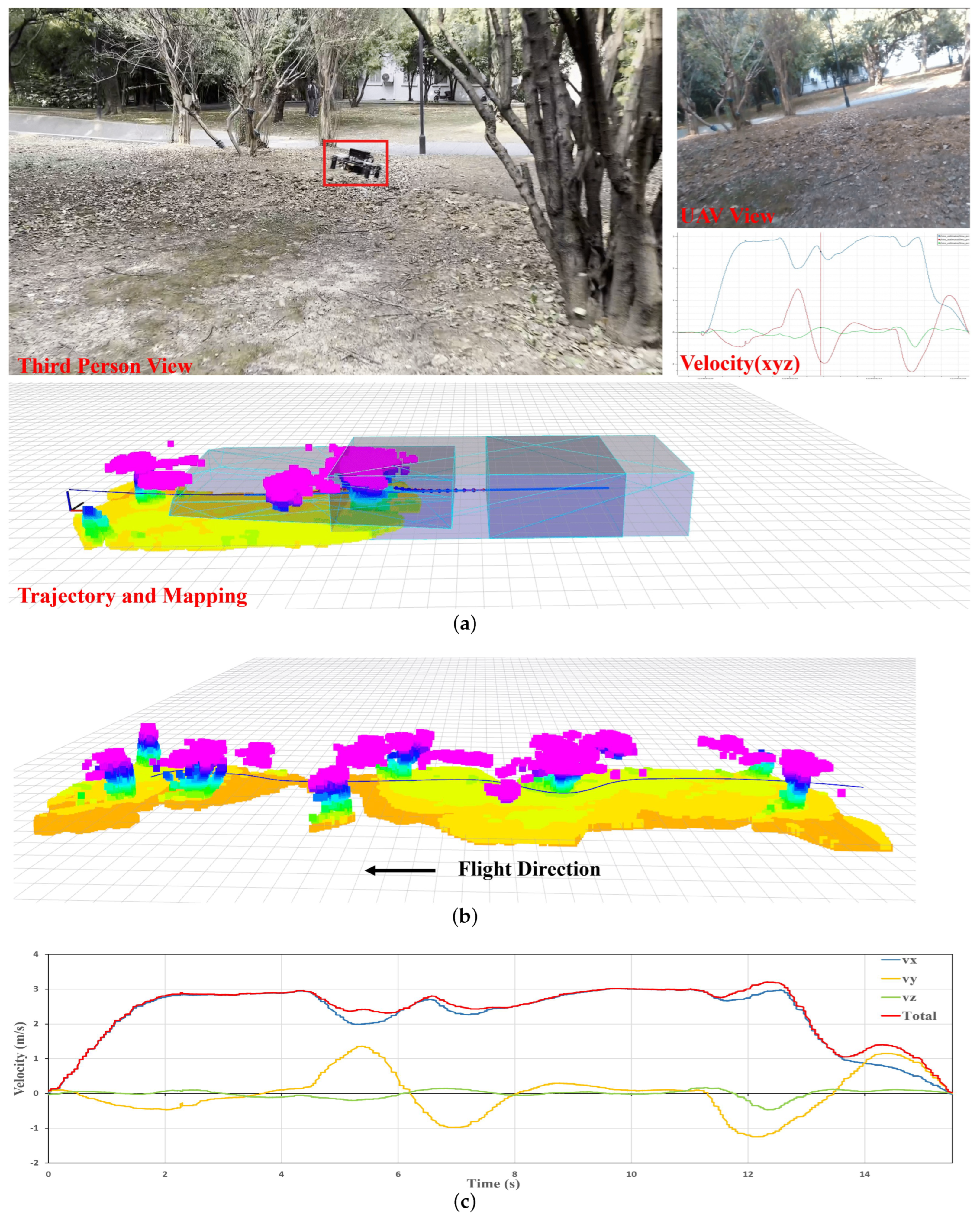
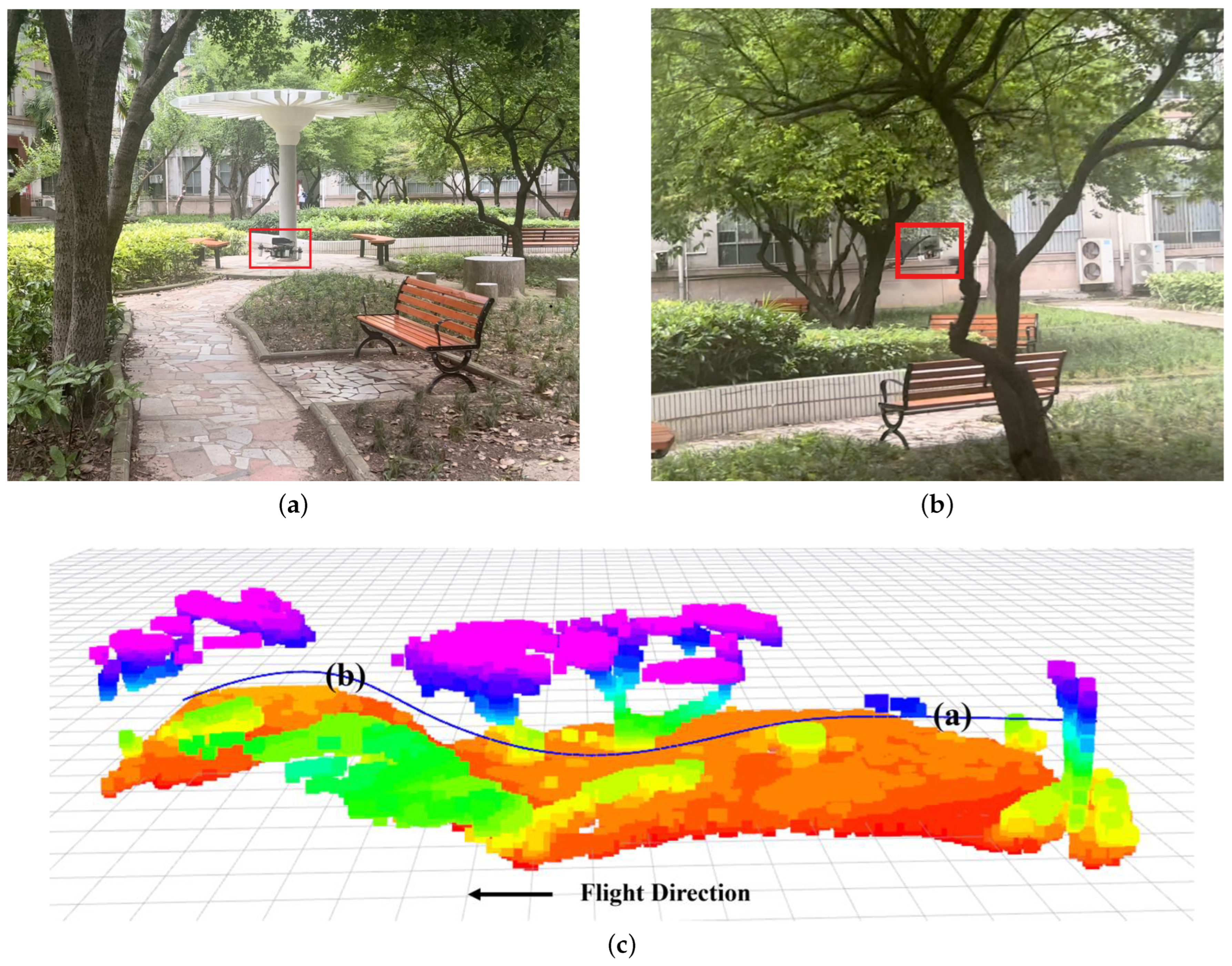
At first, as shown in Figure 10, we present experiments in a forested environment, which contains large trees and wire poles. The environment is typically unstructured and irregular, in which the quadrotor needs to perform agile maneuvers to avoid obstacles such as tree branches and leaves. In the experiment, the quadrotor flies through the forest to the goal 35 m away from the initial position. The velocity profile is shown in Figure 10c. The maximum speed and the average speed reach 3.21 m/s and 2.39 m/s, respectively. The flight takes 37.15 m and 15.51 s. The actual flight trajectory and the online generated map are shown in Figure 10b. From the experimental results, it can be seen that the actual flight trajectory of the UAV is smooth and the speed changes smoothly. In addition, we also conducted experiments in a park environment containing various types of obstacles. The experimental result is shown in Figure 11. The performances in the above two real-world experiments all prove the practicality and effectiveness of our method.

5. Conclusions

In this paper, we propose a robust planning framework for fast autonomous flight in a complex, unknown environment by using sparse directed frontier points. First, an incrementally sparse directed frontier point (DFP) is designed, which can both roughly record the position and direction of unreachable areas to provide global information with limited cost and efficiently maintain a collision-free geometric path from the UAV to the position. Second, supported by the DFP, the local initial path generated by the planner is evaluated, and the initial path is rectified at the global level when necessary. Then, an adaptive fusion replanning method is proposed to generate a high-quality trajectory efficiently, which incorporates two optimization methods with different characteristics to achieve quality and efficiency by a reasonable replanning strategy. In addition, an adaptive optimization function is also introduced to improve planning stability, which can adjust the focus of the optimization according to the actual environment. Sufficient benchmark experiments in simulation are conducted to verify the performance of our method. The result shows that, compared with other methods, we improve the planning quality while ensuring the higher planning efficiency by using the fusion replanning strategy. Meanwhile, since DFP can efficiently provide global-level guidance for the local planner, the planning success rate and the adaptability to the environment of our method are significantly improved compared to other methods. Moreover, the proposed system is integrated into a fully autonomous quadrotor, and the effectiveness of the proposed method is further evaluated by using the quadrotor in real-world environments.

References

- Wei, Z.; Zhu, M.; Zhang, N.; Wang, L.; Zou, Y.; Meng, Z.; Wu, H.; Feng, Z. UAV Assisted Data Collection for Internet of Things: A Survey. IEEE Internet Things J. 2022, 9, 15460–15483. [Google Scholar] [CrossRef]
- Wang, X.; Gursoy, M.C.; Erpek, T.; Sagduyu, Y.E. Learning-Based UAV Path Planning for Data Collection with Integrated Collision Avoidance. IEEE Internet Things J. 2022, 9, 16663–16676. [Google Scholar] [CrossRef]
- Zheng, X.; Wang, F.; Li, Z. A multi-UAV cooperative route planning methodology for 3D fine-resolution building model reconstruction. Isprs J. Photogramm. Remote. Sens. 2018, 146, 483–494. [Google Scholar] [CrossRef]
- Zhang, X.; Chu, Y.; Liu, Y.; Zhang, X.; Zhuang, Y. A novel informative autonomous exploration strategy with uniform sampling for quadrotors. IEEE Trans. Ind. Electron. 2021, 69, 13131–13140. [Google Scholar] [CrossRef]
- Wang, H.; Zhang, S.; Zhang, X.; Zhang, X.; Liu, J. Near-optimal 3-D visual coverage for quadrotor unmanned aerial vehicles under photogrammetric constraints. IEEE Trans. Ind. Electron. 2021, 69, 1694–1704. [Google Scholar] [CrossRef]
- Wu, Y.; Wu, S.; Hu, X. Cooperative path planning of UAVs & UGVs for a persistent surveillance task in urban environments. IEEE Internet Things J. 2020, 8, 4906–4919. [Google Scholar]
- Chen, S.W.; Nardari, G.V.; Lee, E.S.; Qu, C.; Liu, X.; Romero, R.A.F.; Kumar, V. Sloam: Semantic lidar odometry and mapping for forest inventory. IEEE Robot. Autom. Lett. 2020, 5, 612–619. [Google Scholar] [CrossRef] [Green Version]
- Qadir, Z.; Zafar, M.H.; Moosavi, S.K.R.; Le, K.N.; Mahmud, M.P. Autonomous UAV Path-Planning Optimization Using Metaheuristic Approach for Predisaster Assessment. IEEE Internet Things J. 2021, 9, 12505–12514. [Google Scholar] [CrossRef]
- Huang, Z.; Chen, C.; Pan, M. Multiobjective UAV path planning for emergency information collection and transmission. IEEE Internet Things J. 2020, 7, 6993–7009. [Google Scholar] [CrossRef]
- Yin, C.; Xiao, Z.; Cao, X.; Xi, X.; Yang, P.; Wu, D. Offline and online search: UAV multiobjective path planning under dynamic urban environment. IEEE Internet Things J. 2017, 5, 546–558. [Google Scholar] [CrossRef]
- Li, J.; Xiong, Y.; She, J.; Wu, M. A path planning method for sweep coverage with multiple UAVs. IEEE Internet Things J. 2020, 7, 8967–8978. [Google Scholar] [CrossRef]
- Liu, D.; Bao, W.; Zhu, X.; Fei, B.; Men, T.; Xiao, Z. Cooperative Path Optimization for Multiple UAVs Surveillance in Uncertain Environment. IEEE Internet Things J. 2021, 9, 10676–10692. [Google Scholar] [CrossRef]
- Yu, Z.; Si, Z.; Li, X.; Wang, D.; Song, H. A Novel Hybrid Particle Swarm Optimization Algorithm for Path Planning of UAVs. IEEE Internet Things J. 2022, 9, 22547–22558. [Google Scholar] [CrossRef]
- Shen, K.; Shivgan, R.; Medina, J.; Dong, Z.; Rojas-Cessa, R. Multi-Depot Drone Path Planning with Collision Avoidance. IEEE Internet Things J. 2022, 9, 16297–16307. [Google Scholar] [CrossRef]
- Khamidehi, B.; Sousa, E.S. Reinforcement Learning-aided Safe Planning for Aerial Robots to Collect Data in Dynamic Environments. IEEE Internet Things J. 2022, 9, 13901–13912. [Google Scholar] [CrossRef]
- Tordesillas, J.; Lopez, B.T.; How, J.P. Faster: Fast and safe trajectory planner for flights in unknown environments. In Proceedings of the 2019 IEEE/RSJ International Conference on Intelligent Robots and Systems (IROS), Macau, China, 3–8 November 2019; IEEE: New York, NY, USA, 2019; pp. 1934–1940. [Google Scholar]
- Zhou, B.; Gao, F.; Wang, L.; Liu, C.; Shen, S. Robust and efficient quadrotor trajectory generation for fast autonomous flight. IEEE Robot. Autom. Lett. 2019, 4, 3529–3536. [Google Scholar] [CrossRef] [Green Version]
- Zhou, X.; Wang, Z.; Ye, H.; Xu, C.; Gao, F. Ego-planner: An esdf-free gradient-based local planner for quadrotors. IEEE Robot. Autom. Lett. 2020, 6, 478–485. [Google Scholar] [CrossRef]
- Mellinger, D.; Kumar, V. Minimum snap trajectory generation and control for quadrotors. In Proceedings of the 2011 IEEE International Conference on Robotics and Automation, San Francisco, CA, USA, 25–30 September 2011; IEEE: New York, NY, USA, 2011; pp. 2520–2525. [Google Scholar]
- Richter, C.; Bry, A.; Roy, N. Polynomial trajectory planning for aggressive quadrotor flight in dense indoor environments. In Robotics Research; Springer: Berlin/Heidelberg, Germany, 2016; pp. 649–666. [Google Scholar]
- Gao, F.; Wu, W.; Lin, Y.; Shen, S. Online safe trajectory generation for quadrotors using fast marching method and bernstein basis polynomial. In Proceedings of the 2018 IEEE International Conference on Robotics and Automation (ICRA), Brisbane, QLD, Australia, 21–25 May 2018; IEEE: New York, NY, USA, 2018; pp. 344–351. [Google Scholar]
- Gao, F.; Shen, S. Online quadrotor trajectory generation and autonomous navigation on point clouds. In Proceedings of the 2016 IEEE International Symposium on Safety, Security, and Rescue Robotics (SSRR), Lausanne, Switzerland, 23–27 October 2016; IEEE: New York, NY, USA, 2016; pp. 139–146. [Google Scholar]
- Ding, W.; Gao, W.; Wang, K.; Shen, S. An efficient b-spline-based kinodynamic replanning framework for quadrotors. IEEE Trans. Robot. 2019, 35, 1287–1306. [Google Scholar] [CrossRef] [Green Version]
- Gao, F.; Wang, L.; Zhou, B.; Zhou, X.; Pan, J.; Shen, S. Teach-repeat-replan: A complete and robust system for aggressive flight in complex environments. IEEE Trans. Robot. 2020, 36, 1526–1545. [Google Scholar] [CrossRef]
- Han, Z.; Zhang, R.; Pan, N.; Xu, C.; Gao, F. Fast-tracker: A robust aerial system for tracking agile target in cluttered environments. In Proceedings of the 2021 IEEE International Conference on Robotics and Automation (ICRA), Xi’an, China, 30 May–5 June 2021; IEEE: New York, NY, USA, 2021; pp. 328–334. [Google Scholar]
- Wang, Z.; Zhou, X.; Xu, C.; Gao, F. Geometrically constrained trajectory optimization for multicopters. IEEE Trans. Robot. 2022, 38, 3259–3278. [Google Scholar] [CrossRef]
- Ratliff, N.; Zucker, M.; Bagnell, J.A.; Srinivasa, S. CHOMP: Gradient optimization techniques for efficient motion planning. In Proceedings of the 2009 IEEE International Conference on Robotics and Automation, Kobe, Japan, 12–17 May 2009; IEEE: New York, NY, USA, 2009; pp. 489–494. [Google Scholar]
- Kalakrishnan, M.; Chitta, S.; Theodorou, E.; Pastor, P.; Schaal, S. STOMP: Stochastic trajectory optimization for motion planning. In Proceedings of the 2011 IEEE International Conference on Robotics and Automation, Shanghai, China, 9–13 May 2011; IEEE: New York, NY, USA, 2011; pp. 4569–4574. [Google Scholar]
- Oleynikova, H.; Burri, M.; Taylor, Z.; Nieto, J.; Siegwart, R.; Galceran, E. Continuous-time trajectory optimization for online uav replanning. In Proceedings of the 2016 IEEE/RSJ International Conference on Intelligent Robots and Systems (IROS), Daejeon, Republic of Korea, 9–14 October 2016; IEEE: New York, NY, USA, 2016; pp. 5332–5339. [Google Scholar]
- Gao, F.; Lin, Y.; Shen, S. Gradient-based online safe trajectory generation for quadrotor flight in complex environments. In Proceedings of the 2017 IEEE/RSJ International Conference on Intelligent Robots and Systems (IROS), Vancouver, BC, Canada, 24–28 September 2017; IEEE: New York, NY, USA, 2017; pp. 3681–3688. [Google Scholar]
- Usenko, V.; Von Stumberg, L.; Pangercic, A.; Cremers, D. Real-time trajectory replanning for MAVs using uniform B-splines and a 3D circular buffer. In Proceedings of the 2017 IEEE/RSJ International Conference on Intelligent Robots and Systems (IROS), Vancouver, BC, Canada, 24–28 September 2017; IEEE: New York, NY, USA, 2017; pp. 215–222. [Google Scholar]
- Zhou, B.; Pan, J.; Gao, F.; Shen, S. Raptor: Robust and perception-aware trajectory replanning for quadrotor fast flight. IEEE Trans. Robot. 2021, 37, 1992–2009. [Google Scholar] [CrossRef]
- Zhao, Y.; Yan, L.; Chen, Y.; Dai, J.; Liu, Y. Robust and efficient trajectory replanning based on guiding path for quadrotor fast autonomous flight. Remote Sens. 2021, 13, 972. [Google Scholar] [CrossRef]
- Ye, H.; Zhou, X.; Wang, Z.; Xu, C.; Chu, J.; Gao, F. Tgk-planner: An efficient topology guided kinodynamic planner for autonomous quadrotors. IEEE Robot. Autom. Lett. 2020, 6, 494–501. [Google Scholar] [CrossRef]
- Hart, P.E.; Nilsson, N.J.; Raphael, B. A formal basis for the heuristic determination of minimum cost paths. IEEE Trans. Syst. Sci. Cybern. 1968, 4, 100–107. [Google Scholar] [CrossRef]
- Qin, T.; Li, P.; Shen, S. Vins-mono: A robust and versatile monocular visual-inertial state estimator. IEEE Trans. Robot. 2018, 34, 1004–1020. [Google Scholar] [CrossRef] [Green Version]
Figure 1.
An overview of the proposed robust planning system by using sparse directed frontier points (DFP). The main operation process is shown as a red line.
Figure 2.
An overview of DFP candidate point generation. Left is the vertical plane of FOV, and right is the horizontal plane. We obtain the candidate points by sampling the FOV in angle and distance according to the sampling interval set by us ( in vertical angle, in horizontal angle, and in distance).
Figure 3.
A diagram of maintaining directed frontier points. We judge the candidate points (green points) in the local range (red circle) and select the frontier points (red points) among them as well as the obstacle points (blue points) to update the maintained point sets and . Meanwhile, the collision-free path (yellow path) for each directed frontier point will be updated.
Figure 4.
A diagram of the adaptive fusion replanning process. In normal circumstances, the hard-constrained method is adopted as a priority to generate a high-quality trajectory (red path) by optimizing the safe flight corridor (purple area). Once there are newly obstacles that affect the safety of the current flight trajectory, the soft-constrained method is adopted immediately, and the flight path (red path) is optimized in real time to generate a local safe path (light green path).
Figure 5.
A diagram of adaptive optimization adjustment. Once the distance between the intersection point (the current trajectory (green path) and the unknown space) and the current position does not meet the minimum safety condition, we dynamically adjust the optimization function to generate a better trajectory (red path) so that the distance between and is longer than before.
Figure 6.
Samples of the maps with different obstacle density. (a–c) correspond to 0.2, 0.3, and 0.4 obstacles/, respectively. The flight trajectories of each method in different maps are also provided (the red, green, purple, and blue trajectories in them represent the performance of the proposed method, FASTER, EGO-Planner, and Fast-Planner, respectively).
Figure 7.
Benchmark comparison of the experimental results in two office scenarios containing large obstacles. (a,b) correspond to office-1 and office-2 scenarios, respectively; the red, green, and purple trajectories in them represent the performance of the proposed method, FASTER, EGO-Planner, respectively.
Figure 8.
Benchmark comparison of the experimental results in different scenarios. (a–c) respectively show the specific experimental distributions of flight time, flight distance, and energy for the four methods in different scenarios.
Figure 9.
The customized quadrotor used in the experiment.
Figure 10.
The results of real-world experiments conducted by our customized quadrotor. (a) is the detailed flight status during the actual flight, which contains the UAV status from different viewpoints, flight velocity in different axis directions, actual flight trajectory, and the mapping result. (b) is the overall result of the real flight trajectory and the mapping. (c) shows the velocity of the UAV during the whole flight (the red, blue, yellow, and green lines represent the total velocity, x-axis, y-axis, and z-axis, respectively). Video of the real-world experiment can be found at https://github.com/Zyhlibrary/LRPS (accessed on 16 March 2023).
Figure 11.
The results of the flight experiment in a park. (a,b) are the actual flight status corresponding to different moments, respectively. (c) is the actual flight trajectory and the mapping result, and it also provides the positions of (a,b) in the whole trajectory.