


The Development of Copper Clad Laminate Horn Antennas for Drone Interferometric Synthetic Aperture Radar


1
Department of Civil and Environmental Engineering, Imperial College London, London SW7 2BU, UK
2
Department of Earth Sciences, Royal Holloway University of London, London TW20 0EX, UK
3
Department of Earth Science and Engineering, Imperial College London, London SW7 2BP, UK
*
Author to whom correspondence should be addressed.
Drones 2023, 7(3), 215; https://doi.org/10.3390/drones7030215
Submission received: 3 March 2023
/
Revised: 17 March 2023
/
Accepted: 18 March 2023
/
Published: 20 March 2023
(This article belongs to the Topic Advances, Innovations and Applications of UAV Technology for Remote Sensing)
Abstract
:Interferometric synthetic aperture radar (InSAR) is an active remote sensing technique that typically utilises satellite data to quantify Earth surface and structural deformation. Drone InSAR should provide improved spatial-temporal data resolutions and operational flexibility. This necessitates the development of custom radar hardware for drone deployment, including antennas for the transmission and reception of microwave electromagnetic signals. We present the design, simulation, fabrication, and testing of two lightweight and inexpensive copper clad laminate (CCL)/printed circuit board (PCB) horn antennas for C-band radar deployed on the DJI Matrice 600 Pro drone. This is the first demonstration of horn antennas fabricated from CCL, and the first complete overview of antenna development for drone radar applications. The dimensions are optimised for the desired gain and centre frequency of 19 dBi and 5.4 GHz, respectively. The S11, directivity/gain, and half power beam widths (HPBW) are simulated in MATLAB, with the antennas tested in a radio frequency (RF) electromagnetic anechoic chamber using a calibrated vector network analyser (VNA) for comparison. The antennas are highly directive with gains of 15.80 and 16.25 dBi, respectively. The reduction in gain compared to the simulated value is attributed to a resonant frequency shift caused by the brass input feed increasing the electrical dimensions. The measured S11 and azimuth HPBW either meet or exceed the simulated results. A slight performance disparity between the two antennas is attributed to minor artefacts of the manufacturing and testing processes. The incorporation of the antennas into the drone payload is presented. Overall, both antennas satisfy our performance criteria and highlight the potential for CCL/PCB/FR-4 as a lightweight and inexpensive material for custom antenna production in drone radar and other antenna applications.
1. Introduction
Interferometric synthetic aperture radar (InSAR) is an active remote sensing technique that developed from the 1990s with the proliferation of Radio Detection and Ranging (radar) satellites and their synthetic aperture radar (SAR) data products. InSAR exploits the phase change data between multiple SAR acquisitions of the target area to quantify Earth surface and structural deformation to a millimetric scale [1]. InSAR has been utilised in both geophysical and civil engineering investigations, including tectonics [2,3,4,5,6,7], volcanology [8,9,10], slope geohazards [11,12,13], mining [14,15], tunnelling [16,17] and infrastructure monitoring [18,19,20,21,22,23]. More recently, with innovations in unmanned aerial vehicle (UAV) and software defined radar (SDR) technologies, several authors have attempted to develop drone InSAR, where drones are classified as small and lightweight UAVs. This follows the applications of drone monitoring in the past decade utilising photography [24], photogrammetry [21,25,26], and light detection and ranging (LiDAR) [27,28,29]. Drone radar deployment enables a lower observation altitude for an improved point density and spatial resolution; rapid and customisable deployment for an improved temporal resolution and operational flexibility; and the potential to utilise higher frequency radar bands since the atmospheric range and thus attenuation effect are both reduced [30]. Drone radar may also obtain a line-of-sight (LOS) vector from multiple directions, thus overcoming layover and shadowing effects found in satellite radar data [31,32]. These considerations are useful for site-scale investigations detecting micro-scale deformations with a high temporal dimension, and the validation of satellite InSAR data and ground-based methods.
The transition from satellite to drone InSAR necessitates the design, fabrication, and testing of custom radar payloads, with the two core components being the SDR and the antenna(s). The former is for the digital signal generation, modulation, and processing; the latter is for the signal transmission to and reception from the target. Several authors have demonstrated SAR imaging utilising custom drone radar payloads. Li and Ling [33,34] developed an inexpensive pulsed SAR system for the DJI Phantom 2 drone. The total payload, which includes an ultra-wideband (UWB) P410 radar, Raspberry Pi, two 5-turn helix antennas and ancillaries weighs less than 0.3 kg, making it suitable for deployment on almost any size of drone. The range profiles of generated SAR images show good validation results against trihedral corner reflectors and other targets, despite the authors highlighting potential issues of turbulence sensitivity, drone flight instability, and nearfield antenna effects. Deguchi et al. [31,32,35] developed a Ku-band frequency modulated continuous wave (FMCW) SAR system for the DJI Matrice 600 Pro drone for slope stability and aging infrastructure management. Their low-weight and small form factor payload design includes two 48 × 68 mm aperture horn antennas with 15 dBi gain. Verification of the SAR processing using corner reflectors shows good azimuth compression, with ongoing work to further improve this and develop drone differential InSAR (DInSAR). Moreira et al. developed a multi-band (P-, L- and C- bands) [36] and a P-band [37] single-pass drone InSAR system. Three antennas are deployed for each operating band; a C-band square microstrip patch antenna; two L-band log-periodic dipole arrays in quadrature with a parabolic reflector; and a P-band log-periodic dipole antenna array. Whilst multi-pass InSAR provides surface deformation data over time, single-pass InSAR utilises the physical separation of two antennas to compare two or more echoes of the target displaced in the along-track direction. This is useful for determining any distortions due to topography, and thus inform the creation of digital elevation models (DEM). Finally, Oré et al. [38] and Luebeck et al. [39] utilise the same hardware as Moreira et al. [36,37] to demonstrate short-term, multi-pass drone InSAR; the former for crop growth monitoring and the latter for ground surface deformation monitoring. These investigations however have a limited temporal range and separation of input data, which reduces potential spatial-temporal decorrelation effects, such as the atmospheric contribution, that are commonly associated with long-term InSAR processing.
Long-term, multi-temporal, multi-pass drone InSAR is still yet to be demonstrated and is the motivation for ongoing research at Imperial College London. We have developed a drone radar payload for the DJI Matrice 600 Pro, with the aim of providing long-term drone InSAR monitoring for ageing infrastructure and geotechnical engineering. This necessitates the design, fabrication, and testing of custom antennas for signal transmission and reception, which is presented here for two lightweight and inexpensive copper clad laminate (CCL) FR-4 horn antennas. Alternative fabrication techniques such as additive manufacturing with metallization were explored following successful demonstrations in the literature of lightweight and inexpensive 3D printed antennas [40,41,42,43]; however, several prototypes suffered from delamination and warping due to the size of the components, the small nozzle extrusion width for a higher print accuracy and smoothness, and the resultant increase in print time which made it difficult to regulate the chamber and component temperatures. CCL, which is typically used as a base material for Printed Circuit Boards (PCB), was therefore explored as an alternative conductive, lightweight, and inexpensive manufacturing material. This follows other successful demonstrations for a range of antenna types where the antenna is either integrated into the substrate or lined with the material itself. The former includes Fermi, tapered slot [44] printed [45], monopole [46], and integrated horn antennas [47]. The latter includes simulated and fabricated investigations where PCB is utilised as a metamaterial to line or load the horn antennas [48,49,50].
Our antenna fabrication techniques utilising CCL/PCB are innovative, being the first demonstration of horn antennas fabricated from the CCL/PCB itself. The CCL provides a lightweight and rigid dielectric substrate, where the internal surfaces are coated with a smooth 35 µm thick copper layer to provide a boundary for the electromagnetic field. CCL is deemed preferable to copper sheets for achieving a lightweight component for drone deployment, as the latter has a density approximately five times greater, and at a higher economic cost. Our testing measurements show that the antennas perform well compared to the simulated results, thus highlighting the potential of the lightweight and inexpensive CCL/PCB for custom antenna production in drone applications. Furthermore, the cited examples of drone-borne radar do not provide detail on the antenna design, fabrication, and testing. Therefore, this is the first complete overview of custom antenna production for drone radar deployment, thus demonstrating a hardware solution in this emerging field of research.
2. Materials and Methods
2.1. Design
The antenna design is a traditional pyramidal horn, chosen for being highly efficient and directive [51], which are deemed to be important qualities for drone-borne radar. The antenna dimensions are optimized for the highest possible gain at the specified centre frequency, with size and weight considerations for drone deployment.
2.1.1. Centre Frequency
5.40 GHz is chosen as the antenna centre frequency (f0) for several reasons. Firstly, the SDR used in the drone radar payload is the Ettus Universal Software Radio Peripheral (USRP) E312, which has an upper frequency limit of 6.00 GHz [52]. Utilising the upper portions of this frequency range will enable a smaller horn antenna to be produced due to the shorter wavelengths, which is advantageous considering the size and weight restrictions associated with drone deployment. The wavelength (λ) at f0 is 55.52 mm:
where is the speed of light of 3.00 × 10⁸ m/s, and is the centre frequency of 5.40 × 10⁹ hertz. Secondly, the DJI Matrice 600 Pro drone remote controller operates between 5.73 and 5.83 GHz [53], therefore the common frequency band around 5.80 GHz is avoided to prevent signal interference. Lastly, this centre frequency should facilitate the comparison and fusion of drone and satellite radar products. The Engineering Scale Geology Research Group (ESGRG) at Imperial frequently utilise InSAR data from the Sentinel-1 satellite constellation, which have a centre frequency of 5.405 GHz [54].
2.1.2. Pin-Fed Waveguide
The horn antenna utilises the dimensions of the WR187/WG12/R48 standard for the rectangular waveguide, with lengths of 47.55 and 22.15 mm for the walls and respectively (Figure 1). These waveguide dimensions are for a recommended frequency band from 3.95 () to 5.85 () GHz, with low () and high cut-off frequencies of 3.15 GHz and 6.31 GHz respectively in transverse electric (TE10) transmission [55]:
The input feed penetrates the waveguide by ¼ λ, at 13.88 mm. The input feed location is determined by the guide wavelength () of 67.50 mm; the distance travelled by the wave to undergo a phase shift of 2π radians along the waveguide:
where is the free space wavelength of 55.52 mm at , and is the cut-off wavelength of 95.17 mm at . The input feed is located at ¼ from the internal backwall at 16.86 mm and is centred at 23.77 mm from either side of the internal waveguide walls (Figure 1).
2.1.3. Horn Aperture
The waveguide dimensions, and , and the desired gain at , , are used to determine the remaining horn aperture dimensions of , and through an iterative process outlined in [51] for Equations (7) through (17) (Figure 2). is 19 dBi, or 79.43 as a dimensionless quantity:
The aim was to design a horn antenna with gain above the commercial standard of 15 dBi for high directivity, and, to provide leniency for any manufacturing artefacts that may reduce the gain compared to the simulated values. A previous iteration of the antenna dimensions was solved for 20 dBi. However, this yielded a prospective horn antenna that was 23% longer than the 19 dBi antennas presented here, and thus deemed too large for deployment on the DJI Matrice 600 Pro. 19 dBi was therefore adopted.
The horn design equation is derived from the following steps. Firstly, the maximum effective antenna aperture () is the area presented by the antenna to transmit or receive the electromagnetic signal. Thus, the antenna directivity () is positively correlated to the :
where, in turn, is related to the physical area of the antenna ():
where is the aperture efficiency, . The overall efficiency for horn antennas is assumed to be 50%, therefore the antenna gain can be related to the physical area since for long horns and (Figure 2) [51]:
As Figure 2 shows, to physically construct a horn antenna, should be equal to , since these parameters represent equivalent features in the YZ and XZ planes:
Therefore, Equation (9) reduces to the horn design equation:
where and relate to the non-dimensional parameter through:
And:
A MATLAB script was produced to iterate through and determine the value of to satisfy the desired of 19 dBi (79.43 dimensionless) in the horn design equation (Equation (12)). The initial trial value for is taken as 5.04:
= 5.04 does not satisfy Equation (12). Therefore, a more accurate value of 4.74426 is reached after several iterations. Using Equations (13) and (14), and are determined as 0.26 and 0.29 m, respectively. Values for and are determined to optimize directivities in the H- and E-planes as 0.22 and 0.17 m, respectively:
Using Equations (10) and (11), and are equally determined as 0.21 m. The antenna dimensions are summarized in Table 1.
Antenna radar measurements take place with targets in the farfield range, where is the maximum linear dimension of the antenna [56]. In this case, , 214.53 mm:
2.2. Simulation
The MATLAB Antenna Toolbox electromagnetic solvers are used to simulate the antenna performance. A script was produced to define the horn antenna object regarding waveguide, feed, and flare dimensions (Table 1), and to set the simulation criteria. Simulated parameters are categorized as impedance or pattern measurements. The former is the , which is the input reflection coefficient and describes how much power is reflected from the antenna. It is known that 0 dB represents total signal reflection and no radiation, whereas −10 dB is typically referenced by RF and electrical engineers as a threshold value indicative of good performance and is therefore the value by which the antenna bandwidth is assessed. Figure 3 shows the simulated S11 results from 1 MHz to 6 GHz at 501 discrete frequency points. This frequency range was chosen to visualise the antenna performance in relation to the WR187 and values, and to assess the full bandwidth potential in relation to the −10 dB threshold. S11 values decrease sharply from mismatched levels at as expected and remain below the acceptable −10 dB threshold from 4.90 to 6.00 GHz, with a value of −14.45 dB at . This simulation aligns with the WR187 and values of 3.95 and 5.85 GHz respectively.
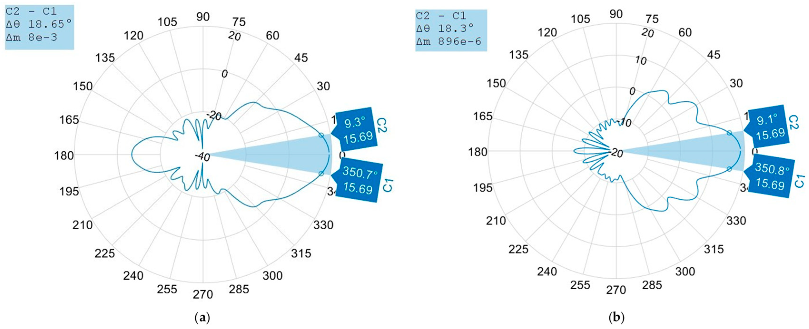
The latter pattern measurements are the determination of the antenna directivity, radiation patterns, and half-power beam widths (HPBW) in the azimuth and elevation planes at . The antenna is simulated as a perfect electric conductor (PEC) with an efficiency () value of 1 over the entire frequency range, therefore directivity and gain are interchangeable here. Figure 4 shows the directivity pattern overlayed on the horn antenna, with a maximum main lobe value of 18.69 dBi at . Figure 5 deconstructs this pattern into the azimuth and elevation planes, with similar HPBW values of 18.65° and 18.30° respectively; these are below the desired 20° threshold and comparable with commercially available horn antennas. Whilst the horn antenna was chosen for its directivity, HPBW values below 15° are not desirable as drone flight instabilities will disproportionately affect overly focused radar measurements. Non-linear human input may be mitigated through flight planning, waypoints, autopilot, and other intelligent flight features of professional and industrial drones. However, the aircraft is still subject to wind, turbulence, and atmospheric thermal gradients. HPBW values between 15° and 20° therefore satisfy the trade-off between antenna directivity and positioning sensitivity.
2.3. Fabrication
The horn antennas were fabricated in the Geotechnics laboratory and workshop of the Department of Civil and Environmental Engineering at Imperial. Two antennas were produced for simultaneous signal transmission (Tx) and reception (Rx) and are numbered as Antenna 1 and Antenna 2 throughout, according to the order of their production.
Copper was chosen as a suitable antenna fabrication material due to its high conductivity. The primary material utilised here is a 1.6 mm thick, single-sided, FR-4 material grade CCL epoxy board. Previous demonstrations have shown antennas either integrated into the substrate or lined with this material [44,45,46,47,48,49,50], with this being the first demonstration of horn antennas fabricated from the CCL itself. The board base consists of eight layers of woven glass-reinforced fabric laminate epoxy resin. This provides a lightweight and rigid structure to the antenna at a suitable thickness for dimensional stability during drone deployment. The particular substrate material does not affect the antenna performance, since the 35-µm-thick copper at the internal surfaces provides a boundary for the electromagnetic field. CCL is deemed preferable to copper sheets for achieving a lightweight component for drone deployment, given their respective material densities of 1.8 and 8.96 g/cm3 [57]. To achieve an equivalent component weight, a copper sheet thickness of approximately 0.32 mm is required, which is anticipated to provide insufficient dimensional stability for drone deployment. Furthermore, the manufacturing cost of CCL is highly competitive, being comparable to the additive manufacturing mentioned in Section 1, and considerably cheaper than copper sheet which is highly dependent on the component thickness.
Each antenna consists of nine pieces of the CCL board: five for the waveguide section and four for the flared section. These were machined from the larger CCL boards using an XYZ computer numerical control (CNC) machine and a manual guillotine. The pieces were soldered together on the internal joints using 0.7 mm multicore wire lead solder, with an approximate melting point of 183–188 °C. The first prototype showed some separation at these joints. Therefore, 1-mm-thick silver anodized aluminium was attached to the external edges of the flared section using water-resistant epoxy adhesive to support the soldered joints, with 15 mm overlap to either side. This aluminium was chosen because it is lightweight, strong, and scratch resistant. Similarly, flat aluminium pieces were secured to the connections between the waveguide and flared sections, given their relative size difference and the resulting stresses on these joints. A 1-mm diameter hole was drilled at the pre-determined input feed position. The waveguide input feed was made by soldering a brass rod into the solder cup of a 50 Ω straight flange mount SMA connector. Heat shrink tubing was applied around the solder cup to isolate the SMA core to the body of the antenna (Figure 6). The input feed penetrates the waveguide by 13.88 mm and is secured to the external waveguide face using the same epoxy adhesive.
The CCL board was chosen for being lightweight, with Antennas 1 and 2 weighing 0.49 and 0.50 kg respectively. The slight disparity is acceptable and attributed to differences in the quantity and positioning of the flat aluminium pieces (Figure 7). The combined weight of 0.99 kg is the heaviest component of the radar payload, although well within the potential payload capacity of 6 kg for the DJI Matrice 600 Pro drone.
2.4. Testing
Antenna testing was performed to compare the simulated and fabricated antenna performances. The S11, gain, radiation patterns, and beamwidths were measured in a radio frequency (RF) electromagnetic anechoic chamber using a calibrated vector network analyser (VNA).
2.4.1. Vector Network Analyser
The VNA used for the antenna measurements is the LibreVNA™. NanoVNAs provide a lower cost option for antenna measurements compared to standard laboratory VNAs; however, most have a measurement range up to 1.50 or 3.00 GHz, which is insufficient for these antennas and their operating frequencies. The LibreVNA™ was chosen because it covers the full frequency range of operation up to 6.00 GHz, with full 2-port functionality for determining all four S-parameters (S11, S12, S21, S22). The dynamic range is >95 dB to 3.00 GHz and >50 dB to 6.00 GHz [58]. The S11 is measured for both antennas. The S21 is measured for the gain and radiation pattern determination. The LibreVNA™ does not have a heatsink due to the compact design, with operating temperatures of approximately 60 °C to be expected and heat dissipated through the metal case. The potential impact of thermal drift on the antenna measurements is mitigated by restricting the operating time to 10-min intervals and installing the VNA between two aluminium heatsinks. It was observed that the surface temperature of the VNA when handled was significantly lower and the results appeared more consistent when following these mitigation procedures.
2.4.2. Anechoic Chamber
The antenna measurements were conducted in the RF Electromagnetic Laboratory in the Centre for Bio-Inspired Technology at Imperial. This 4 × 3 × 2 m anechoic shielded chamber fitted by EMV Ltd. enables low noise measurements with significantly attenuated electromagnetic levels and is calibrated for uninterrupted use between 10 MHz and 34 GHz. The chamber walls and floor are lined with a carbon-impregnated polyurethane pyramidal foam absorber material. The dielectric properties and geometry of this foam acts to resist and dissipate the electromagnetic waves, to ensure that signals are received from the signal source and not from internal reflections [59]. The central platform was rearranged to enable farfield measurements, with a maximum distance between antennas of 2.70 m and an antenna farfield distance of 1.84 m at the maximum test frequency of 6 GHz ( = 0.05 m). Discrete SMA wall sockets enable the operation of the VNA from outside the chamber, thus shielding the antenna/device under test (A/DUT) inside from electromagnetic interference. A Windows 10 laptop with an Intel® Core™ i7-4810MQ Processor at 2.80 GHz and 16 GB RAM was used to power and operate the software for the LibreVNA™.
2.4.3. S11
The VNA was calibrated with the short-open-load-through (SOLT) technique to ensure accuracy. This procedure is the one-port impedance measurements of both ports 1 and 2 using shorted, open, and 50 Ω load terminations, and the two-port transmission measurement via a coaxial cable through standard [60]. S11 measurements were then collected from 1 MHz to 6 GHz across 501 discrete frequency points for both antennas (Figure 8). This frequency range was chosen to match the simulated S11, for comparison to the WR187 and values and assessment of the bandwidth potential.
2.4.4. Gain
The three-antenna gain-transfer method outlined in the IEEE Standard Test Procedures for Antennas [61] and Balanis [62] is used to determine the realized antenna gain. The Linx ANT-W63WS2 is used as the reference antenna since it satisfies the three requirements for gain standards: (1) the antenna gain (GRef) is accurately known. GRef values are the peak gain in the edge-bent configuration at 50 MHz increments; (2) the antenna has a high degree of dimensional stability; and (3) the linear polarization of the antenna matches that of the AUT. Dipole and pyramidal horn antennas are universally accepted for use as gain standards [61]. However, the latter prohibits a cost-effective testing methodology for this scenario and thus negates the purpose of developing the low-cost horn antennas. The selected WiFi antenna is inexpensive, consists of a one-half wavelength dipole configuration, and operates with a maximum voltage standing wave ratio (VSWR) and efficiency of 1.5:1 and 89% respectively between 5.15 and 5.85 GHz. The reference antenna is connected to the Rx port (2) of the VNA. An antenna with sufficient dynamic range to transmit to the reference antenna is connected to the Tx port (1) of the VNA and placed at a farfield separation distance of 2.70 m. In this case, the horn antenna currently not being tested is used as the transmitter. The antennas are aligned in polarization and direction of maximum radiation intensity. A foam wedge and a flexible clamp are used to vertically align the transmit and receive antennas respectively. Absorbing material is located immediately behind the gain standard on the chamber door to reduce reflections impacting the illuminating field [61]. The normalized calibration is performed on the VNA to normalize the gain response to the reference antenna and produce a flat S21 graph. The reference antenna is replaced with the AUT, maintaining the exact position and alignment. The new S21 values (GRel) are recorded at 501 discrete frequency points in 2 MHz increments between 5 and 6 GHz, as relative to the reference antenna. These values are mean averaged across 24 MHz increments to capture the gain response of the typical SDR bandwidth, and to smooth the fluctuations between measurements. The antenna gain (GAUT) is determined as the sum of GRef and GRel at each frequency point, where the former is interpolated from 50 to 24 MHz, and assuming antenna reciprocity between reception and transmission:
2.4.5. Radiation Pattern
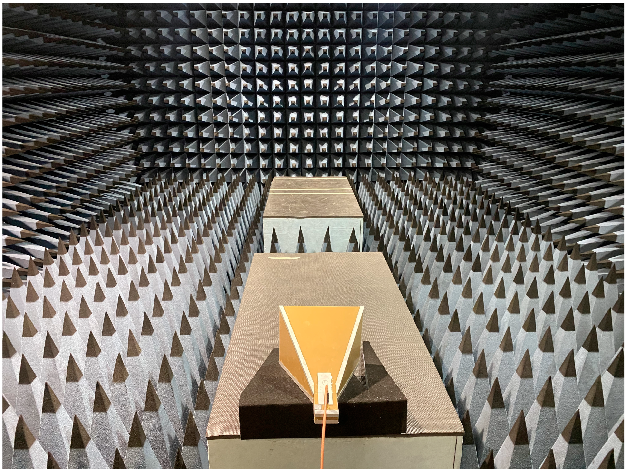
The experimental setup outlined in Section 2.4.4 is utilised for the determination of antenna radiation patterns; the gain is normalized to the reference antenna, before connecting the spare horn antenna and AUT to ports 1 (Tx) and 2 (Rx) of the VNA, respectively. The radiation pattern determination procedures outlined in [61,62,63] are followed. The receiving AUT is placed upon a turntable labelled with 10° increments. A foam wedge is used to elevate the antenna on the turntable to limit ground reflections from the plastic surface. The transmitting antenna is vertically aligned using a larger foam wedge. Both antennas maintain a constant elevation geometry throughout. The AUT is manually rotated through the entire 360° of the azimuth plane in 10° increments, with S21 measurements taken at each point to indicate the field strength; 10° is deemed feasible for accurate measurements through manual rotation, and suitable for understanding and demonstrating the antenna performances in this use case. The spherical coordinate system in which the antenna operates is mechanically defined with the AUT at the centre [61]. The frequency and polarisation are consistent throughout. Performing this experiment in an anechoic chamber is essential for limiting reflections from other surfaces that may distort the radiation pattern. Figure 9 shows the experimental setup with the AUT in the foreground oriented at 180° θ, in the complete opposite direction from the Tx antenna in the background. Rotating the AUT about the vertical axis allows the transmit antenna to illuminate it at different angles, thus determining the azimuth pattern cut. It was considered unfeasible to accurately determine the elevation pattern cut in the relatively small anechoic chamber, with the assumption that the azimuth pattern cut and beamwidth derivative are sufficient to determine the antenna directivity in combination with the gain.
2.5. Incorporation into the Drone Radar Payload
The antennas are incorporated into an aluminium payload enclosure, which attaches to the underside of the DJI Matrice 600 Pro in a modular fashion. Aluminium was chosen as a suitable material since it is a lightweight metal, which provides good strength and stability at small thicknesses. The main platform consists of a 175 × 285 × 1 mm aluminium sheet. The expansion mounting kit on the underside of the drone is removed to reveal four thread pillars which are used to mount the corners of the payload platform. Figure 10 shows the payload schematic, with annotated features described in Table 2. The antennas are secured together and to the payload for safety and redundancy. Adequate space is provided for other radar payload components, including a Raspberry Pi 4 8 GB for remote operation of the Ettus USRP E312 SDR. The payload and antennas are oriented towards the front of the drone, due to the landing gear mechanisms and legs on the sides of the drone. As the drone can move about the yaw axis of rotation, the antennas can achieve the side-looking antenna viewing geometry required for SAR with forward-mounted antennas and sideways flight, as shown in Figure 11b.
3. Results
3.1. Testing Results
3.1.1. S11
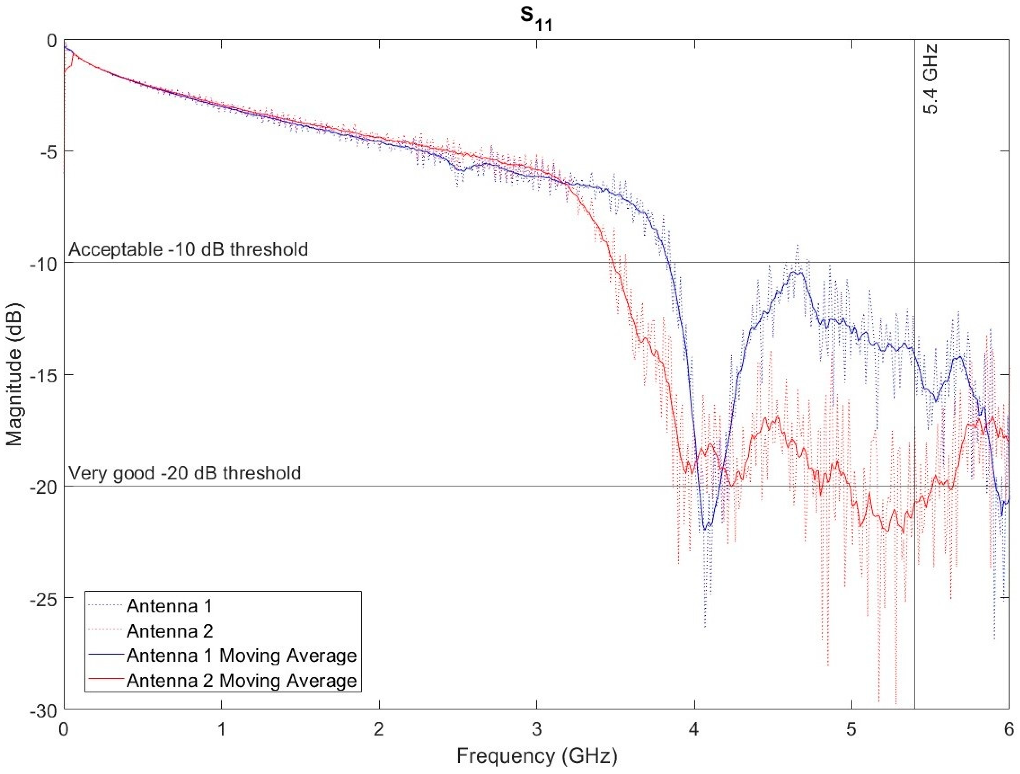
Antennas 1 and 2 have similar S11 trends from 0.00 to 3.20 GHz (≈), before passing the −10 dB (< 10% reflection loss) threshold at 3.85 and 3.57 GHz respectively (Figure 12). Values remain below −10 dB to 6.00 GHz, except for Antenna 1 briefly at 4.65 GHz. The S11 trends between the antennas are similar but offset in magnitude, with Antenna 2 typically experiencing lower values across the frequency range of interest. S11 at is −14.20 dB and −20.70 dB for Antennas 1 and 2, denoting reflection losses of 3.80% and 0.85% respectively.
3.1.2. Gain
3.1.3. Azimuth Radiation Pattern and HPBW
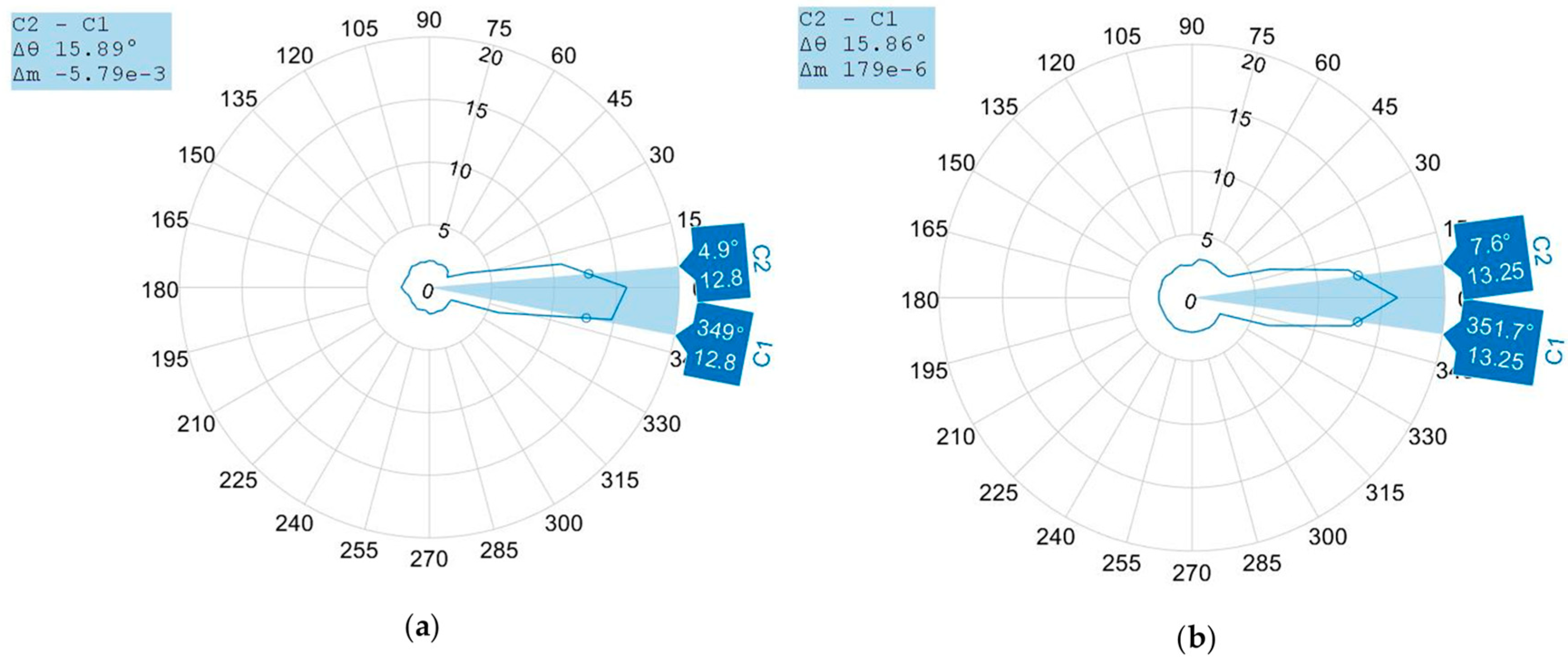
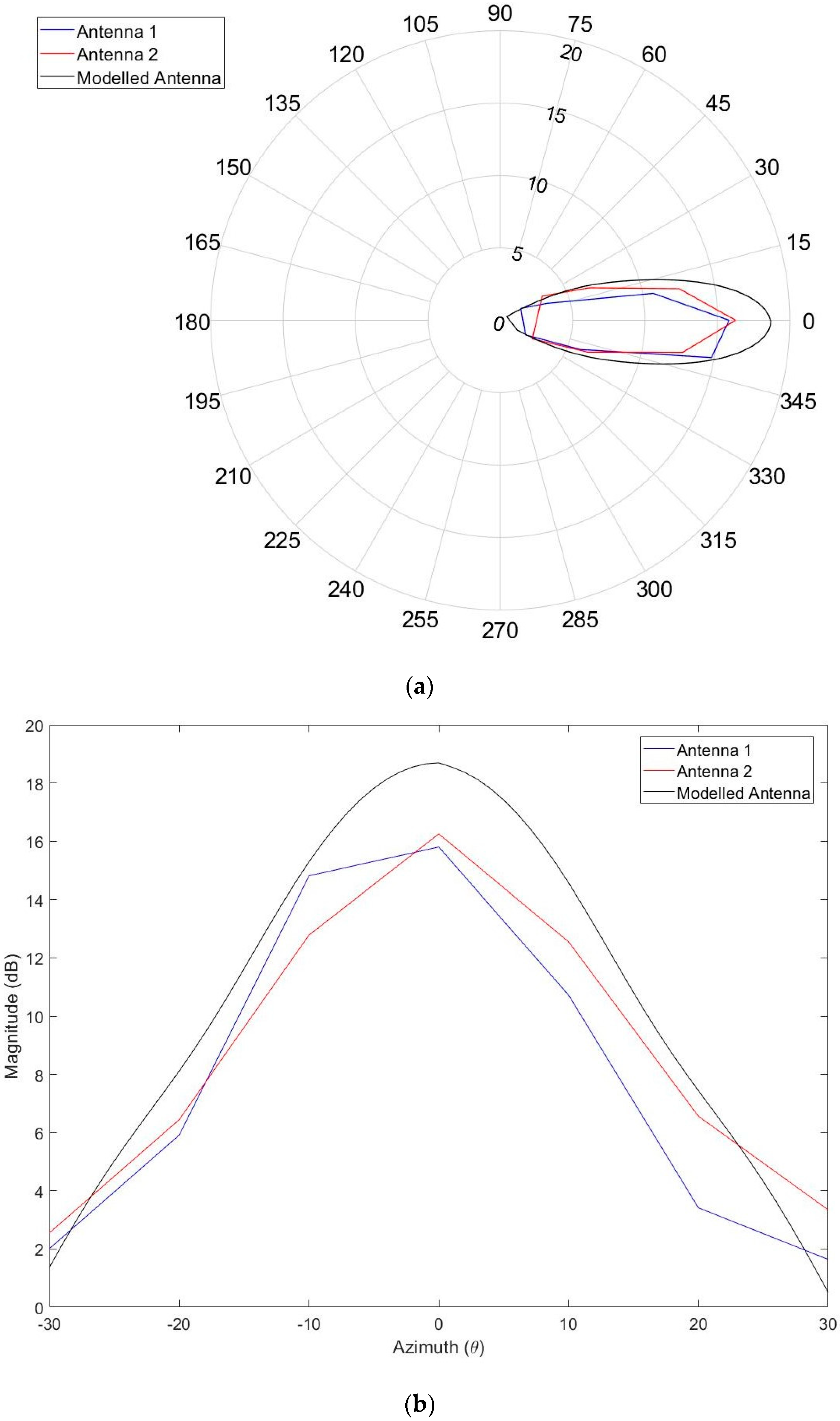
The azimuth HPBW at is 15.89° and 15.86° for Antennas 1 and 2 respectively (Figure 14). The radiation patterns are highly directive with only the main lobe identified. For Antenna 2, this is roughly symmetrical with ±3 dBi at 7.56° and 8.30° . Antenna 1 is less symmetrical, with ±3 dBi at 4.89° and 11.0° . For both antennas, the side and back lobes are amalgamated into a roughly uniform and spherical radiation pattern; for Antenna 1, between 30.20° and 328.00° with a mean average magnitude of 2.01 dBi; for Antenna 2, between 30.50° and 330.00° with a mean average magnitude of 2.73 dBi.
3.2. Drone Radar Payload
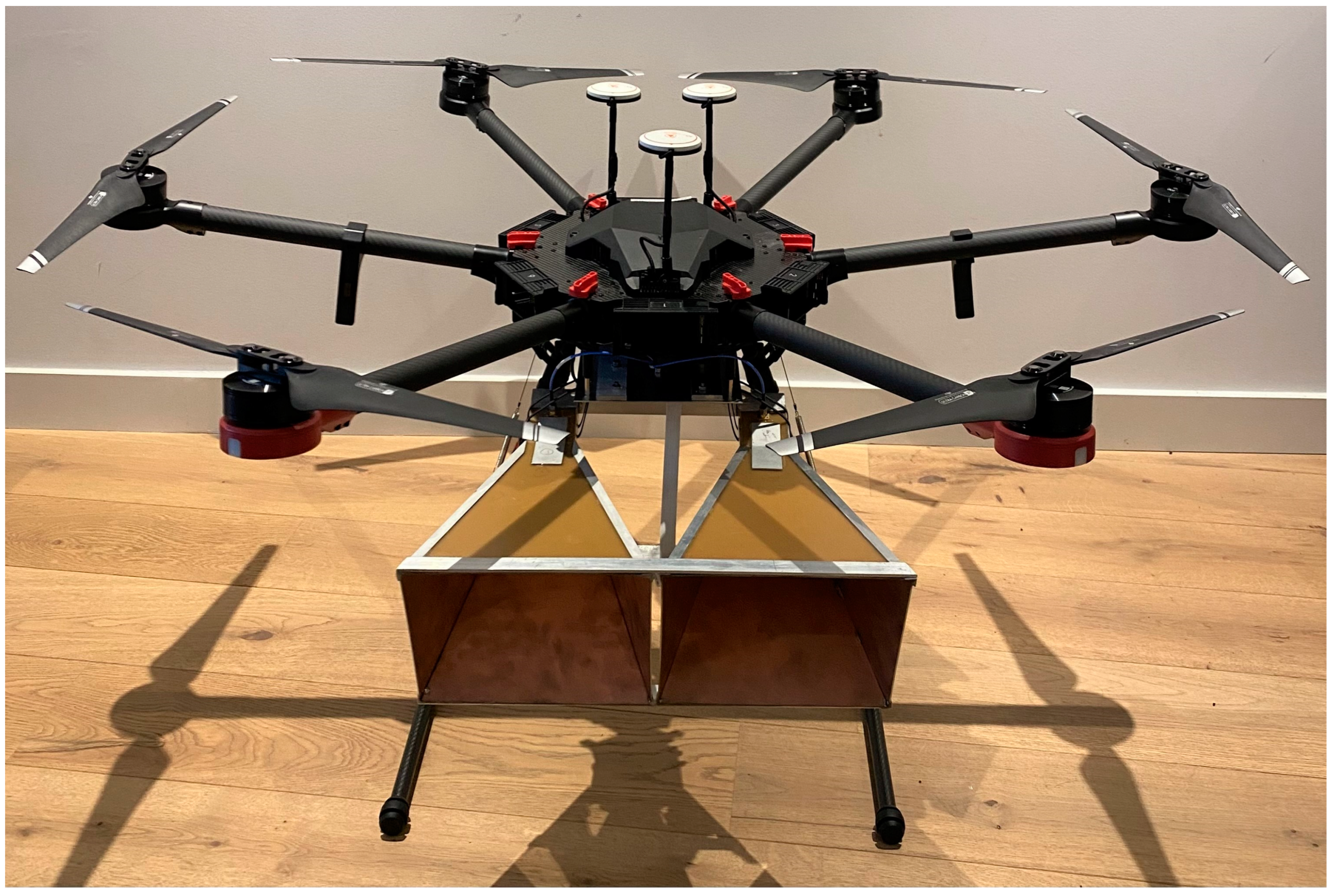
Figure 15 shows the antennas secured together and incorporated into the drone radar payload. Figure 16 shows the radar payload attached to the DJI Matrice 600 Pro. Numerous flight characterisation tests have demonstrated that the drone can maintain good stability and control with the additional payload.
4. Discussion
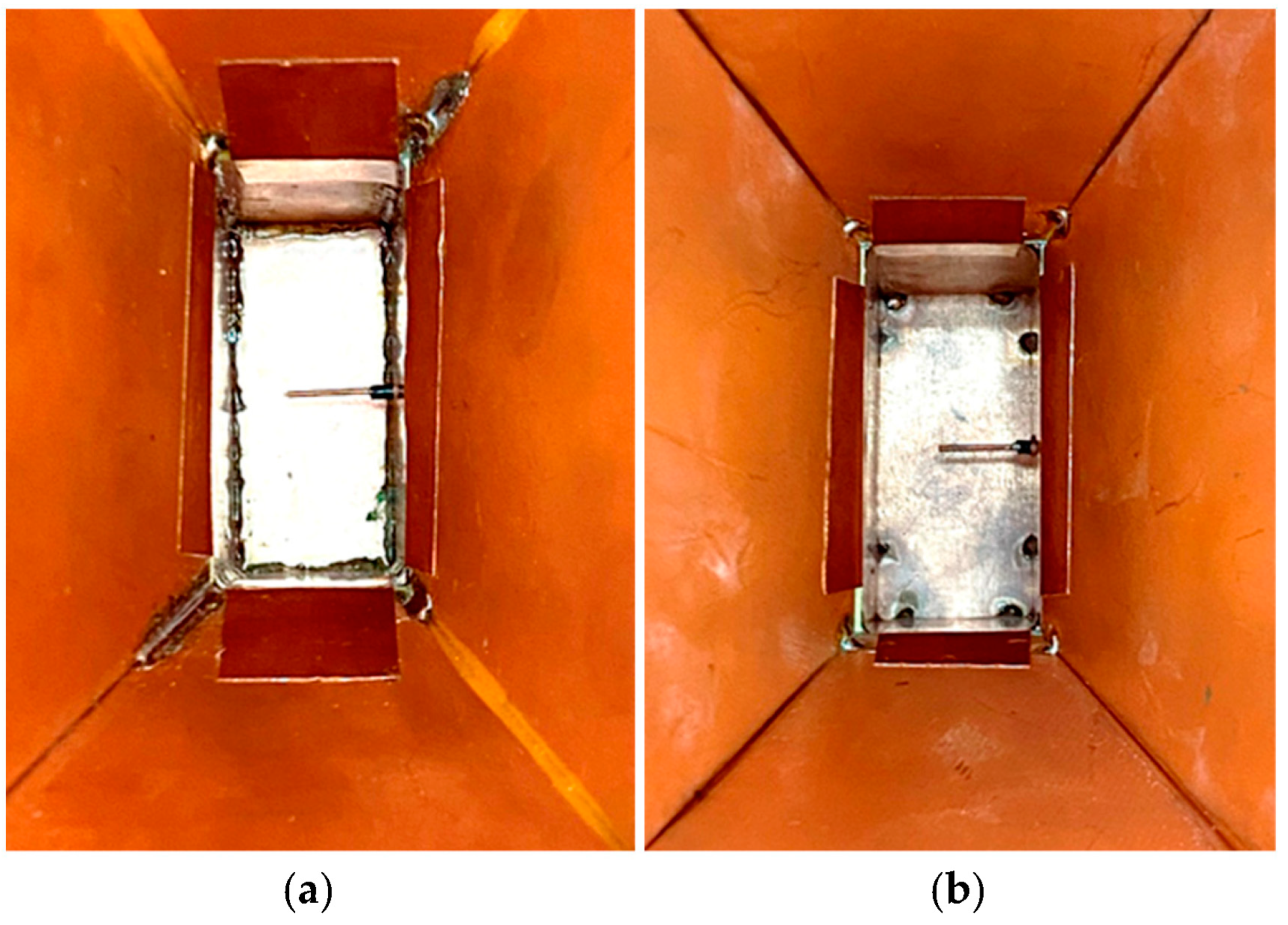
The measured S11 in relation to the typically accepted −10 dB threshold suggests that both antennas have a wide frequency bandwidth that roughly aligns with the WR187 and values of 3.95 and 5.85 GHz respectively that the horn waveguide is designed on. Reflection losses were expected to be greater in comparison to the simulated S11 due to the SDR, cable, and hardware setup. Instead, compared to the simulation, Antenna 1 performs similarly at , and Antenna 2 performs very well throughout the frequency range. It is not possible to quantitatively determine the precise contributing factors for the discrepancies between the simulated and measured S11; nevertheless, several potential justifications are provided in accordance with similar antenna studies with S11 discrepancies. This includes the simulated PEC not accounting for the CCL material properties [64], and the unique fabrication qualities and tolerances [65,66,67]. Furthermore, whilst the simulation is excited by a waveguide port, the fabricated antenna is excited by the SMA connector, which affects the contribution of connector losses [68]. The testing procedures are not considered to be an influencing factor, since the SOLT calibration ensures VNA accuracy. The S11 performance disparity between the two antennas is attributed to slight differences in their manufacturing tolerances, as bespoke, handmade components [65]. The only differing factor in their fabrication is the internal soldering patterns in the waveguide and horn aperture. Antenna 1 has an increased number of joint solders which are generally untidy, that may have increased signal reflections compared to the relatively clean spot soldering on Antenna 2 (Figure 17). Nevertheless, this disparity is deemed acceptable given that both antennas surpass the −10 dB threshold, and Antenna 2 shows very good performance surpassing −20 dB. The S11 results indicate that both antennas perform and are impedance matched well at and across the broader WR187 bandwidth, which is sufficient for the maximum instantaneous bandwidth of 56 MHz provided by the Ettus USRP E312 [52].
The GAUT at is 15.80 and 16.25 dBi for Antennas 1 and 2 respectively; this slight discrepancy is attributed to the aforementioned S11 results, where Antenna 2 has a preferable ratio of radiated to reflected power. Nevertheless, the GAUT for both antennas is below the intended and simulated values of 19 and 18.69 dBi respectively. As stated, the dimensions were optimized for 19 dBi gain, to provide leniency for manufacturing artefacts that may reduce the gain.
Whilst soldering occurs in localised spots along the internal edges, the exterior aluminium ensures that the PCB parts are fully galvanically contacted, thus preventing energy leakage contributing to the gain discrepancies.
The simulation of a PEC assumed a of 1 and thus an interchangeable directivity and gain. The CCL has inefficiencies, due to surface roughness effects and the finite copper conductivity compared to the PEC. Regarding the former, the skin depth describes the current density distribution throughout the copper conductor; this parameter decreases with increasing frequency to 0.8872 μm at . Surface roughness of the copper layer at a scale equivalent to the skin depth therefore introduces losses at these frequencies [69]. Regarding the latter, some minor conduction losses are anticipated, such as resistive and ohmic losses in the copper layer [70]. However, both are considered negligible to justify the measured gain discrepancies of 2–3 dBi.
Instead, the simulated to measured gain discrepancies at are attributed to a resonant frequency shift. Figure 13 shows that both antennas follow a similar gain trend, therefore any gain discrepancy is not due to their individual manufacturing artefacts. Both antennas perform as intended at slightly lower frequencies; for Antenna 1, gain is above 18 dBi from 5.05 to 5.22 GHz, and similarly for Antenna 2, gain is 20.87 dBi at 5 GHz and 18.69 dBi at 5.25 GHz. These results indicate a similar frequency offset impacting the gain results for both antennas, where the ideal centre frequency is around 5.1 GHz. The resonant frequency of a horn antenna is determined by the physical dimensions and the dielectric properties of the materials. Whilst the antenna and input feed are dimensionally accurate to the simulation, the brass composition of the latter has material properties that are different to the simulated PEC and the copper interior. The resonant frequency shift is therefore attributed to the 260 brass rod input feed, which has a composition of 70% copper, 30% zinc, and negligible iron and lead constituents. A lower conductivity, 28% of the International Annealed Copper Standard (IACS) [71], introduces resistance, thus increasing losses and reducing efficiency at the input feed. Furthermore, the increased skin depth of brass compared to copper increases the electrical length of the input feed, thus shifting the resonance to a lower frequency with a longer wavelength. Future iterations of the antennas will implement a copper input feed to address this.
The azimuth HPBW values of 15.89° and 15.86° are preferable to the simulated value of 18.65°, show consistent performance between the two antennas, and satisfy the requirement of values between 15° and 20° for drone radar. The asymmetry in the main lobe radiation pattern of Antenna 1 may be attributed to slight misalignments of the Tx and Rx AUT, as the resultant HPBW value is similar to Antenna 2. The sharp lines of the main lobes for both antennas are a result of manually conducting measurements at 10° increments and linearly interpolating the magnitude between points, whereas the azimuth radiation pattern was simulated at 1° increments. This effect could be mitigated by using a mechanical rotator that can automatically and precisely rotate the AUT to smaller increments. For this investigation, the data has a sufficient resolution for identifying the main lobes and HPBW from them. Since the main lobe extent for both antennas are approximately between ±30° from 0° , this angular range is compared with the simulated azimuth radiation pattern (Figure 18). The extent of the simulated main lobe with a magnitude greater than 0 dBi is also between ±30° from 0° . The differences between the simulated and measured azimuth patterns are the magnitude of the main lobe (GAUT), the angular width of the main lobe (HPBW) and the magnitude of the side and back lobes. Regarding the latter, for the simulated azimuth, there are five lobes on either side of the antenna with peak magnitudes less than −20 dBi, and one larger back lobe with a peak magnitude of −6.74 dBi. The dynamic range of the VNA was optimized to detect signals at this level [58], and the measurements were conducted in a low to zero noise environment [59]. It is therefore assumed that this difference between simulated and measured side and back lobe magnitudes is not due to any limitations of the VNA or a noise floor higher than the signal of interest. Instead, average magnitudes of 2.01 and 2.73 dBi may reflect the true signal reception at these angular ranges, either due to signal reception at the SMA connector of the waveguide section, or minor reflections caused by the plastic turntable. Despite this, the key performance indicator of antenna directivity here is the main lobe magnitude, which is 4.89 and 4.74 times greater than the mean average side and back lobe magnitudes for Antennas 1 and 2 respectively. These main lobes align well with the simulated azimuth pattern ± 30° from 0° , which, in combination with the gain results, indicates a good directivity.
These findings represent the early stages of research for the niche technological application of drone radar. To ensure reproducibility going forward, proper and consistent soldering techniques will be applied to future antenna iterations, as this was the only differing factor in their fabrication and highlighted as the source of discrepancies in the measurements.
Despite this, both antennas perform well and are deemed suitable for this use case as the performance criteria are satisfied. This includes gain exceeding 15 dBi, azimuth beamwidth between 15° and 20°, and S11 below −10 dB. These criteria were determined based upon common RF principles and equivalent metrics in other drone radar applications. Therefore, the measured antenna performances inherently verify their suitability for drone radar and InSAR applications.
5. Conclusions
We have demonstrated the design, simulation, fabrication, and testing of two horn antennas for deployment in a drone radar payload. The design process considered the size and weight requirements of drone deployment and optimized the antenna dimensions for C-band radar through an iterative process. The simulation results indicated a suitable design with good performance that was realized through CCL/PCB/FR-4 fabrication techniques. The antennas were tested in a RF electromagnetic anechoic chamber using a calibrated VNA for comparison with the simulated parameters. Despite a performance disparity which is attributed to artefacts of the manufacturing and testing processes, both antennas perform well, have a wide bandwidth of potential operation, and are suitable for deployment in the drone radar payload. Antenna measurement techniques could be improved, e.g., using a mechanical rotator or including the elevation pattern cut. However, the testing methodology outlined here is suitable for understanding and demonstrating the antenna performances in this use case.
Following their fabrication, the antennas were utilised in an in-situ laboratory investigation of the impact of soil moisture content on the phase of backscattered radar waves. Subsequently, the antennas were successfully incorporated into the modular radar payload.
The main contributions of this work include:
- The first demonstration of horn antennas fabricated from CCL, highlighting the potential for this inexpensive material to be utilised for antenna fabrication. The combination of a lightweight dielectric substrate with a smooth and conductive copper coating at a thickness of multiple skin depths produces antennas that are suitable for drone deployment, with sufficient performance metrics for our applications.
- The identification of manufacturing processes for CCL antennas that impact the performance metrics, including the internal soldering patterns and input feed material.
- The first complete overview of custom antenna production for drone radar deployment, including incorporation into the drone payload, thus demonstrating a hardware solution in the emerging field of drone SAR and InSAR research.
Author Contributions
Conceptualization, A.C.; data curation, A.C.; formal analysis, A.C.; funding acquisition, J.A.L., R.G. and P.J.M.; investigation, A.C.; methodology, A.C.; project administration, J.A.L., R.G. and P.J.M.; resources, A.C.; software, A.C.; supervision, J.A.L., R.G. and P.J.M.; validation, A.C.; visualization, A.C.; writing—original draft, A.C.; writing—review & editing, J.A.L., R.G. and P.J.M. All authors have read and agreed to the published version of the manuscript.
Funding
This research was funded by the EPSRC Centre for Doctoral Training in Nuclear Energy: Building UK Civil Nuclear Skills for Global Markets, grant number EP/L015900/1. The APC was funded by UKRI.
Institutional Review Board Statement
Not applicable.
Informed Consent Statement
Not applicable.
Data Availability Statement
The study did not report any data.
Acknowledgments
The authors acknowledge the Geotechnics technicians in the Department of Civil and Environmental Engineering at Imperial College London for their assistance in the antenna fabrication; including Prashant Hirani, Alexandros Stefanos Karapanagiotidis, Steve Ackerley, and Graham Keefe. The authors also acknowledge the assistance of Peilong Feng, for providing induction and access to the anechoic chamber at Imperial.
Conflicts of Interest
The authors declare no conflict of interest.
References
- Uys, D. InSAR: An introduction. Preview 2016, 182, 43–48. [Google Scholar] [CrossRef] [Green Version]
- Wang, Z.; Lawrence, J.; Ghail, R.; Mason, P.; Carpenter, A.; Agar, S.; Morgan, T. Characterizing Micro-Displacements on Active Faults in the Gobi Desert with Time-Series InSAR. Appl. Sci. 2022, 12, 4222. [Google Scholar] [CrossRef]
- Massonnet, D.; Rossi, M.; Carmona, C.; Adagna, F.; Peltzer, G.; Feigl, K.; Rabaute, T. The displacement field of the Landers earthquake mapped by radar interferometry. Nature 1993, 364, 138–142. [Google Scholar] [CrossRef]
- Feigl, K.; Sarti, F.; Vadon, H.; McClusky, S.; Ergintav, S.; Durland, P.; Bürgmann, R.; Rigo, A.; Massonnet, D.; Reilinger, R. Estimating slip distribution for the Izmit mainshock from coseismic GPS, ERS-1, RADARSAT and SPOT measurements. Bull. Seismol. Soc. Am. 2002, 92, 138–160. [Google Scholar] [CrossRef]
- Fielding, E.J.; Talebian, M.; Rosen, P.A.; Nazari, H.; Jackson, J.A.; Ghorashi, M.; Walker, R. Surface ruptures and building damage of the 2003 Bam, Iran, earthquake mapped by satellite synthetic aperture radar interferometric correlation. J. Geophys. Res. 2005, 110, 1–15. [Google Scholar] [CrossRef] [Green Version]
- Fattahi, H.; Amelung, F. InSAR observations of strain accumulation and fault creep along the Chaman Fault system, Pakistan and Afghanistan. Geophys. Res. Lett. 2016, 43, 8399–8406. [Google Scholar] [CrossRef] [Green Version]
- Cavalié, O.; Lasserre, C.; Doin, M.P.; Peltzer, G.; Sun, J.; Xu, X.; Shen, Z.K. Measurement of interseismic strain across the Haiyuan fault (Gansu, China), by InSAR. Earth Planet. Sci. Lett. 2008, 275, 246–257. [Google Scholar] [CrossRef]
- Aditiya, A.; Aoki, Y.; Anugrah, R.D. Surface deformation monitoring of Sinaburg volcano using multi temporal InSAR method and GIS analysis for affected area assessment. IOP Conf. Ser. Mater. Sci. Eng. 2018, 344, 012003. [Google Scholar] [CrossRef]
- Massonnet, D.; Briole, P.; Arnaud, A. Deflation of Mount Etna monitoring by spaceborne radar interferometry. Nature 1995, 375, 567–570. [Google Scholar] [CrossRef]
- Amelung, F.; Jónsson, S.; Zebker, H.; Segall, P. Widespread uplift and trap door faulting on Galápagos volcanoes observed with radar. Nature 2000, 407, 993–996. [Google Scholar] [CrossRef]
- Liu, P.; Li, Z.; Hoey, T.; Kincal, C.; Zhang, J.; Zeng, Q.; Muller, J.P. Using advanced InSAR time series techniques to monitor landslide movements in Badong of the Three Gorges region, China. Int. J. Appl. Earth Obs. Geoinf. 2013, 21, 253–264. [Google Scholar] [CrossRef]
- Bianchini, S.; Pratesi, F.; Nolesini, T.; Casagli, N. Building deformation assessment by means of persistent scatterer interferometry analysis on a landslide-affected area: The Volterra (Italy) case study. Remote Sens. 2015, 7, 4678–4701. [Google Scholar] [CrossRef] [Green Version]
- Carla, T.; Intrieri, E.; Raspini, F.; Bardi, F.; Farina, P.; Ferretti, A.; Colombo, D.; Novali, F.; Casagli, N. Perspectives on the prediction of catastrophic slope failures from satellite InSAR. Sci. Rep. 2019, 9, 14137. [Google Scholar] [CrossRef] [PubMed] [Green Version]
- Velasco, V.; Sanchez, C.; Papoutsis, I.; Antoniadi, S.; Kontoes, C.; Aifantopoulou, D.; Paralykidis, S. Ground deformation mapping and monitoring of salt mines using InSAR technology. In Proceedings of the Solution Mining Research Institute (SMRI) Fall 2017 Technical Conference, Münster, Germany, 25–26 September 2017. [Google Scholar]
- Akçin, H.; Degucci, T.; Kutoglu, H.S. Monitoring mining induced subsidence using GPS and InSAR. In Proceedings of the XXIII International FIG Congress, Munich, Germany, 8–13 October 2006. [Google Scholar]
- Milillo, P.; Giardina, G.; De Jong, M.J.; Perissin, D.; Milillo, G. Multi-temporal InSAR structural damage assessment: The London crossrail case study. Remote Sens. 2018, 10, 287. [Google Scholar] [CrossRef] [Green Version]
- Giardina, G.; Milillo, P.; De Jong, M.J.; Perissin, D.; Milillo, G. Evaluation of InSAR monitoring data for post-tunelling settlement damage assessment. Struct. Control. Health Monit. 2019, 26, e2285. [Google Scholar] [CrossRef] [Green Version]
- Bakon, M.; Perissin, D.; Lazecky, M.; Papco, J. Infrastructure Non-Linear Deformation Monitoring Via Satellite Radar Interferometry. Proc. Technol. 2014, 16, 294–300. [Google Scholar] [CrossRef] [Green Version]
- Tarchi, D.; Rudolf, H.; Luzi, G.; Chiarantini, L.; Coppo, P.; Sieber, A.J. SAR Interferometry for Structural Changes Detection: A Demonstration Test on a Dam. In Proceedings of the IEEE 1999 International Geoscience and Remote Sensing Symposium. IGARSS’99 (Cat. No. 99CH36293), Hamburg, Germany, 28 June–2 July 1999. [Google Scholar]
- Chang, L. Monitoring Civil Infrastructure Using Satellite Radar Interferometry. Doctoral Thesis, Delft University of Technology, Delft, The Netherlands, 2015. [Google Scholar]
- Cigna, F.; Banks, V.J.; Donald, A.W.; Donohue, S.; Graham, C.; Hughes, D.; McKinley, J.M.; Parker, K. Mapping Ground Instability in Areas of Geotechnical Infrastructure Using Satellite InSAR and Small UAV Surveying: A Case Study in Northern Ireland. Geosciences 2017, 7, 51. [Google Scholar] [CrossRef] [Green Version]
- Ge, D.; Wang, Y.; Zhang, L.; Xia, Y.; Wang, Y.; Guo, X. Using permanent scatterer InSAR to monitor land subsidence along High Speed Railway-the first experiment in China. ESA Spec. Publ. 2010, 677, 75. [Google Scholar]
- Hu, F.; Leijen, F.J.V.; Chang, L.; Wu, J.; Hanssen, R.F. Monitoring deformation along railway systems combining multi-temporal InSAR and LiDAR data. Remote Sens. 2019, 11, 2298. [Google Scholar] [CrossRef] [Green Version]
- Gray, P.C.; Ridge, J.T.; Poulin, S.K.; Seymour, A.C.; Schwantes, A.M.; Swenson, J.J.; Johnston, D.W. Integrating drone imagery into high resolution satellite remote sensing assessments of estuarine environments. Remote Sens. 2018, 10, 1257. [Google Scholar] [CrossRef] [Green Version]
- Casagli, N.; Frodella, W.; Morelli, S.; Tofani, V.; Ciampalini, A.; Intrieri, E.; Raspini, F.; Rossi, G.; Tanteri, L.; Lu, P. Spaceborne, UAV and ground-based remote sensing techniques for landslide mapping, monitoring and early warning. Geoenviron. Disasters 2017, 4, 9. [Google Scholar] [CrossRef]
- Donnellan, A.; Green, J.; Ansar, A.; Muellerschoen, R.; Parker, J.; Tanner, A.; Lou, Y.; Heflin, M.; Arrowsmith, R.; Rundle, J.; et al. Geodetic imaging of fault systems from airborne platforms: UAVSAR and Structure from Motion. In Proceedings of the IGARSS 2018–2018 IEEE International Geoscience and Remote Sensing Symposium, Valencia, Spain, 22–27 July 2018. [Google Scholar]
- Christiansen, M.P.; Laursen, M.S.; Jørgensen, R.N.; Skovsen, S.; Gislum, R. Designing and Testing a UAV Mapping System for Agricultural Field Surveying. Sensors 2017, 17, 2703. [Google Scholar] [CrossRef] [PubMed] [Green Version]
- Tulldahl, H.M.; Larsson, H. Lidar on small UAV for 3D mapping. In Proceedings of the Electro-Optical Remote Sensing, Photonic Technologies, and Applications VIII; and Military Applications in Hyperspectral Imaging and High Spatial Resolution Sensing II, Amsterdam, The Netherlands, 22–25 September 2014. [Google Scholar]
- Lin, Y.; Hyyppä, J.; Jaakkola, A. Mini-UAV-borne LIDAR for fine-scale mapping. IEEE Geosci. Remote Sens. Lett. 2010, 8, 426–430. [Google Scholar] [CrossRef]
- Sanz, M.; Fedorov, K.G.; Deppe, F.; Solano, E. Challenges in open-air microwave quantum communication and sensing. In Proceedings of the 2018 IEEE Conference on Antenna Measurements and Applications (CAMA), Västerås, Sweden, 3–6 September 2018. [Google Scholar]
- Deguchi, T.; Sugiyama, T.; Kishimoto, M. On the Development of Ground-Based and Drone-Borne Radar System. In Recent Research on Engineering Geology and Geological Engineering, Proceedings of the 2nd GeoMEast International Congress and Exhibition on Sustainable Civil Infrastructures, Egypt 2018—The Official International Congress of the Soil-Structure Interaction Group in Egypt (SSIGE); Wasowski, J., Dijkstra, T., Eds.; Springer: Cham, Switzerland, 2018; pp. 115–122. [Google Scholar]
- Deguchi, T.; Sugiyama, T.; Kishimoto, M. Development of SAR system installable on a drone. In Proceedings of the EUSAR 2021—13th European Conference on Synthetic Aperture Radar, Online, 29 March–1 April 2021. [Google Scholar]
- Li, C.J.; Ling, H. Synthetic Aperture Radar Imaging Using a Small Consumer Drone. In Proceedings of the 2015 IEEE International Symposium on Antennas and Propagation & USNC/URSI National Radio Science Meeting, Vancouver, BC, Canada, 19–24 July 2015. [Google Scholar]
- Li, C.J.; Ling, H. High-Resolution, Downward-Looking Radar Imaging Using a Small Consumer Drone. In Proceedings of the 2016 IEEE International Symposium on Antennas and Propagation (APSURSI), Fajardo, PR, USA, 26 June–1 July 2016. [Google Scholar]
- Deguchi, T.; Sugiyama, T.; Kishimoto, M. R&D of drone-borne SAR system. Int. Arch. Photogramm. Remote Sens. Spat. Inf. Sci. 2019, 42, 263–267. [Google Scholar]
- Moreira, L.; Castro, F.; Góes, J.A.; Bins, L.; Teruel, B.; Fracarolli, J.; Castro, V.; Alcântara, M.; Oré, G.; Luebeck, D.; et al. A drone-borne multiband DInSAR: Results and applications. In Proceedings of the 2019 IEEE Radar Conference (RadarConf), Boston, MA, USA, 22–26 April 2019. [Google Scholar]
- Moreira, L.; Lübeck, D.; Wimmer, C.; Castro, F.; Góes, J.A.; Castro, V.; Alcântara, M.; Oré, G.; Oliveira, L.P.; Bins, L.; et al. Drone-Borne P-Band Single-Pass InSAR. In Proceedings of the 2020 IEEE Radar Conference (RadarConf20), Florence, Italy, 21–25 September 2020. [Google Scholar]
- Oré, G.; Alcântara, M.S.; Góes, J.A.; Oliveira, L.P.; Yepes, J.; Teruel, B.; Castro, V.; Bins, L.S.; Castro, F.; Luebeck, D.; et al. Crop Growth Monitoring with Drone-Borne DInSAR. Remote Sens. 2020, 12, 615. [Google Scholar] [CrossRef] [Green Version]
- Luebeck, D.; Wimmer, C.; Moreira, L.F.; Alcântara, M.; Oré, G.; Góes, J.A.; Oliveira, L.P.; Teruel, B.; Bins, L.S.; Gabrielli, L.H.; et al. Drone-Borne Differential SAR Interferometry. Remote Sens. 2020, 12, 778. [Google Scholar] [CrossRef] [Green Version]
- Hossain, A.; Wagner, S.; Pancrazio, S.; Pham, A.V. A Compact Low-Cost and Lightweight 3-D Printed Horn Antenna for UWB Systems. In Proceedings of the 2021 IEEE International Symposium on Antennas and Propagation and USNC-URSI Radio Science Meeting (APS/USRI), Singapore, 4–10 December 2021. [Google Scholar]
- Alias, N.A.; Shaharum, S.M.; Karim, M.S.A. Design of a 3D Printed UWB Antenna for a Low-Cost Wireless Heart and Respiration Rate Monitoring. In Proceedings of the IOP Conference Series: Materials Science and Engineering, Penang, Malaysia, 17–18 April 2020. [Google Scholar]
- Carkaci, M.E.; Secmen, M. The Prototype of a Wideband Ku-Band Conical Corrugated Horn Antenna with 3-D Printing Technology. Adv. Electromagn. 2019, 8, 39–47. [Google Scholar] [CrossRef]
- Garcia, C.R.; Rumpf, R.C.; Tsang, H.H.; Barton, J.H. Effects of extreme surface roughness on 3D printed horn antenna. Electron. Lett. 2013, 49, 734–736. [Google Scholar] [CrossRef]
- Chen, Z.N.; Qing, X.; Sun, M.; Gong, K.; Hong, W. 60-GHz antennas on PCB. In Proceedings of the 8th European Conference on Antennas and Propagation (EuCAP 2014), The Hague, The Netherlands, 6–11 April 2014. [Google Scholar]
- Walbeoff, A.; Langley, R.J. Multiband PCB antenna. IEE Proc.-Microw. Antennas Propag. 2005, 152, 471–475. [Google Scholar] [CrossRef]
- Ren, W.; Deng, J.Y.; Chen, K.S. Compact PCB monopole antenna for UWB applications. J. Electromagn. Waves Appl. 2007, 21, 1411–1420. [Google Scholar] [CrossRef]
- Ghassemi, N.; Wu, K. Millimeter-wave integrated pyramidal horn antenna made of multilayer printed circuit board (PCB) process. IEEE Trans. Antennas Propag. 2012, 60, 4432–4435. [Google Scholar] [CrossRef]
- Wu, Q.; Scarborough, C.P.; Martin, B.G.; Shaw, R.K.; Werner, D.H.; Lier, E.; Wang, X. A Ku-Band Dual Polarization Hybrid-Mode Horn Antenna Enabled by Printed-Circuit-Board Metasurfaces. IEEE Trans. Antennas Propag. 2013, 61, 1089–1098. [Google Scholar] [CrossRef]
- Lashab, M.; Hraga, H.I.; Abd-Alhameed, R.A.; Zebiri, C.; Benabdelaziz, F.; Jones, S.M.R. Horn Antennas Loaded with Metamaterial for UWB Applications. In Proceedings of the Progress In Electromagnetics Research Symposium Proceedings, Marrakesh, Morocco, 20–23 March 2011. [Google Scholar]
- Lashab, M.; Zebiri, C.; Benabdelaziz, F.; Jan, N.A.; Abd-Alhameed, R.A. Horn antennas loaded with metamaterial for Ku band application. In Proceedings of the 2014 International Conference on Multimedia Computing and Systems (ICMCS), Marrakesh, Morocco, 14–16 April 2014. [Google Scholar]
- Balanis, C.A. Horn Antennas. In Antenna Theory: Analysis and Design, 4th ed.; Balanis, C.A., Ed.; John Wiley & Sons, Inc.: Hoboken, NJ, USA, 2016; pp. 719–782. [Google Scholar]
- USRP E312. Available online: https://www.ettus.com/all-products/usrp-e312/ (accessed on 20 February 2023).
- Matrice 600 Pro. Available online: https://www.dji.com/uk/matrice600-pro (accessed on 20 February 2023).
- Instrument Payload. Available online: https://sentinels.copernicus.eu/web/sentinel/missions/sentinel-1/instrument-payload (accessed on 20 February 2023).
- WR187|WG12|R48—Rectangular Waveguide Size. Available online: https://www.everythingrf.com/tech-resources/waveguides-sizes/wr187 (accessed on 20 February 2023).
- Balanis, C.A. Linear Wire Antennas. In Antenna Theory: Analysis and Design, 4th ed.; Balanis, C.A., Ed.; John Wiley & Sons, Inc.: Hoboken, NJ, USA, 2016; pp. 145–234. [Google Scholar]
- Copper Clad Boards. Available online: https://uk.rs-online.com/web/c/esd-control-cleanroom-pcb-prototyping/prototyping-boards/copper-clad-boards/ (accessed on 20 February 2023).
- LibreVNA 2 Ports Full VNA 100 kHz–6 GHz. Available online: https://eleshop.eu/librevna-2-ports-full-vna-100khz-6ghz.html (accessed on 20 February 2023).
- Electromagnetics Laboratory. Available online: https://www.imperial.ac.uk/bio-inspired-technology/facilities/em-lab/ (accessed on 2 March 2023).
- Short-Open-Load-Through (SOLT) Calibration. Available online: https://www.ni.com/docs/en-US/bundle/ni-vna/page/vnahelp/calibration_solt.html (accessed on 20 February 2023).
- The Institute of Electrical and Electronic Engineers, Inc. (IEEE) IEEE Standard Test Procedures for Antennas. In ANSI/IEEE Std 149-1979 (Revision of IEEE Std 149-1965); The Institute of Electrical and Electronic Engineers, Inc.: New York, NY, USA, 1979; pp. 1–144. [Google Scholar]
- Balanis, C.A. Antenna Measurements. In Antenna Theory: Analysis and Design, 4th ed.; Balanis, C.A., Ed.; John Wiley & Sons, Inc.: Hoboken, NJ, USA, 2016; pp. 981–1026. [Google Scholar]
- Alkaraki, S.; Gao, Y.; Torrico, M.O.M.; Stremsdoerfer, S.; Gayets, E.; Parini, C. Performance comparison of simple and low cost metallization techniques for 3D printed antennas at 10 GHz and 30 GHz. IEEE Access 2018, 6, 64261–64269. [Google Scholar] [CrossRef]
- Rahayu, Y.; Hilmi, M.F.; Wahyu, Y. Stair-Hexagonal Slot Antenna with Coplanar Waveguide Technique for Biomedical Applications. Int. J. Integr. Eng. 2000, 12, 181–188. [Google Scholar] [CrossRef]
- El-Nawawy, M.; Allam, A.M.M.A.; Ghoneima, M. Design and fabrication of W-band SIW horn antenna using PCB process. In Proceedings of the 2013 1st International Conference on Communications, Signal Processing, and their Applications (ICCSPA), Sharjah, United Arab Emirates, 12–14 February 2013. [Google Scholar]
- Midtbøen, V.; Kjelgård, K.G.; Lande, T.S. 3D printed horn antenna with PCB microstrip feed for UWB radar applications. In Proceedings of the 2017 IEEE MTT-S International Microwave Workshop Series on Advanced Materials and Processes for RF and THz Applications (IMWS-AMP), Pavia, Italy, 20–22 September 2017. [Google Scholar]
- Singh, S.K.; Sharan, T.; Singh, A.K. Investigating the S-parameter (|S 11|) of CPW-fed antenna using four different dielectric substrate materials for RF multiband applications. AIMS Electron. Electr. Eng. 2022, 6, 198–222. [Google Scholar] [CrossRef]
- Haque, M.A.; Sarker, N.; Sawaran Singh, N.S.; Rahman, M.A.; Hasan, M.N.; Islam, M.; Zakariya, M.A.; Paul, L.C.; Sharker, A.H.; Abro, G.E.M.; et al. Dual Band Antenna Design and Prediction of Resonance Frequency Using Machine Learning Approaches. Appl. Sci. 2022, 12, 10505. [Google Scholar] [CrossRef]
- Kirley, M.P.; Booske, J.H. Terahertz conductivity of copper surfaces. IEEE Trans. Terahertz Sci. Technol. 2015, 5, 1012–1020. [Google Scholar] [CrossRef]
- Chen, Q.; Ozawa, K.; Yuan, Q.; Sawaya, K. Antenna Characterization for Wireless Power-Transmission System Using Near-Field Coupling. IEEE Antennas Propag. Mag. 2012, 54, 108–116. [Google Scholar] [CrossRef]
- 260 Brass: A Guide. Available online: https://www.sequoia-brass-copper.com/brass/cartridge-yellow-brass/ (accessed on 21 February 2023).
Figure 1.
Antenna waveguide schematic and dimensions (mm): (a) XY-plane view; (b) YZ-plane view.

Figure 2.
Horn antenna dimensions schematic: (a) YZ-plane view; (b) XZ-plane view.

Figure 3.
Simulated S11 results from 1 MHz to 6 GHz, with −14.448 dB at (5.40 GHz).

Figure 4.
Simulated antenna directivity pattern with antenna overlay and a maximum value of 18.69 dBi at (5.40 GHz).
Figure 4.
Simulated antenna directivity pattern with antenna overlay and a maximum value of 18.69 dBi at (5.40 GHz).

Figure 5.
Simulated antenna beamwidths, with a maximum directivity of 18.69 dBi at f0 (5.40 GHz), in the: (a) Azimuth-plane (Azimuth 1°–360°, Elevation 0°); (b) Elevation-plane (Azimuth 0°, Elevation 1°–360°). Azimuth and Elevation HPBW values (Δθ) of (a) 18.65° and (b) 18.30° respectively, calculated as C2-C1.

Figure 6.
Soldered monopole schematic with numbered components and dimensions (mm).

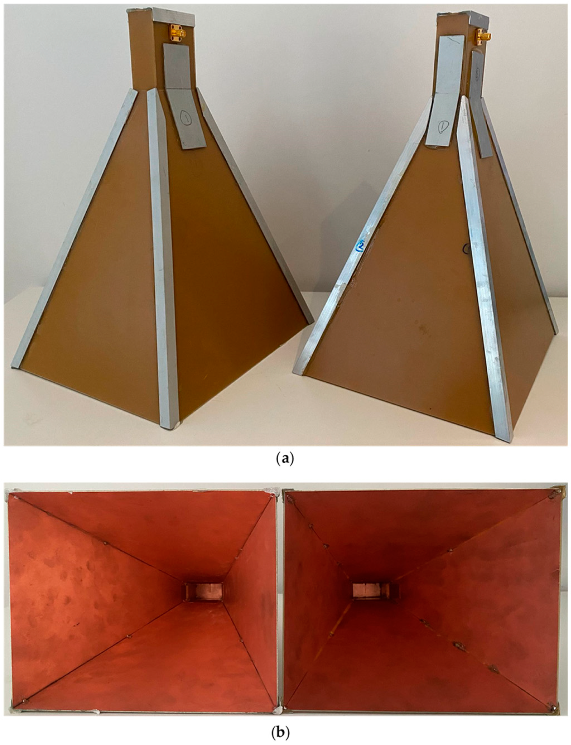
Figure 7.
Photographs of the CCL horn antennas: (a) external view; (b) internal view.

Figure 8.
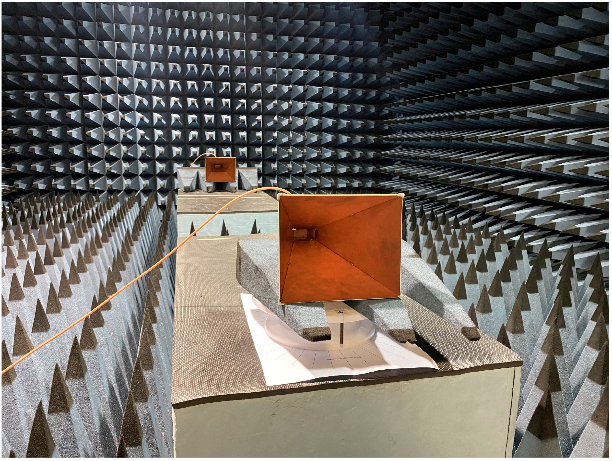
Antenna 1 S11 experimental setup in the anechoic chamber.

Figure 9.
Radiation pattern experimental setup in the anechoic chamber. Receiving Antenna 1 (foreground) upon a foam wedge and modified turntable with polar plot. Transmitting Antenna 2 upon a larger foam wedge (background) at a farfield distance of 2.70 m. Antenna 1 is positioned at 180° θ from Antenna 2.

Figure 10.
Drone radar payload schematic with annotated dimensions (mm) and annotated features described in Table 2: (a) top-view; (b) bottom-view.
Figure 10.
Drone radar payload schematic with annotated dimensions (mm) and annotated features described in Table 2: (a) top-view; (b) bottom-view.

Figure 11.
Antenna orientation with respect to the drone orientation and direction of flight, to achieve a side-looking viewing geometry of a target (a) forwards flight, with side-mounted antennas; (b) sideways flight, with forward-mounted antennas.
Figure 11.
Antenna orientation with respect to the drone orientation and direction of flight, to achieve a side-looking viewing geometry of a target (a) forwards flight, with side-mounted antennas; (b) sideways flight, with forward-mounted antennas.

Figure 12.
S11 results for Antenna 1 (blue) and 2 (red) from 0.00 to 6.00 GHz, with lines at x = 5.40 GHz (), y = −10 dB (acceptable threshold), and y = −20 dB (very good threshold). Dotted lines are measured S11 values at 501 frequency points from 1 MHz to 6.00 GHz. Solid lines are moving mean averages with a window length of 9 measurements (0.10 GHz). S11 at is −14.20 dB and −20.70 dB for Antennas 1 and 2 respectively.

Figure 13.
Gain results for Antenna 1 (blue) and 2 (red) between 5.00 and 6.00 GHz, with line at x = 5.40 GHz (). Dotted lines are measured GRel values. Solid lines (GAUT) are the sum of GRef (black) and GRel at each frequency point. GAUT at is 15.80 and 16.25 dBi for Antennas 1 and 2, respectively.

Figure 14.
Azimuth radiation pattern results (Azimuth 1°–360°, Elevation 0°), with maximum directivities of 15.80 and 16.25 dBi at (5.40 GHz) for (a) Antenna 1; (b) Antenna 2, respectively. Azimuth HPBW values ( ) of 15.89° (a) and 15.86° (b) respectively, calculated as C2-C1.
Figure 14.
Azimuth radiation pattern results (Azimuth 1°–360°, Elevation 0°), with maximum directivities of 15.80 and 16.25 dBi at (5.40 GHz) for (a) Antenna 1; (b) Antenna 2, respectively. Azimuth HPBW values ( ) of 15.89° (a) and 15.86° (b) respectively, calculated as C2-C1.

Figure 15.
Drone radar payload, with the CCL horn antennas, Ettus USRP E312 SDR and 3D printed connection stabiliser, and Raspberry Pi 4 (on the back).
Figure 15.
Drone radar payload, with the CCL horn antennas, Ettus USRP E312 SDR and 3D printed connection stabiliser, and Raspberry Pi 4 (on the back).

Figure 16.
Drone radar payload attached to the DJI Matrice 600 Pro.

Figure 17.
Internal waveguide photographs of (a) Antenna 1, with untidy soldering; (b) Antenna 2, with tidy soldering.
Figure 17.
Internal waveguide photographs of (a) Antenna 1, with untidy soldering; (b) Antenna 2, with tidy soldering.

Figure 18.
Azimuth radiation pattern main lobe results (Azimuth 330°–30°, Elevation 0°) for Antenna 1 (blue) and Antenna 2 (red), with simulated azimuth radiation pattern main lobe at the same angular range (black): (a) polar pattern; (b) magnitude plot.
Figure 18.
Azimuth radiation pattern main lobe results (Azimuth 330°–30°, Elevation 0°) for Antenna 1 (blue) and Antenna 2 (red), with simulated azimuth radiation pattern main lobe at the same angular range (black): (a) polar pattern; (b) magnitude plot.


Table 1.
Antenna dimensions.
| Parameter | Length (mm) |
|---|---|
| 47.55 | |
| 22.15 | |
| 220.58 | |
| 169.42 | |
| 214.53 | |
| 214.53 | |
| 260.93 | |
| 294.89 |
Table 2.
Descriptions of annotated drone radar payload features in Figure 10.
Table 2.
Descriptions of annotated drone radar payload features in Figure 10.
| Annotation in Figure 10 | Feature | Description |
|---|---|---|
| A | Aluminium sheet | Main platform of the payload enclosure. 175 × 285 × 1 mm aluminium sheet. |
| B | Strap | Heavy-duty elasticated strap with silicone grips, to secure the Raspberry Pi to the underside of the aluminium sheet. |
| C | E312 | Mounting position for the Ettus USRP E312 and connection stabiliser. |
| D | Aluminium reinforcements | Two 32 × 285 × 6 mm aluminium pieces for reinforcement, with 4 screws. |
| E | Mounting holes | Mounting holes for screws, which align with the thread pillars on the underside of the DJI Matrice 600 Pro. |
| F | Cable ties | Holes with cable ties for securing the platform and antenna waveguides together. |
| G | Aluminium angle | 19 × 278 × 2 mm aluminium angle, connecting the platform and antenna waveguides, with three screws. Red boxes at the screw locations denote the position of three 19 × 19 × 24 mm aluminium blocks with 15° faces installed between the aluminium sheet and perpendicular aluminium angle, to achieve the desired viewing angle. |
| H | Antennas | CCL horn antennas. |
| I | Antenna braces | 19 × 355 × 2 mm aluminium antenna brace. |
| J | Two 19 × 450 × 2 mm aluminium antenna braces. | |
| K | Raspberry Pi | Raspberry Pi mounting case position. |
| L | E312 mount | Screw holes that align with the E312 mounting holes. |
Table 3.
Gain results at (5.40 GHz) for Antennas 1 and 2, with GRef, GRel, and GAUT (dBi) values used in Equation (19).
Table 3.
Gain results at (5.40 GHz) for Antennas 1 and 2, with GRef, GRel, and GAUT (dBi) values used in Equation (19).
| AUT | GRef (dBi) | GRel (dBi) | GAUT (dBi) | ||
|---|---|---|---|---|---|
| Antenna 1 | 2.40 | + | 13.40 | = | 15.80 |
| Antenna 2 | 13.85 | = | 16.25 |
Disclaimer/Publisher’s Note: The statements, opinions and data contained in all publications are solely those of the individual author(s) and contributor(s) and not of MDPI and/or the editor(s). MDPI and/or the editor(s) disclaim responsibility for any injury to people or property resulting from any ideas, methods, instructions or products referred to in the content. |
© 2023 by the authors. Licensee MDPI, Basel, Switzerland. This article is an open access article distributed under the terms and conditions of the Creative Commons Attribution (CC BY) license (https://creativecommons.org/licenses/by/4.0/).
Share and Cite
MDPI and ACS Style
Carpenter, A.; Lawrence, J.A.; Ghail, R.; Mason, P.J. The Development of Copper Clad Laminate Horn Antennas for Drone Interferometric Synthetic Aperture Radar. Drones 2023, 7, 215. https://doi.org/10.3390/drones7030215
AMA Style
Carpenter A, Lawrence JA, Ghail R, Mason PJ. The Development of Copper Clad Laminate Horn Antennas for Drone Interferometric Synthetic Aperture Radar. Drones. 2023; 7(3):215. https://doi.org/10.3390/drones7030215
Chicago/Turabian StyleCarpenter, Anthony, James A. Lawrence, Richard Ghail, and Philippa J. Mason. 2023. "The Development of Copper Clad Laminate Horn Antennas for Drone Interferometric Synthetic Aperture Radar" Drones 7, no. 3: 215. https://doi.org/10.3390/drones7030215