Article

Evaluation of an Innovative Rosette Flight Plan Design for Wildlife Aerial Surveys with UAS

1
TERRA Teaching and Research Centre [Forest Is Life], Gembloux Agro-Bio Tech, University of Liège, Passage des Déportés 2, 5030 Gembloux, Belgium
2
Modelisation & Development Department, Gembloux Agro-Bio Tech, University of Liège, Passage des Déportés 2, 5030 Gembloux, Belgium
*
Author to whom correspondence should be addressed.
Drones 2023, 7(3), 208; https://doi.org/10.3390/drones7030208
Submission received: 31 January 2023 / Revised: 15 March 2023 / Accepted: 16 March 2023 / Published: 17 March 2023
(This article belongs to the Special Issue Drones in the Wild)

Abstract

:
(1) Regular wildlife abundance surveys are a key conservation tool. Manned aircraft flying transects often remain the best alternative for counting large ungulates. Drones have cheaper and safer logistics, however their range is generally too short for large-scale application of the traditional method. Our paper investigates an innovative rosette flight plan for wildlife census, and evaluates relevance of this sampling protocol by comparing its statistical performance with transects, based on numerical simulations. (2) The UAS flight plan consisted in two rosettes of 6 triangular “petals” spread across the survey area, for a theoretical sampling rate of 2.95%, as opposed to a 20.04% classic sampling protocol with systematic transects. We tested the logistics of our survey design in Garamba National Park. We then modeled theoretical population distributions for both antelopes and buffaloes. We calculated animal densities in the simulated footprints of the theoretical rosette and transect flight plans. We also tested aggregating results for 2, 3 and 4 repetitions of the same rosette flight plan to increase the sampling rate. (3) Simulation results showed that the coefficient of variation associated with density estimates decreases with the number of repetitions of the rosette flight plan, and aggregating four repetitions is enough to give antelope densities with acceptable accuracy and precision while staying at a lower sampling rate. Buffalo densities displayed much higher variability and it shows the significant impact of gregariousness on density estimate accuracy and precision. (4) The method was found to be inappropriate for highly aggregative species but efficient for species that disperse widely and more randomly in their environment. Logistics required to perform a full survey in the field remain time- and resources-intensive. Therefore, we recommend it for remote parks facing difficulties to organize manned aerial counts. Lower costs and developments such as solar UASs offer interesting future perspectives.

1. Introduction

Natural ecosystem conservation requires adaptive management that cannot be achieved without key elements such as regular wildlife abundance surveys [1]. In large areas, aerial surveys with light aircraft generally remain the best alternative for counting large mammals as they can cover large area in a short time, and offer a good perspective on the animal populations [1,2]. However, such surveys present a lot of challenges inherent to plane logistics. They are particularly hard to implement in the large protected areas of developing countries where finding appropriate aircraft and fuel, and qualified and trained pilots, is difficult. The only possible choice is often to rent and import the material from another country. Implementation costs of these operations are very high, and financial support from external donors is generally necessary and unpredictable making long-term monitoring strategies difficult to plan [3,4,5,6]. In many places, natural protected areas are very isolated. Maintaining airstrips in these remote places is extremely challenging and security standards are also very difficult to meet. The safety risks are also very high for operators. Wildlife census pilots have to fly at very low altitude [usually around under 350 feet], which represents an additional life-threatening risk [7,8]. The management context of many protected areas in Sub-Saharan Africa is also often subject to violent conflicts. Pilots and passengers flying low become particularly vulnerable targets for armed fighters who inhabit many of the parks where they seek hiding places, living of the resources and traffics [9].
In this context, drones (or unmanned aircraft systems, UASs) have increasingly become relevant in wildlife monitoring [3,7,10,11,12]. UASs exhibit high spatial and temporal resolution, lower operational costs and easier logistics and manipulation than manned aircraft. UASs can also fly low while being safer and less intrusive [3,7,13]. The images and videos they produce constitute systematic and permanent data, which can be archived and further reviewed by other individuals [12,14]. Finally, it can embark various other sensors, such as bioacoustics recording platforms [15,16] or radio telemetry receivers [17]. The use of lightweight UASs in wildlife monitoring may therefore be a viable an innovative alternative to traditional methods [7,12,18,19].
UASs offer many possibilities in terms of flight planning thanks to their greater maneuverability and logistical advantages [20,21]. However, most wildlife counts using drones have been inspired by either grid designs or the classic systematic transects used by manned aircraft for large scale surveys [10,12,19,22]. The UAS transect/grid methods have been widely used and proved efficient to do total counts of small dense populations, such as for bird colonies, hippo schools, shark congregations, herds and groups monitoring, … with both fixed-wings and multicopters [11,23,24,25,26,27,28]. Generally, the area surveyed is not more than a few squared kilometers and can be covered completely in one flight. In the case of free ranging animal populations spread over large territories, such as large ungulates or marine mammals, authors mostly tended to reproduce the well-known validated sampling methods based on transects, often using fixed-wings, which generally have a greater flight endurance than multicopters. However, the transect method seems to have reached its limit when it comes to perform routine large-scale drone counts and provide general abundance data [7,12,29,30]. Vermeulen et al. [31] were the first to estimate densities of a large terrestrial herbivore (Loxodonta africana) flying transects with a small drone in Burkina Faso, but were limited by the endurance and abundance results remained anecdotal. More recently, Yang et al. [32] and Guo et al. [33] conducted a census of kiang (Equus kiang) and Tibetan gazelle (Procarpa picticaudata) as well as grazing livestock in China. However, their survey focused on specific, small-size areas. The same can be said of [34]: they obtained good results counting deer with a thermal camera but their systematic transects covered a relatively small fenced research facility. Ref. [35] covered a larger area flying with a long-range (>50 km operating range) UAS to count macropods in the Australian bush. However, compared to the traditional helicopter count, the UAS was only able to survey over half of the 320 km, providing limited results. Indeed, the generally short flight endurance of small UASs is still too limited to follow the numerous long transects needed to reproduce traditional systematic aerial survey sampling plans and cover large areas, such as African protected areas (often several thousands square kilometers) [7,12,22]. The time lost travelling kilometers between effective survey strips end points can also represent a great percentage of UASs flight routes. Ref. [36] already proposed a zigzag transects method to avoid wasting that flight time during traditional censuses, but its use is of marginal help in the case of drone censuses. Furthermore, the operation radius of small UASs is generally around 15–20 km and reproducing traditional aerial survey designs would bring the plane outside its radio communication and control range capabilities most of the time, bringing a new set of operational issues [12]. The problem of limited, hard to reach, suitable take-off and landing sites can be equally challenging, especially for fixed-wing UASs [19]. Wasting flight time coming back after completing a remote flight plan also hinders efficient UAS wildlife surveys. It is therefore important to take advantage of maximal operation radius and suitable take-off sites to minimize useless run-arounds by UASs. Indeed, a lot of energy and flight time can be lost in those moments where no valuable data are taken. These limitations have resulted in most studies focusing on detection probabilities and various factors influencing it, while very few produced large-scale abundance data comparable with former surveys [12,13,37,38].
In order to make the recent technology fully operational for wider game count applications and capable of efficiently replacing or complementing manned aerial surveys for large ungulates, the aforementioned issues must be addressed. Primarily, the limitation of the relatively short range, and subsequently the total area potentially surveyed, needs to be resolved differently. Indeed, a compromise must be found between costs and logistics, and UASs capacities. Most drones offer the flexibility to follow different and more complex flight plans than transects, but few attempts have been made to adapt counting strategies. Such developments have likely been impaired by a lack of appropriate validated sampling and statistical methods [13,22], as methods for surveying large animal populations have been thoroughly described in the literature and satisfied the needs of classic aerial surveys so far [39]. Only two studies in the current available literature offered a different outlook for large-scale monitoring. Ref. [40] proposed a viable method for a full hippo census by predefining areas of interest using preliminary knowledge and conducting a total count only on these limited areas. Ref. [41] adapted an existing point sampling method based on a systematic grid with a small drone hovering at a defined altitude and counting all mesocarnivores entering the sample circles. However, these methods are focused on particular target species whose census methods are not suited to large ungulate populations spread across wide ecosystems. To our knowledge, no alternative has been proposed for the latter yet.
In this context, our paper investigates the potential of a new UAS flight plan for wildlife monitoring. More specifically, our study has two objectives:
  • To design an innovative flight plan and sampling protocol for game counts adapted to small UASs and their constraints, and to test it in under real conditions in the field.
  • To evaluate its relevance by comparing the statistical performance of the new design to standard transects based on numerical simulations.
Therefore, we assessed the theoretic realization and sampling rate statistics of a creative rosette-shaped flight plan, and tested it in a large, isolated protected area. We determined the number of repetitions that would make the new design competitive in terms of precision and accuracy, and discussed its limitations and the potential future application of the new method.

2. Materials and Methods
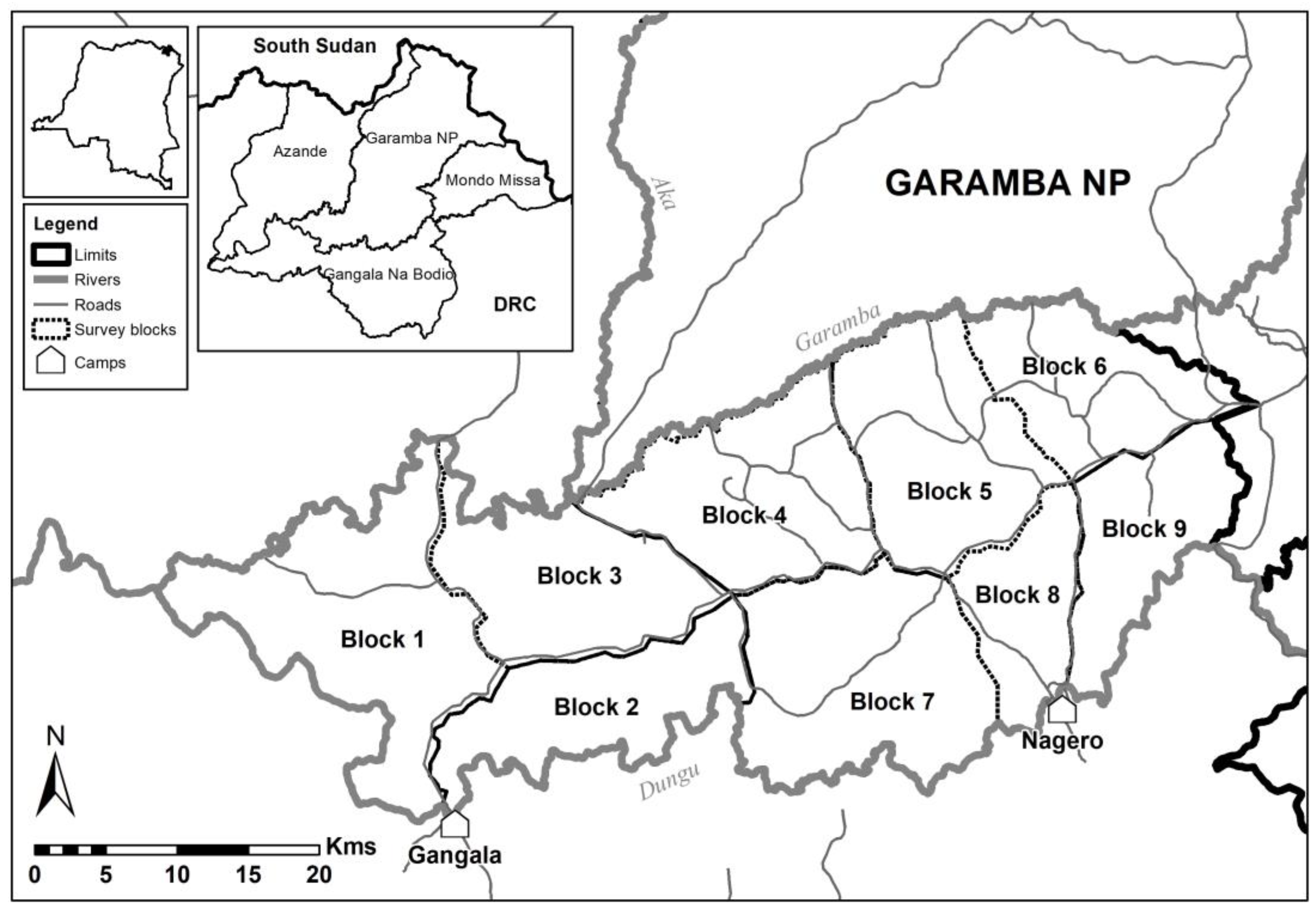
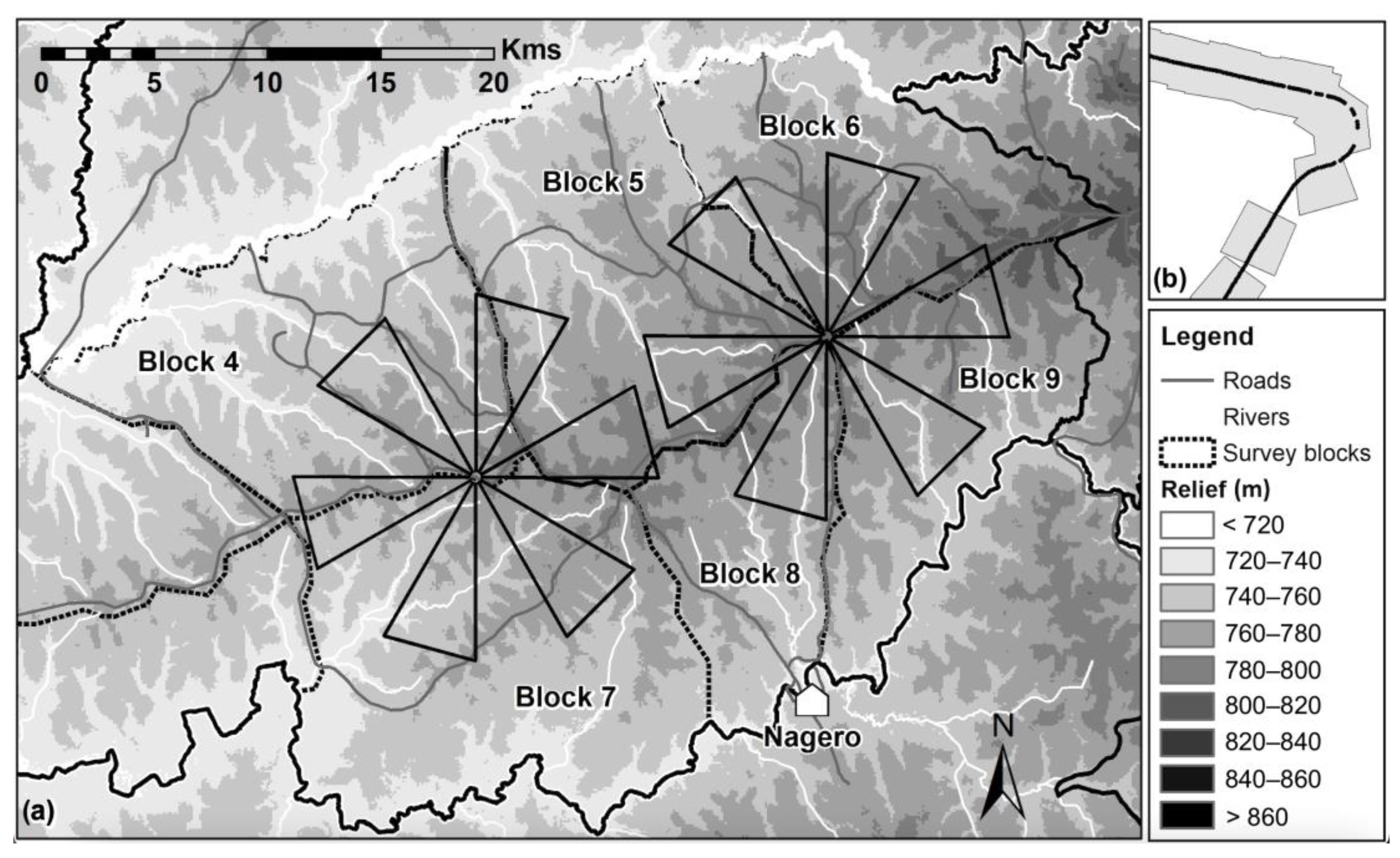
2.1. Study Area

Garamba National Park (hereinafter GNP) is located in North-Eastern Democratic Republic of Congo (hereinafter DRC), at the border with South Sudan (3°45′–4°41′ N. 28°48′–30°00′ E) and covers more than 5100 km2 (Figure 1). GNP is located in the Soudan-Guinean savannah biome. The park is predominantly grassland savannah with scattered trees dissected by riverine and small swamp forests, with mixed woodlands further north. The climate is tropical semi-humid with a short dry season observed between December and February [42,43].
GNP, a UNESCO World Heritage since 1981, is home for some of the last emblematic and endangered species in DRC, such as a unique hybrid form of elephants (Loxodonta cyclotis x africana), the endemic subspecies of Congolese giraffe (Giraffa camelopardalis congoensis), and the now already extinct northern white rhino (Ceratotherium simum cottoni) [42,44]. From the ’70 the park suffered increasing poaching pressure aggravated by armed conflicts in the area that caused animal populations drop to a critical level. Subsequently, the tests took place in the Southern part of the park where security permitted it and wildlife is found in greater densities. This section of the park is delimited by two of the main rivers, the Dungu and the Garamba. We worked only in the six Eastern management blocks, representing a total surface of 967.75 km2, as it was essential to limit movements within the park (blocks 4 to 9 in Figure 1).

2.2. Unmanned Aerial System

We used a small (6 kg with a 2.5 m wingspan) electrically powered fixed-wing UAS to collect the images. The UAS endurance was about 1 h for an average cruise speed of 14 m·s−1, representing ca. 40 km of safe equivalent linear data acquisition per flight survey. The small UAS was equipped with the APM open-source autopilot (http://firmware.eu.ardupilot.org, accessed on 15 January 2014) and programmed to follow a flight plan and take photos automatically through GPS positions. Control and flight plans were performed through the open-source software Mission Planner [http://firmware.eu.ardupilot.org, version 1.2.92 accessed on 15 January 2014] installed on the ground control station (GCS). Data transmission range through digital radio link (2.4 GHz) for live video transmission with a directional antenna was around 10 km in an open area with no physical obstacles.
The UAS was equipped with a Sony Nex7 digital still camera (6000 × 4000 pixels) mounted with a 16mm lens (sensor size 23.4 × 15.6 mm) producing true colors images, and two small video cameras for live retransmission for situation during flight operations. The payload was not mounted on a gimbal and all flight and orientation data were stored in the log file generated by the autopilot device that can be downloaded post-flight through the Mission Planner software.

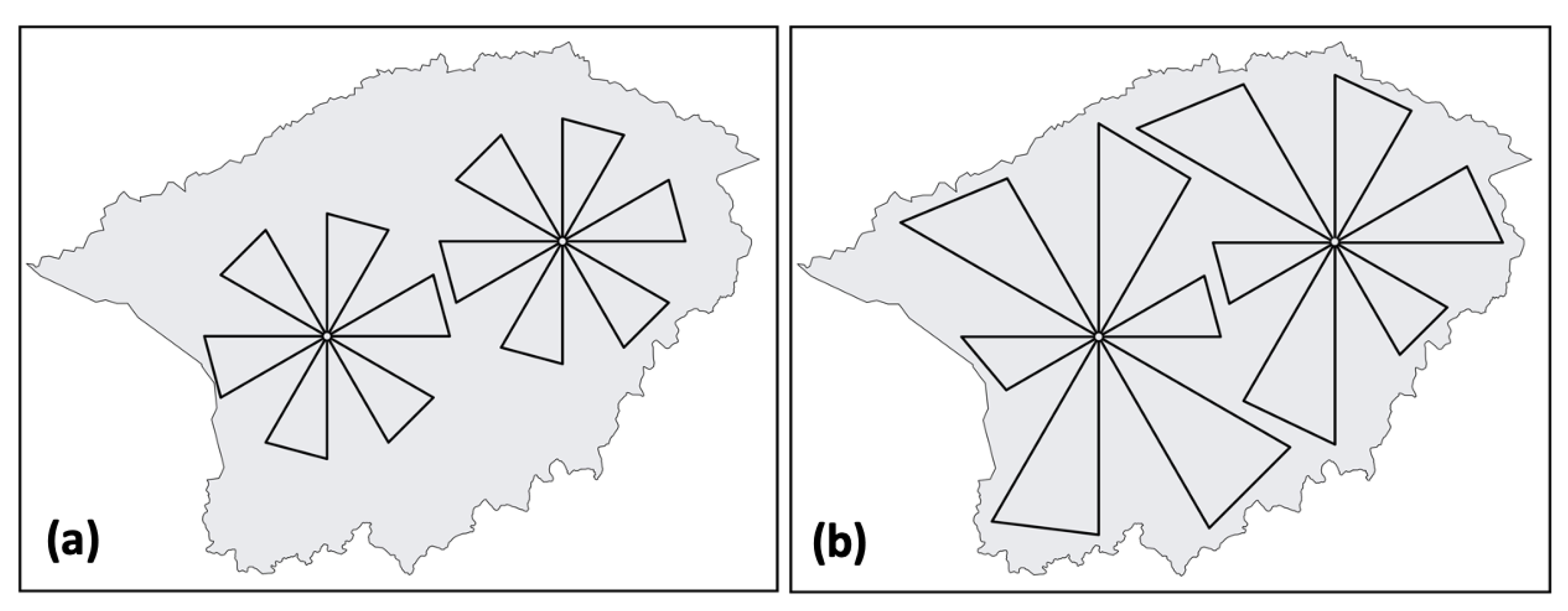
2.3. Flight Plan Design

With endurance and range being the main constraints, finding suitable take-off and landing sites is challenging. Good access routes are rare among a low-density road network in GNP, and off-road movements limited by the difficulties of the terrain and security issues. To maximize efficiency, several flights per day can be realized from a unique take-off site. Permanent control over the drone was also needed to be able to recover it swiftly in case of accident. In this context, we created a rosette pattern flight plan centered on the take-off/landing site (Figure 2). It allows the UAS to fly to its maximal range in every direction with almost the entire flight plan contributing to survey data, and offers the possibility of adapting the method to various contexts for large-scale game counts. Rosette shapes are easy to create and implement in the field as they only require defining a few waypoints in the flight plan. Each UAS survey could cover a length of 40 km of effective strips (excluding climbing and landing), and three flights per day could generally be done safely. This includes the time used to travel to and from the site, set-up the material, and data transfer, in Central African weather conditions where afternoon storms are very regular. We therefore proposed a pattern of 6 “petals” systematically separated by 30° angles, fitting within the maximal range of 10 km and which could be surveyed in a single day. Each petal consists in a triangle of 20 km of perimeter (8:4:8 km). Two opposing petals are covered during one flight of 40 km, for a total of 120 km per rosette (Figure 2a). The Southern part of the park is conveniently cut in half by one main road following the crest line from East to West, providing good radio communication conditions. We identified all the suitable spots along the road to set up the GCS and take-off sites. Only two full rosettes could fit in the 6 blocks survey area and we spread them as evenly as possible over the survey area (Figure 2a).

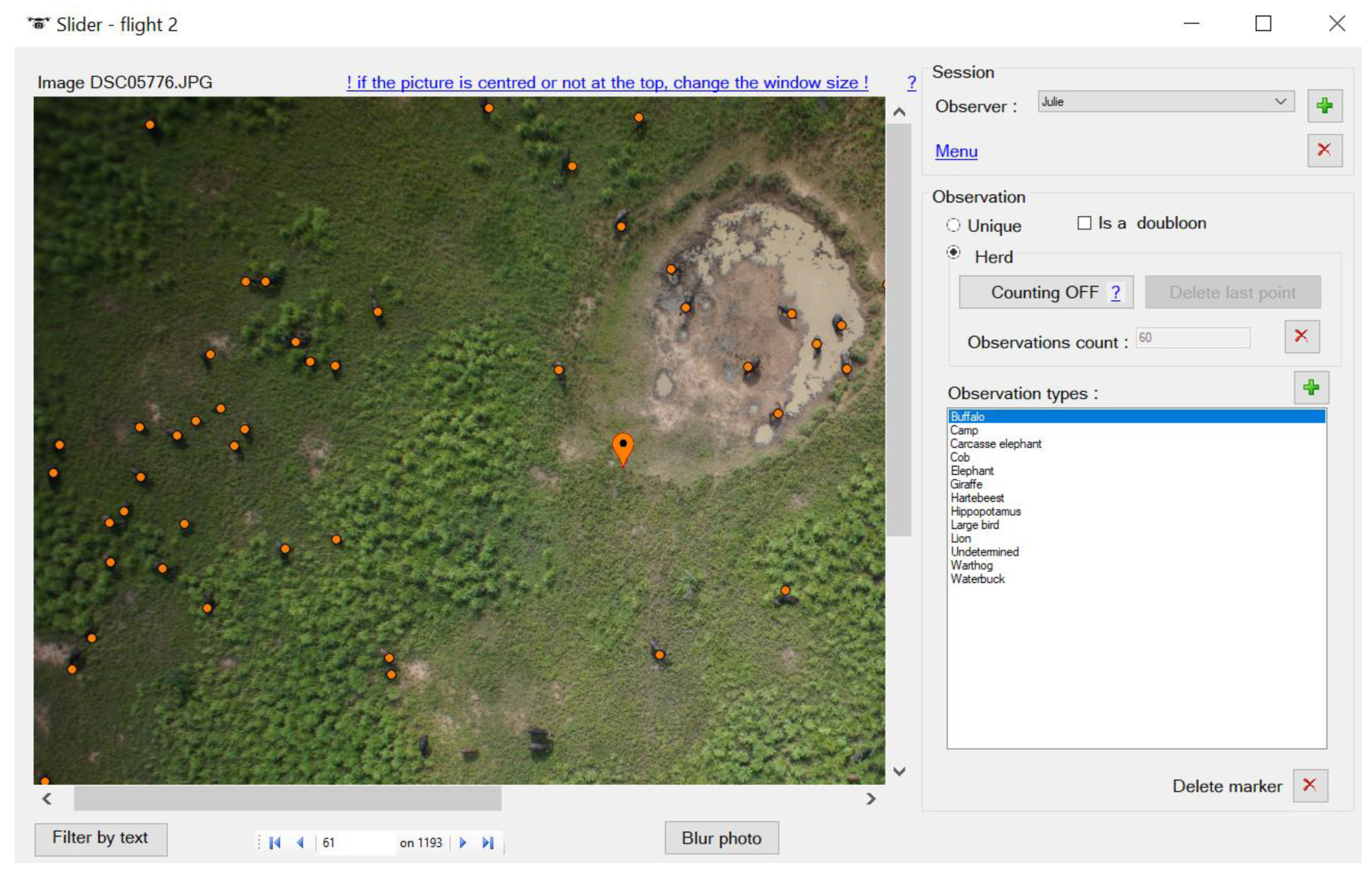
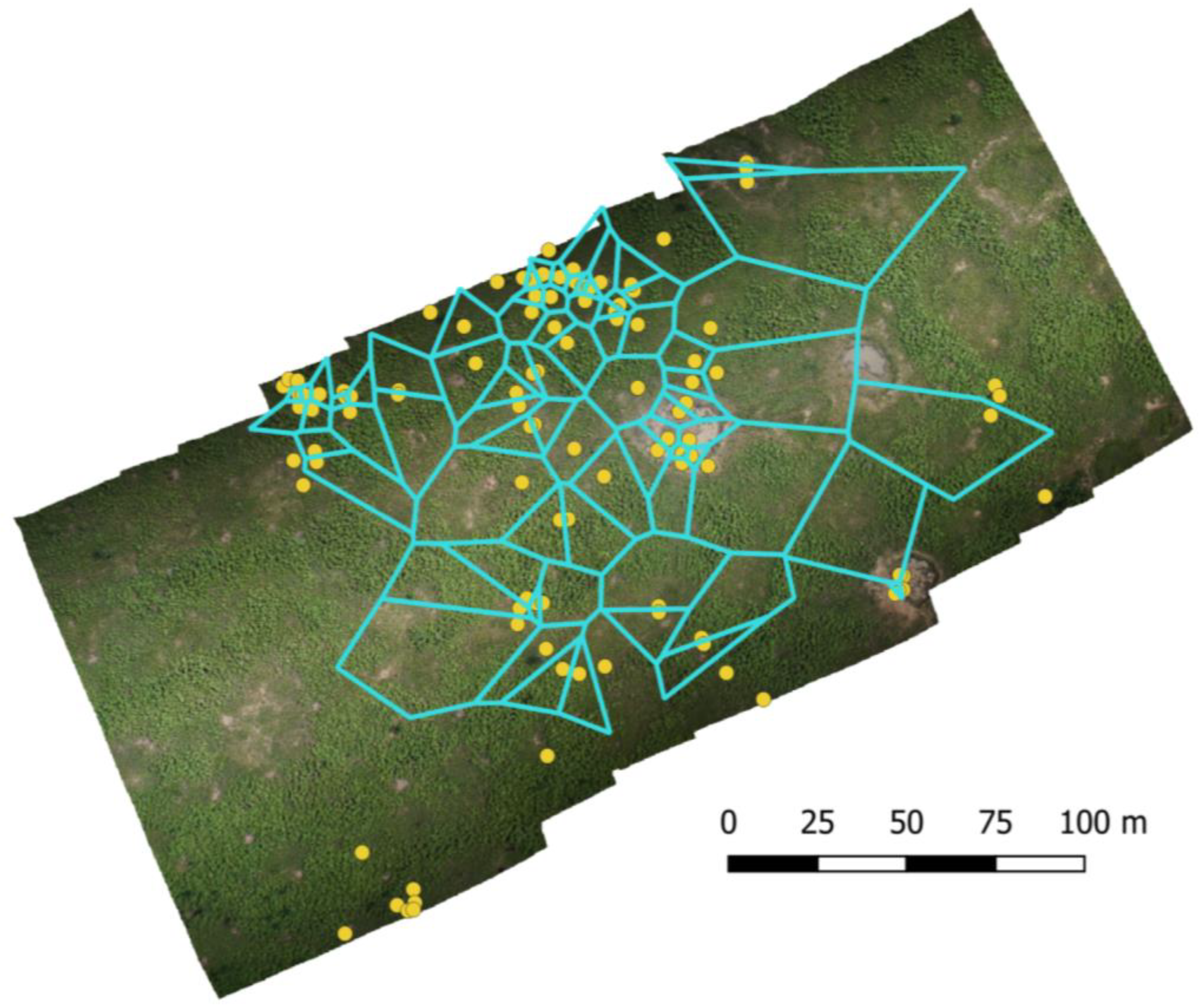
2.4. UAS Data Collection and Image Processing

We put our design and its efficiency to the test in real life conditions in the field in GNP to evaluate the logistical efforts and human resources costs of such survey. Six flights were performed in two half days in order to complete the two-rosette flight plan, doing one rosette per morning. We collected data over 2 seasons. We acquired a first dataset at the end of September 2014 in the late rainy season, when the grass is already high and animals are generally more dispersed. We performed a second flight plan in May 2015 at the beginning of the rains, when animals are still grouped and the grass cover is less dense. The UAS was set to fly at an average altitude between 90 and 100 m AGL as it was previously assessed a good compromise between detection for large- and medium-sized animals and covered bandwidth, given a ground sampling distance (GSD) of 2.5 cm/pixel [45]. The autopilot was programmed to take photos with enough longitudinal overlap to prevent gaps in the sampling strips. The general parameters of the performed flights and camera settings are recorded in Appendix A. All photos were geo-referenced using Mission Planner to match GPS position and orientation data of the UAV. To avoid oversampling at the center of the rosettes where lines of flight and the sampling strips overlap, we eliminated photos that were acquired within a radius of 250 m from the design center point. Moreover, it also removes the potential disturbance effect caused by the team arrival on site. Images from the take-off and landing phases were also discarded to keep only images that would then be reviewed for animal detection.
Two observers counted wildlife manually using the free software WiMUAS (http://www.gembloux.ulg.ac.be/gf/outilslogiciels/VolDrone2016.7z, accessed on 10 July 2016) created specifically for the purpose of annotating objects and estimating surfaces covered by drone images [45]. Appendix B shows an example of an annotated image. Observers’ results were merged to produce the most accurate count possible and correct species misidentifications. We identified giraffes, buffaloes (Syncerus caffer), hippopotamuses (Hippopotamus amphibius), hartebeests (Alcelaphus buselaphus), waterbucks (Kobus ellipsiprymnus), Ugandese kobs (Kobus kob) and warthogs (Phacochoerus africanus), all of which are counted in traditional manned aerial surveys.
We then evaluated the sampling strip surfaces by using the projected image footprints (Figure 2b) using a correction of the relief with SRTM data (1-Arc-Seconde, USGS). Animal densities were then estimated for both surveys. However, counts were mostly recorded for testing and time evaluation purpose, as reference densities were not available for comparison.

2.5. Simulations and Comparison with the Traditional Transect Method

In order to evaluate the statistical performance of our experimental method, we used theoretical simulations based on randomly generated animal population distributions to compare results obtained for both rosette and the classic transect flight plans.
We focused our analysis on two main well-represented animal categories in the park: medium to large size antelopes, and buffaloes. In GNP, these two groups show contrasting characteristics susceptible to influence the results of UAS counts. Indeed, buffaloes are a very aggregative species tending to stand very closely to each other in large groups of up to 400 individuals. This affects their distribution within the survey areas and generates great sample errors when estimating population densities, as sometimes large dense herds will be entirely missed and numbers strongly underestimated, or at the contrary if several transects pass through them, leading to overestimations [46]. Antelopes tend to be present in numerous smaller groups distributed more uniformly over the entire area and therefore the impact of the aforementioned issue is more limited.
The different steps used for both processes and algorithms generating population estimates are summarized in Figure 3 and detailed in the following sub-sections. All analyses were done using the software R [47]. The code can be found in Supplementary Material Code S1.

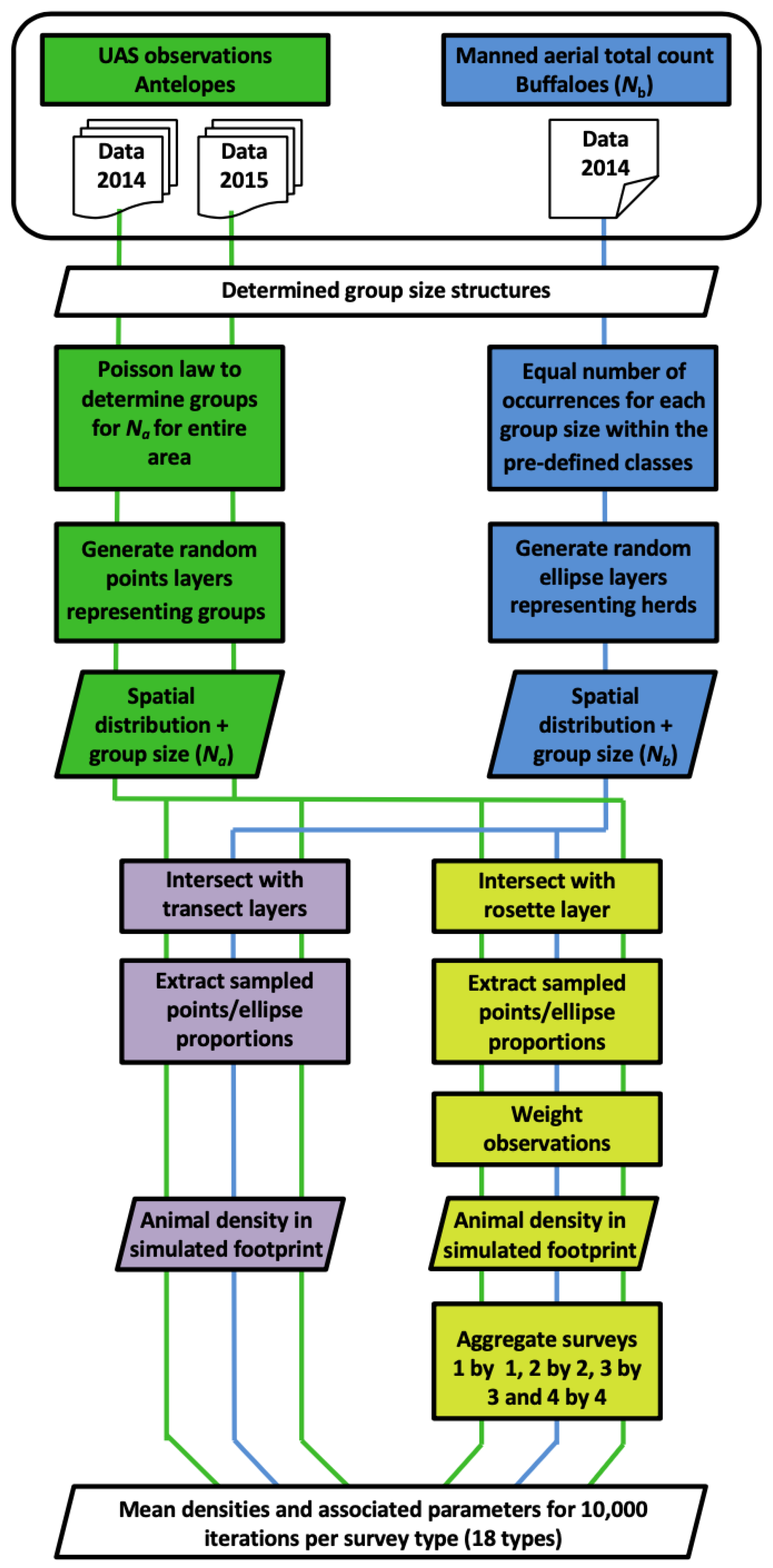
2.5.1. Animal Population Structures and Distribution Layers

Density and group structure for both antelopes and buffaloes had to be determined from previously acquired population data to create the most accurate base datasets for simulations.
For antelopes, spatial repartition and group structures could be derived from the observations from our UAS test counts, for both seasons separately as seasonal conditions would have an impact on their gregariousness due to water availability (respectively 2014 and 2015 datasets). We chose to merge data from the three main species together (kobs, waterbucks and hartebeests), as individual numbers were low, and the species were considered having similar behavior and repartition in regards with the needs of the study. Global antelope density for GNP was obtained by calculating the mean of the two UAS surveys of 2014 and 2015, and the estimated number of ungulates (Na) for the entire survey area is extrapolated from that value. Antelopes of the same species present on the same drone image or in a series of overlapping photos were considered as part of the same group. Theoretical group structures for Na ungulates were then generated with Poisson distributions as they could be considered randomly dispersed, for both seasons separately. The Poisson distribution is a single parameter special case of the negative binomial distribution, which, along with the truncated power-law distribution, is often used for animal group-size distribution modelization [48,49]. The size of the last group was automatically truncated to respect the total population size of Na animals. The animal groups were then randomly distributed within the study area. Each group was generated as a point associated to a group size value.
Buffaloes were not represented enough in the 2014 and 2015 observations based on UAS surveys to allow similar processing. Density and group structure were therefore derived from the manned aerial total count realized in the 2014 dry season by the park management team [50]. Recorded herd sizes were represented by classes of size and not absolute numbers. We considered the distribution of herd absolute sizes within each class as uniform. Therefore, we distributed the number of herds within each class equally among absolute group sizes to generate the theoretical population structure. The size of the last group was truncated to respect total population size Nb. As for antelopes, group centers were randomly distributed within the study area. To account for the spread of large herds in the case of buffaloes, groups were assimilated to ellipses (a = 2xb) randomly rotated. The mean surface by animal within a herd was extracted from an orthomosaic generated from the UAS images (see Appendix C for further explanations). The elliptic area covered by a group was then computed by multiplying the group size by the mean surface by animal. Full population distributions for both antelopes and buffaloes were generated for each iteration of the simulation.

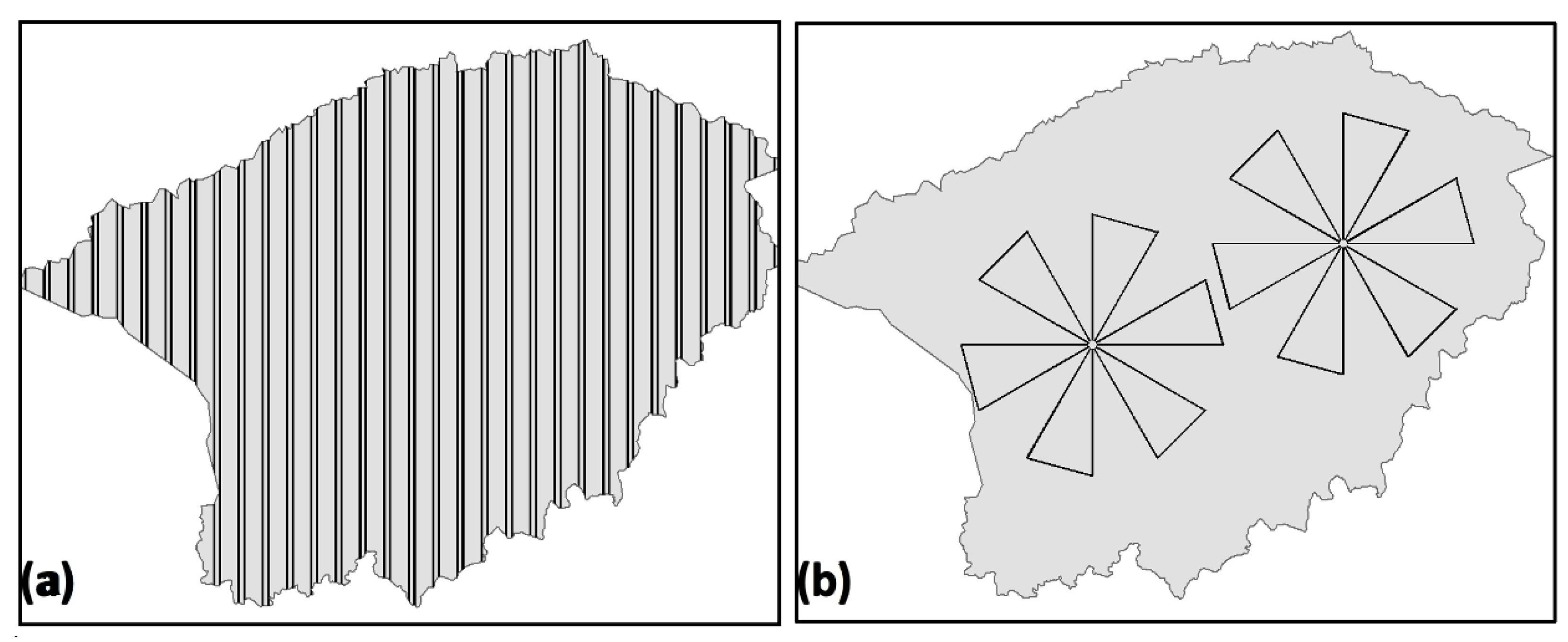
2.5.2. Simulated Sample Counts

For each survey, the spatial layers of antelope and buffalo groups were overlaid by the theoretical sampling strips provided by rosette and regular transect flight plans. The rosette sampling strips were based on the same rosette flight plan used to collect UAS data in the field and the strip width considered is an ideal buffer of 60 m from each side of the flight line, based on the footprint of photos regularly taken with the 16 mm pancake lens at an average 100 m flight height. Sampling strips for a traditional transect survey with manned aircraft at the target sampling effort (i.e., percentage of the study area surveyed) of 20% can be generated from lines of flight distant from 1.5 km and two observers each surveying a ground strip of 150 m on their respective side of the plane. Figure 4 shows the two flight plans and associated sampling strips footprints over the 6 survey blocks: the theoretical rosette flight plan represents a surveyed area of 28.53 km2 (2.38 km2 per petal), while the transect flight plan represents a surveyed area of 193.94 km2. Considering the extent of the management blocks surveyed (967.75 km2), the transect flight plan represents a 20.04% sampling rate, while the sampling rate of the rosette flight plan is 2.95%.
The number of antelopes counted during a survey was estimated by selecting the points located within the sampling strips and adding their associated group size values. A similar approach was used for buffaloes. The number of animals counted for each herd was derived from the proportion of the ellipse intersected by the sample strips. Because the rosette pattern is not evenly distributed over the area, under- and over-sampling may occur. To counter this issue, we applied a radial weighting of the observations relative to their position from the center of the rosette (see Appendix D). Animal density was then estimated for the animal group distribution layers for both seasons (2014 and 2015) for antelopes, and for buffaloes (2014). We generated 10,000 random iterations of each of the 3 types of animal distribution layers with the algorithm and overlapped them with both simulated flight plans.
We then wanted to evaluate the potential decrease in variability if the rosette flight plan was repeated several times and aggregated in order to increase the sampling rate, as repeatable flight plans are an advantage of UASs. We aggregated iterations of generated rosette counts by groups of 2, 3 and 4 for a total of again 10,000 iterations for each survey category. As 4 repetitions amounted to a sampling rate of 11.68%, we also added a new systematic transect flight plan of half the sampling rate (10.11%) for comparison of the efficiency. Transects in the new flight plan were therefore spaced out by 3 km. Ten thousands iterations were also processed.

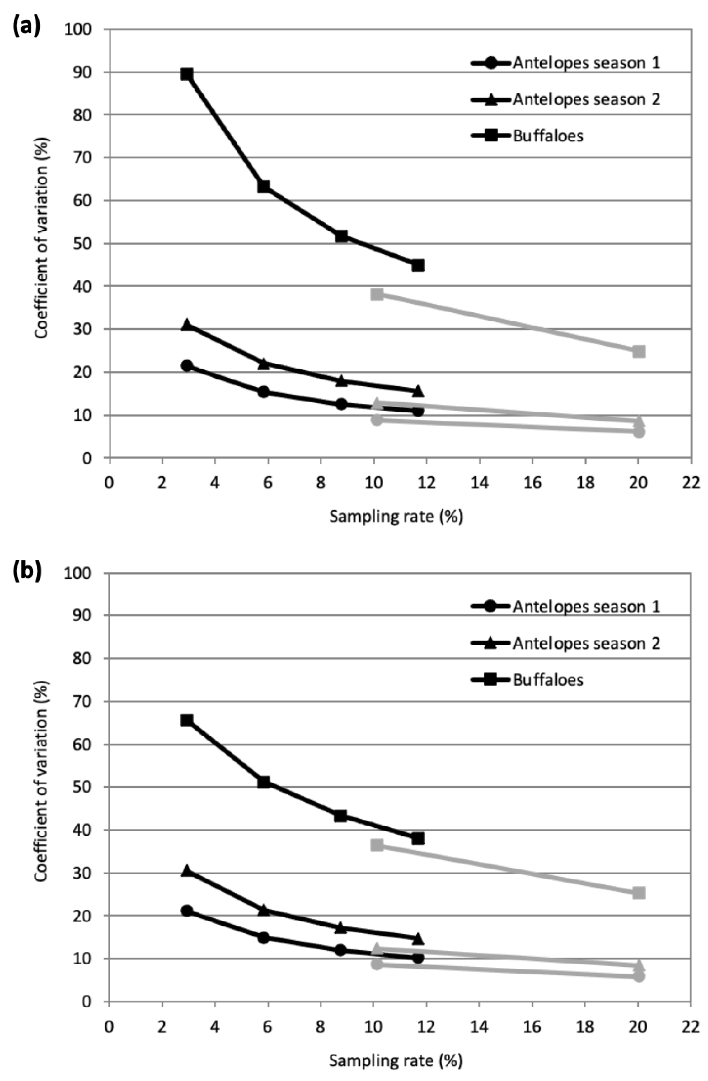
2.5.3. Performance of the Flight Plans

Mean density for each type of survey was estimated from the 10,000 respective iterations, as well as associated statistical parameters, such as mean error and coefficient of variation. Bias from the real density was also calculated, and equality between the real and estimated densities was tested with a Student t-test.
As animal density estimates are commonly calculated with the Jolly 2 method for classic transect counts (for statistic description see Jolly [39]), we also applied this method to our simulated counts for both transect and rosette flight plans, considering each petal as a sample unit.

3. Results

3.1. UAS Data Collection and Image Processing

Field experience showed that setting up the material for the first time takes 20 min, downloading the data and packing up after a flight takes another 20 min, while downloading the data and re-launching from the same spot takes half an hour. Three flights from the same take-off and landing site then took an average of 1 h 40 min in preparation on the ground.
The total number of images reviewed for animal identification with WiMUAS was 4654 for the 2014 survey and 7034 for the 2015 survey (details in Appendix A). It took approximately one hour per observer to review 500 images. The projected sampled areas obtained through WiMUAS were 24.50 km2 for 2014 and 33.44 km2 for 2015, representing respectively a sampling rate of 2.53% and 3.46%. Variation in estimated surface covered would normally vary, as orientation of the UAS will always be imprecise. However, the significant difference of sampling rate despite following the same flight plan is probably due to automatic triggering dysfunctions, as large gaps of missing photos could be found along the flight lines.
The complete results of the UAS counts and associated statistical parameters can be found in Appendix E, albeit most species were in too low number to provide valuable information. In 2014 antelope density was estimated at 2.33 individuals/km2, and at 4.25 in 2015.

3.2. Simulations and Comparison with the Traditional Transect Method

3.2.1. Population Structures and Distribution Layers

In 2014, only 57 antelopes were counted, distributed in 31 groups, for an average group size of 1.84. In 2015, 142 antelopes were found, distributed in 30 groups with an average group size of 4.71 (see Appendix F). One group of 36 kobs made up for almost a quarter of the animals detected during the latter survey. The mean density of antelopes for both seasons is 3.29 n/km2 and gives an estimated mean total population Na = 3180 antelopes for the six survey blocks. We then generated random distribution layers with the Poisson algorithms for 2014 and 2015, of respectively 1589 and 671 points.
Buffaloes had a population density of 4.98 n/km2 for the 6 blocks of the 2014 total count. Layers of 234 randomly distributed ellipses representing the number of herds were generated. The mean surface occupied by an animal in the herd was calculated at 118 m2, determining the ellipse sizes according to the group size structure.

3.2.2. Simulated Sample Counts and Performance

Table 1 shows the resulting antelope densities for 10,000 iterations of each simulated survey type (transect flight plans at 1.5 and 3 km, and 1 to 4 repetitions of the rosette flight plan, respectively) with their statistical parameters. Table 2 shows the same results for buffaloes.
For antelopes, the resulting mean densities after 10,000 iterations for each type of survey do not differ significantly from the theoretical density derived from UAS surveys, all bias being very low (all under 0.38%). Equally, for buffaloes, all the estimated densities do not differ significantly from the expected density obtained from the manned aerial total count. Coefficients of variation (CV) are good estimators of the stability and efficiency of the methods as they indicate the volatility expected for the population density estimates. Our results show a very strong heterogeneity when only one repetition of the rosette flight plan is done. The CV then reduces quickly with each repetition of the rosette flight plan for both antelopes and buffaloes (Figure 5a). In the case of antelope density estimates, the CV curves tend to flatten quickly. After four repetitions, it tends to align with this of transect surveys following the increase in sampling rate, although it remains slightly higher.
Four repetitions of the rosette flight plan produced density with CVs that remain close to 15% for both seasons; almost double as can be expected with a classic systematic transect sampling count. Comparison from both antelope population structures shows the CV is lower for antelopes during season 2014 where group sizes are smaller. It increases for season 2015 where group structure is more aggregative and larger groups are recorded, highlighting the impact of gregariousness of the species on density estimation.
Results for buffaloes are consistent with these trends, with CVs observed that are much higher than for antelopes, as expected for a highly aggregative species. Doing no repetition of the rosette survey has a strong potential to lead to excessively high numbers, but can also miss out on most or even all animals and severely underestimate the density (Table 2). Figure 5a shows the CV curve drops steeply after repeating twice the rosette flight plan, however it flattens at a slower rate than for antelopes, staying at high numbers even for the classic transect sampling flight plan. Surprisingly, four repetitions of the rosette flight plan still produce a higher CV than an equal sampling rate transect survey in every case, and the rosette curves flatten above the transect curves. Estimates performed with the Jolly 2 method presents similar CV curves, except for rosace estimates of buffaloes which tend to perform better (Figure 5b).
The ratio between the CVs associated with the density estimates obtained from 10,000 iterations for each simulated survey type and CVs calculated with the Jolly 2 method shows consistent results for antelope populations (Figure 6). However, the Joly 2 method shows a reduced variability in the case of buffalo density estimates with all repetitions of the rosette flight plan, up to 25% less with just one repetition.

4. Discussion

4.1. Rosette Flight Plan

Transects have been widely used for aerial sampling counts as they allow the aircraft to operate at maximum efficiency, making the proportion of “dead time” between pairs low for a plane [1,46]. However, what was an advantage for manned planes is still an issue with small UAS, which are limited in range and flight time, and where time took turning between transects and going back and forth the landing spot is a significantly higher percentage of the shorter flight time. Fortunately, UAS offer possibilities for more complex flight plans, as their autonomous navigation system is more flexible and not impacted by flying fatigue [7]. The rosette flight plan addresses the specific challenges of suitable operations sites, circular communication range, and ground team movement efficiency. While comparison of path length with transects is not directly possible due to difference in strip width, during transect counts 20 to 30% of the path is not exploited (back and forth from landing strip and all turns between transects), while with rosettes, 98% of flight lines are exploited. Comparatively to other various potential designs such as spirals, or concentric circles e.g., they also require less waypoints to prepare the flight plan. However, our design presents some limitations compared to systematic transects. Transects cover systematically the entire survey area, and are flown from a baseline generally following main environmental gradients, such as rivers (Figure 1 and Figure 4). Rosettes were placed according to the ground and range limitations, and as a result don’t cover equally the different habitats. In this case, they don’t sample the main rivers making the Northern and Southern limits of the survey area, potentially leaving out important habitats and observations. Indeed, our assumption was that animals were spread evenly across the park, as water and green grass were both available everywhere during the survey seasons. But our 2015 antelope survey is closer to the dry season, and it can already have a noticeable influence on the distribution. To prevent such issue in the future, we can easily imagine variations of the design, such as presented in Figure 7, with “petals” of different length to cover more evenly the study area, or with more petals per rosette to increase sampling. Our design was specifically adapted to our material constraints and shows the possibility of a new functional method, although not limited to it, as UAS are developing and getting longer range.

4.2. Simulated Survey Results

As seen in Figure 4 and Figure 7, the rosette flight plan designed to fit our small UAV covers a much smaller sampling rate (2.95%) than traditional transects recommended for African ungulates surveys [46]. To overcome this limitation, we aggregated four repetitions of the rosettes, and achieved a sampling rate of 11.80% (114.19 km2) compared to 20.04% (193.94 km2) with traditional systematic transects. Indeed, the CVs for the aggregated rosette surveys decreases much faster than the sampling area covered increases, following an asymptotic curve. Interestingly, the rosette CV curves do not align completely with these of transect survey modalities. For an equal sampling rate, the CVs obtained with the rosette sampling method remain higher. This could be explained by the ponderation factor applied to observations in the rosettes, which creates some noise in the data by giving more weight to observations at the extremities.
A coefficient of variation under 10–15% is often used as rule-of-thumb for accurate herbivore density estimates [51] and would be acceptable for most antelope counts. Our four aggregated rosette flight plans only produced estimates with a CV around 15% for antelope populations. While a traditional transect flight plan undoubtedly improves results, the increased precision might not necessarily always be required to fulfill management goals. Equally, a fifth repetition would be enough to drop under 10% and make the design completely relevant. Moreover, the transect simulations display perfect theoretical results. However, during aerial surveys in the field, the counts are subject to observer’s bias who can miss animals and tend to underestimate densities. The bandwidth within which observers are counting is also imprecise, based on average flight height and approximate projection of the footprint between the streamers. Orientation and flight data collected by the drone autopilot allow for a more precise projection of the image footprints and more accurate density estimates.
In the case of buffaloes, our models showed the significant impact of gregariousness on density estimate accuracy and precision, as expected. As the CV curve does not flatten as quickly as for antelopes, the impact of the reduced sampling rate of the rosette flight plan is much bigger, with coefficient of variation reaching over 40% with four repetitions. We would therefore not recommend using the rosette sampling design for highly aggregative species (buffaloes, elephants, hippos, …), as it will potentially miss important information on large herds size and structure. We advise to monitor them with more appropriate methods such as total counts [52], or combination of methods such as [53] proposed in their innovative survey combining drone flights with GPS collars fitted on some animals within large herds. More precise stratification of the survey areas based on previous knowledge could also be used, increasing the survey effort where it is more likely to yield higher results, such as it was done recently to census hippos [40].

4.3. Performance of the Rosette Flight Plan in the Field

The UAS surveys performed with the new rosette flight plan in September 2014 and in May 2015 were realized in order to field-test the feasibility of our design and its logistical practicalities, as well as gathering data on population structures in order to implement precise simulations. It does not have the vocation to be compared with the simulation results or the manned aerial census performed in the park. Field tests nonetheless allowed us to confirm that it is possible to identify and count the main species of medium-to-large mammals present in Garamba NP. Almost all the species recorded by the last aerial total count performed in GNP [50] were easily identified on the UAS images by the observers, such as hartebeests, kobs, waterbucks, buffaloes, giraffes and hippos. Detection differences between the two observers were sometimes important but were compensated at the end by the experienced observer. These findings are consistent with expectations that trained observers used to work on aerial counts in a particular environment will perform better [26]. In this particular case of drone census, experience with the different species visualization on near-nadir images provides a clear advantage to the observer and should therefore be part of the training of new observers. The elephants were notably absent from our UAS surveys despite being the flagship species of the park and the main focus of aerial censuses conducted in the area. Although surprising, the complete absence of elephants on the images highlights the difficulty of estimating wide-ranging aggregative species populations. As the groups tend to move together to follow resource availability and can cover very long distances, they can be missed entirely. The same situation relates to the variations in buffalo density estimations.
If we consider an aggregation of four to five repetitions satisfying in terms of population estimates with the rosette flight plan, we can evaluate logistics compared to manned aerial surveys. Indeed, four repetitions of our rosette flight plan would likely take 4 days of work in the field with currently available UAS models, while a manned plane could cover the 644 km of transects in less than 2 days. In terms of pure man-hours, this analysis disfavors UAS surveys. Ref. [54] had similar negative cost comparison for East and Southern Africa. However, these approximative costs don’t relate well to operation costs experienced in countries of Central and West Africa, where getting planes, fuel and pilots on site can be a matter of days and exponentially expensive. When many parks and protected areas do not have the budget to support a dedicated plane and pilot on site full time, and contracting with external providers proves challenging, UAS can be a cheap alternative. From our experience, we can assume that a permanent employee based in the park could be trained easily on a simple UAS, and take these responsibilities on top of his other duties at a reduced cost [7]. However, in case of large-scale surveys requiring up to 10 rosettes, the heavy requirements in terms of logistics and days in the field render the method largely inefficient until a technological leap happens. As cost/efficiency ratios of UAS keeps decreasing over time, several possibilities will become available [13,22,55]. It could be the use of multiple UAS [53,56], or even swarm of cheap UAS, covering multiple rosettes at the same time; or solar UAV (https://sunbirds.aero, accessed on 24 February 2021) capable of staying airborne several hours. Another interesting possibility is to have a camera on each side of the drone, doubling the bandwidth and sampling rate without increasing the logistics.
Finally, to generalize the use of such new methods, improving the processing of the huge volumes of images is the next important step [12,13,22]. We calculated an average of 9 h was necessary to review the data of one full rosette flight plan and annotate all animals manually. Five repetitions of the design would therefore take an observer 45 h of work. This is a fairly long processing time, and observer fatigue can reduce the accuracy of his detections. Equally, huge progress has been made in automatic detection and deep learning methods over the last five years, and it opens a very promising future for the technique [22,57,58]. It would likely be possible to develop rapidly semi-automatic detection algorithms to select automatically all the images with wildlife and ask for an observer to confirm observations manually [54,59,60].

5. Conclusions and Recommendations

The rosette flight plan proved particularly easy to create and implementation in the field was successful, making it an adequate method for teams with basic flight training. Despite its advantages, based on numerical simulations, the rosettes give less precise estimates than systematic transects at a given sampling rate. As with systematic transect sampling, the method was found to be giving higher coefficient of variation for highly aggregative species such as buffaloes and elephants. Therefore, we would recommend using this method, or an adaptation with various petal sizes, mostly for medium to large-size species that tend to disperse widely and more randomly in their environment.
To reach satisfying estimates for antelope populations, a fifth repetition could be enough. As only a few rosettes are needed to cover vast areas, logistics and movements can be limited, especially as the technology evolves towards better endurance and flight radius. This method would be particularly relevant in the case of remote protected areas lacking access to aircraft, especially as small UAV can be used for a variety of tasks such as various mapping objectives, surveillance, and specific wildlife surveys (rivers and ponds monitoring, wetlands surveying, etc.). Moreover, use of UAV for regular surveys limits the risk of human harm tremendously, especially in wild places where aerial accidents have dramatic consequences. This fulfills our first objective to design an innovative new flight plan and sampling protocol adapted to small UAS constraints. The next step following our study would be to implement a full-scale rosette survey with five repetitions conducted the same month as a classic aerial census in order to compare the theoretical results with real conditions.

Supplementary Materials

The following supporting information can be downloaded at: https://www.mdpi.com/article/10.3390/drones7030208/s1, Code S1: R code for the simulation process.

Author Contributions

Conceptualization, J.L., P.L. and C.V.; methodology, J.L and P.L.; software, J.L. and S.Q.; validation, P.L. and Y.B.; formal analysis, P.L. and J.L.; investigation, J.L.; resources, J.L.; data curation, J.L.; writing—original draft preparation, J.L.; writing—review and editing, J.L., P.L., C.V., Y.B., S.L. and A.M.; visualization, J.L.; supervision, P.L. and C.V.; project administration, P.L.; funding acquisition, P.L. All authors have read and agreed to the published version of the manuscript.

Funding

The research was funded under the Letter of Agreement with the Center for International Forestry Research [CIFOR] in the framework of the project Forests and Climate Change in the Congo [FCCC], funded by the European Union [EU] under Grant Number DCI-ENV/2012/309143.

Data Availability Statement

Data is contained within the article or Supplementary Materials.

Acknowledgments

The authors would like to thank the ICCN, African Parks Network and R&SD office for their support in the field, as well as all participating team members and other actors for their help. Special thanks go to Philippe Bouché, who passed away before the submission of this manuscript, but was instrumental in the success of this survey by his great knowledge of wildlife censuses and relevant advice, and his constant support.

Conflicts of Interest

The authors declare no conflict of interest. The funders had no role in the design of the study; in the collection, analyses, or interpretation of data; in the writing of the manuscript; or in the decision to publish the results.

Appendix A

Flight parameters are presented in Table A1.
Table A1. Parameters of the survey flights realized and images collected and reviewed for animals identification.
2014, Late Rainy Season2015, Early Rainy Season
Rosette 1Rosette 2Rosette 1Rosette 2
Flight Number R1F1R1F2R1F3R2F1R2F2R2F3R1F1R1F2R1F3R2F1R2F2* R2F3a* R2F3b
Flight Time (min)50454550455050555550455025
Conditions and camera parametersWeatherCloudy, wind 2–6 m/sCloudy, stormy, wind 3–6 m/sSunny to partially cloudy, wind 2–5 m/sSunny to partially cloudy, wind 2–5 m/s
ISO200400200200
Shutter speed1600200020002000
Trigger distance (m)12162525
PhotosTotal number7846225871300993108710481330131613721382981670
Discarded13690711308017983132869613837788
Blurry3231573458182055
Reviewed for animals 64553051311559069059611193122212581224599577
* During the last flight of survey 2 we discovered the camera stopped taking photos mid-flight due to a connection problem in the hardware. We re-launched the plane after repairs for a last flight covering only the last petal to finish the survey, hence second rosette flights 3a and 3b.

Appendix B

Example of an UAS images in WIMUAS viewer with annotated buffaloes is presented in Figure A1.
Figure A1. Buffaloes detected on the images pointed with WiMUAS. In case of groups or herds of the same species, multiple dots can be attached to one point and considered as a cluster.
Drones 07 00208 g0a1

Appendix C

Estimation of the animal density within the buffalo herds. A set of 10 successive images acquired during one of the 2014 rosettes covered partially a large herd of buffalos. These images were processed with the software Metashape (AgiSoft Metashape Standard (Version 1.6.5), 2020, retrieved from http://www.agisoft.com/downloads/installer/, accessed on 12 November 2020) in order to produce an orthoimage with a pixel size of 2.4 cm. Using this orthoimage as background, we digitized manually a layer of 105 points representing the position of every visible buffalo. The function voronoi (package dismo) was then used to generate a layer of Voronoï polygons for this set of points (Figure A2). All the polygons that were partially outside the orthoimage footprint were discarded. The median area of the 75 remaining polygons was considered as the mean surface occupied per animal inside the herd.
Figure A2. Orthoimage of the partial herd of buffaloes. Yellow dots each represent an individual buffalo. In blue are the generated Voronoï polygons.
Drones 07 00208 g0a2

Appendix D

Radial weighting. In the rosette design, the petals are made of two radial segments and one tangential segment (Figure A3).
Figure A3. Radial and tangential segments of the rosette design. For a di distance to the center of the rosette, 1/wi corresponds to the proportion of the corresponding circle (radius = di) that is sampled.
Drones 07 00208 g0a3
The radial segments are considered to have a variable sampling rate along the line. A weighting factor inversely proportional to the distance between the observations and the center of the rosette was used to compensate for this variation using the following Equations (A1)–(A4):
d = n w a r e a
n w = i = 1 m s i . w i w . m
w i = 2 . . d i 2 . n p . b w   for radial segments
w i 2   for tangential segments
where,
  • d: population density (animal/km2)
  • n w : weighted number of animals inside a rosette
  • area: area of the sample bands (km2)
  • m: number of groups of animals inside the sample bands
  • s i : number of animals of group I that are inside the sample bands
  • w i : weighting factor for group i
  • d i : distance between group I and the rosette center (m)
  • np: number of petals in the rosette
  • bw: width of the bands surveyed by the UAV (m).
  • w : mean weight considering an entire rosette.
  • w i : in the case of tangential segments, the weighting considers the fact that these segments represent approximately half the circumference of the circle in which the rosette is inserted.
  • w was computed by numerical integration using raster calculator tool in QGIS. The value of 14.32 has been obtained considering the petal configuration presented in this study.

Appendix E

Results of the UAS rosette animal counts in the field are presented in Table A2.
Table A2. Results of the rosette animal counts for both seasons. Data are presented for the main species recorded and all antelopes (kobs, waterbuck and hartebeests) have been merged in one category, as described in methodology.
Sampling Strip Area (km2)Nbr AntelopesNbr GiraffesNbr BuffaloesNbr WarthogsNBR Hippos
2014Rosette 112.3730/249923
Rosette 212.1327/102735
Total24.5057/2593658
Density (n/km2)2.33/10.571.472.37
Estimated total population2252/10,23114222291
Standard error (n/km2)136.41/13,210.421025.30702.14
CI 95% (n/km2)±189/±18,308±1421±973
(%)±8.40 /±178.96±99.93 ±42.48
2015Rosette 117.5050101331647
Rosette 215.9492047731
Total33.44142101802378
Density (n/km2)4.250.305.380.692.33
Estimated total population410928952096662257
Standard error (n/km2)1994.40391.033182.99325.14507.01
CI 95% (n/km2)±2764±542±4411±451±703
(%)±67.26 ±187.26 ±84.68 ±67.70 ±31.13

Appendix F

Repartition of group sizes for antelope and buffalo populations are presented in Figure A4.
Figure A4. (a) Group structure of antelope populations from UAS observations acquired in 2014 and 2015. (b) Group structure for buffaloes as reported in the 2014 manned aerial total count.
Drones 07 00208 g0a4

References

  1. Jachmann, H. Estimating Abundance of African Wildlife: An Aid to Adaptive Management; Kluwer Academic Publishers: Boston, MA, USA, 2001; ISBN 978-1-4615-1381-0. [Google Scholar]
  2. Jachmann, H. Evaluation of Four Survey Methods for Estimating Elephant Densities. Afr. J. Ecol. 1991, 29, 188–195. [Google Scholar] [CrossRef]
  3. Wang, D.; Shao, Q.; Yue, H. Surveying Wild Animals from Satellites, Manned Aircraft and Unmanned Aerial Systems (UASs): A Review. Remote Sens. 2019, 11, 1308. [Google Scholar] [CrossRef] [Green Version]
  4. Bouché, P.; Lejeune, P.; Vermeulen, C. How to Count Elephants in West African Savannahs? Synthesis and Comparison of Main Gamecount Methods. Biotechnol. Agron. Sociol. Environ. 2012, 16, 77–91. [Google Scholar]
  5. Dunham, K.M. Trends in Populations of Elephant and Other Large Herbivores in Gonarezhou National Park, Zimbabwe, as Revealed by Sample Aerial Surveys. Afr. J. Ecol. 2012, 50, 476–488. [Google Scholar] [CrossRef]
  6. Watts, A.C.; Perry, J.H.; Smith, S.E.; Burgess, M.A.; Wilkinson, B.E.; Szantoi, Z.; Ifju, P.G.; Percival, H.F. Small Unmanned Aircraft Systems for Low-Altitude Aerial Surveys. J. Wildl. Manag. 2010, 74, 1614–1619. [Google Scholar] [CrossRef]
  7. Christie, K.S.; Gilbert, S.L.; Brown, C.L.; Hatfield, M.; Hanson, L. Unmanned Aircraft Systems in Wildlife Research: Current and Future Applications of a Transformative Technology. Front. Ecol. Environ. 2016, 14, 241–251. [Google Scholar] [CrossRef]
  8. Sasse, D.B. Job-Related Mortality of Wildlife Workers in the United States, 1937–2000. Wildl. Soc. Bull. 2003, 31, 1015–1020. [Google Scholar]
  9. Mulero-Pázmány, M.; Stolper, R.; van Essen, L.D.; Negro, J.J.; Sassen, T. Remotely Piloted Aircraft Systems as a Rhinoceros Anti-Poaching Tool in Africa. PLoS ONE 2014, 9, e83873. [Google Scholar] [CrossRef] [PubMed] [Green Version]
  10. Johnston, D.W. Unoccupied Aircraft Systems in Marine Science and Conservation. Annu. Rev. Mar. Sci. 2019, 11, 439–463. [Google Scholar] [CrossRef] [Green Version]
  11. Chabot, D.; Bird, D.M. Wildlife Research and Management Methods in the 21st Century: Where Do Unmanned Aircraft Fit In? J. Unmanned Veh. Syst. 2015, 3, 137–155. [Google Scholar] [CrossRef] [Green Version]
  12. Linchant, J.; Lisein, J.; Ngabinzeke, J.S.; Lejeune, P.; Vermeulen, C. Are Unmanned Aircraft Systems (UASs) the Future of Wildlife Monitoring? A Review of Accomplishments and Challenges. Mammal Rev. 2015, 45, 239–252. [Google Scholar] [CrossRef]
  13. López, J.J.; Mulero-Pázmány, M. Drones for Conservation in Protected Areas: Present and Future. Drones 2019, 3, 10. [Google Scholar] [CrossRef] [Green Version]
  14. Hodgson, A.; Kelly, N.; Peel, D. Unmanned Aerial Vehicles (UAVs) for Surveying Marine Fauna: A Dugong Case Study. PLoS ONE 2013, 8, e79556. [Google Scholar] [CrossRef] [Green Version]
  15. Michez, A.; Broset, S.; Lejeune, P. Ears in the Sky: Potential of Drones for the Bioacoustic Monitoring of Birds and Bats. Drones 2021, 5, 9. [Google Scholar] [CrossRef]
  16. Kloepper, L.N.; Kinniry, M. Recording Animal Vocalizations from a UAV: Bat Echolocation during Roost Re-Entry. Sci. Rep. 2018, 8, 7779. [Google Scholar] [CrossRef] [Green Version]
  17. Desrochers, A.; Tremblay, J.A.; Aubry, Y.; Chabot, D.; Pace, P.; Bird, D.M. Estimating Wildlife Tag Location Errors from a VHF Receiver Mounted on a Drone. Drones 2018, 2, 44. [Google Scholar] [CrossRef] [Green Version]
  18. Hodgson, J.C.; Mott, R.; Baylis, S.M.; Pham, T.T.; Wotherspoon, S.; Kilpatrick, A.D.; Segaran, R.R.; Reid, I.; Terauds, A.; Koh, L.P. Drones Count Wildlife More Accurately and Precisely than Humans. Methods Ecol. Evol. 2018, 9, 1160–1167. [Google Scholar] [CrossRef] [Green Version]
  19. Rees, A.F.; Avens, L.; Ballorain, K.; Bevan, E.; Broderick, A.C.; Carthy, R.R.; Christianen, M.J.A.; Duclos, G.; Heithaus, M.R.; Johnston, D.W.; et al. The Potential of Unmanned Aerial Systems for Sea Turtle Research and Conservation: A Review and Future Directions. Endanger. Species Res. 2018, 35, 81–100. [Google Scholar] [CrossRef] [Green Version]
  20. Morley, C.G.; Broadley, J.; Hartley, R.; Herries, D.; McMorran, D.; McLean, I.G. The Potential of Using Unmanned Aerial Vehicles (UAV) for Precision Pest Control of Possums (Trichosurus Vulpeca). Rethink. Ecol. 2017, 2, 27–39. [Google Scholar] [CrossRef]
  21. van Andel, A.C.; Wich, S.A.; Boesch, C.; Koh, L.P.; Robbins, M.M.; Kelly, J.; Kuehl, H.S. Locating Chimpanzee Nests and Identifying Fruiting Trees with an Unmanned Aerial Vehicle. Am. J. Primatol. 2015, 77, 1122–1134. [Google Scholar] [CrossRef] [PubMed]
  22. Fust, P.; Loos, J. Development Perspectives for the Application of Autonomous, Unmanned Aerial Systems (UASs) in Wildlife Conservation. Biol. Conserv. 2019, 241, 108380. [Google Scholar] [CrossRef]
  23. Butcher, P.A.; Colefax, A.P.; Gorkin, R.A., III; Kajiura, S.M.; López, N.A.; Mourier, J.; Purcell, C.R.; Skomal, G.B.; Tucker, J.P.; Walsh, A.J.; et al. The Drone Revolution of Shark Science: A Review. Drones 2021, 5, 8. [Google Scholar] [CrossRef]
  24. Inman, V.L.; Kingsford, R.T.; Chase, M.J.; Leggett, K.E.A. Drone-Based Effective Counting and Ageing of Hippopotamus (Hippopotamus Amphibius) in the Okavango Delta in Botswana. PLoS ONE 2019, 14, e0219652. [Google Scholar] [CrossRef] [Green Version]
  25. Gooday, O.J.; Key, N.; Goldstien, S.; Zawar-Reza, P. An Assessment of Thermal-Image Acquisition with an Unmanned Aerial Vehicle (UAV) for Direct Counts of Coastal Marine Mammals Ashore. J. Unmanned Veh. Syst. 2018, 6, 100–108. [Google Scholar] [CrossRef] [Green Version]
  26. Linchant, J.; Lhoest, S.; Quevauvillers, S.; Lejeune, P.; Vermeulen, C.; Ngabinzeke, J.S.; Belanganayi, B.L.; Delvingt, W.; Bouché, P. UAS Imagery Reveals New Survey Opportunities for Counting Hippos. PLoS ONE 2018, 13, e0206413. [Google Scholar] [CrossRef]
  27. Ratcliffe, N.; Guihen, D.; Robst, J.; Crofts, S.; Stanworth, A.; Enderlein, P. A Protocol for the Aerial Survey of Penguin Colonies Using UAVs. J. Unmanned Veh. Syst. 2015, 3, 95–101. [Google Scholar] [CrossRef] [Green Version]
  28. Chabot, D.; Bird, D.M. Evaluation of an Off-the-Shelf Unmanned Aircraft System for Surveying Flocks of Geese. Waterbirds 2012, 35, 170–174. [Google Scholar] [CrossRef]
  29. Hodgson, J.C. Using Drones to Improve Wildlife Monitoring in a Changing Climate. Ph.D. Thesis, University of Adelaide, Adelaide, Australia, 2020. [Google Scholar]
  30. Fiori, L.; Doshi, A.; Martinez, E.; Orams, M.B.; Bollard-Breen, B. The Use of Unmanned Aerial Systems in Marine Mammal Research. Remote Sens. 2017, 9, 543. [Google Scholar] [CrossRef] [Green Version]
  31. Vermeulen, C.; Lejeune, P.; Lisein, J.; Sawadogo, P.; Bouché, P. Unmanned Aerial Survey of Elephants. PLoS ONE 2013, 8, e54700. [Google Scholar] [CrossRef] [Green Version]
  32. Yang, F.; Shao, Q.; Jiang, Z. A Population Census of Large Herbivores Based on UAV and Its Effects on Grazing Pressure in the Yellow-River-Source National Park, China. Int. J. Environ. Res. Public Health 2019, 16, 4402. [Google Scholar] [CrossRef] [Green Version]
  33. Guo, X.; Shao, Q.; Li, Y.; Wang, Y.; Wang, D.; Liu, J.; Fan, J.; Yang, F. Application of UAV Remote Sensing for a Population Census of Large Wild Herbivores—Taking the Headwater Region of the Yellow River as an Example. Remote Sens. 2018, 10, 1041. [Google Scholar] [CrossRef] [Green Version]
  34. Beaver, J.T.; Baldwin, R.W.; Messinger, M.; Newbolt, C.H.; Ditchkoff, S.S.; Silman, M.R. Evaluating the Use of Drones Equipped with Thermal Sensors as an Effective Method for Estimating Wildlife. Wildl. Soc. Bull. 2020, 44, 434–443. [Google Scholar] [CrossRef]
  35. Gentle, M.; Finch, N.; Speed, J.; Pople, A. A Comparison of Unmanned Aerial Vehicles (Drones) and Manned Helicopters for Monitoring Macropod Populations. Wildl. Res. 2018, 45, 586–594. [Google Scholar] [CrossRef]
  36. Strindberg, S.; Buckland, S.T. Zigzag Survey Designs in Line Transect Sampling. J. Agric. Biol. Environ. Stat. 2004, 9, 443–461. [Google Scholar] [CrossRef]
  37. Barreto, J.; Cajaíba, L.; Teixeira, J.B.; Nascimento, L.; Giacomo, A.; Barcelos, N.; Fettermann, T.; Martins, A. Drone-Monitoring: Improving the Detectability of Threatened Marine Megafauna. Drones 2021, 5, 14. [Google Scholar] [CrossRef]
  38. Hodgson, J.C.; Baylis, S.M.; Mott, R.; Herrod, A.; Clarke, R.H. Precision Wildlife Monitoring Using Unmanned Aerial Vehicles. Sci. Rep. 2016, 6, 22574. [Google Scholar] [CrossRef] [PubMed] [Green Version]
  39. Jolly, G.M. Sampling Methods for Aerial Censuses of Wildlife Populations. East Afr. Agric. For. J. 1969, 34, 46–49. [Google Scholar] [CrossRef]
  40. Fritsch, C.; Downs, C. Evaluation of Low-Cost Consumer-Grade UAVs for Conducting Comprehensive High-Frequency Population Censuses of Hippopotamus Populations. Conserv. Sci. Pract. 2020, 2, e281. [Google Scholar] [CrossRef]
  41. Bushaw, J.D.; Ringelman, K.M.; Rohwer, F.C. Applications of Unmanned Aerial Vehicles to Survey Mesocarnivores. Drones 2019, 3, 28. [Google Scholar] [CrossRef] [Green Version]
  42. Balimbaki, A. Etude Socio-Économique dans les Trois Domaines de Chasse Contigus au Parc National de la Garamba; Institut Congolais pour la Conservation de la Nature and African Parks Network: Parc National de la Garamba, Democratic Republic of the Congo, 2015; p. 76. [Google Scholar]
  43. Hillman-Smith, A.K. Garamba National Park, Hippo Count, March 1988; Institut Congolais pour la Conservation de la Nature: Garamba National Park, Democratic Republic of the Congo, 1988. [Google Scholar]
  44. De Saeger, H.; Baert, P.; de Moulin, G.; Denisoff, I.; Martin, J.; Micha, M.; Noirfalise, A.; Schoemaker, P.; Troupin, G.; Verschuren, J. Introduction. In Exploration du Parc National de la Garamba. Fascicule 1; Institut des Parcs Nationaux du Congo Belge: Bruxelles, Belgium, 1954. [Google Scholar]
  45. Linchant, J.; Lhoest, S.; Quevauvillers, S.; Semeki, J.; Lejeune, P.; Vermeulen, C. WiMUAS: A Tool to Review Wildlife Data from Various Flight Plans. In Proceedings of the ISPRS—International Archives of the Photogrammetry, Remote Sensing and Spatial Information Sciences, La Grand Motte, France, 28 September–3 October 2015; Volume XL-3/W3. [Google Scholar]
  46. Norton-Griffiths, M. Counting Animals. In Serengeti Ecological Monitoring Programme; African Wildlife Leadership Foundation: Nairobi, Kenya, 1978. [Google Scholar]
  47. R Core Team. R: A Language and Environment for Statistical Computing; R Foundation for Statistical Computing: Vienna, Austria, 2020. [Google Scholar]
  48. Griesser, M.; Ma, Q.; Webber, S.; Bowgen, K.; Sumpter, D.J.T. Understanding Animal Group-Size Distributions. PLoS ONE 2011, 6, e23438. [Google Scholar] [CrossRef] [PubMed] [Green Version]
  49. Hegel, T.M.; Cushman, S.A.; Evans, J.; Huettmann, F. Chapter 16: Current State of the Art for Statistical Modelling of Species Distributions. In Spatial Complexity, Informatics, and Wildlife Conservation; Cushman, S.A., Huettmann, F., Eds.; Springer: New York, NY, USA, 2010; pp. 273–311. [Google Scholar]
  50. Mònico, M. Garamba National Park Aerial Survey March 2014; Institut Congolais pour la Conservation de la Nature and African Parks Network: Parc National de la Garamba, Democratic Republic of the Congo, 2014. [Google Scholar]
  51. CARMA Network. Monitoring Rangifer herds (population dynamics): MANUAL; Gunn, R., Russel, D., Eds.; CircumArctic Rangifer Monitoring and Assessment (CARMA) Network: Vancouver, BC, Canada, 2008; 50p. [Google Scholar]
  52. Ferreira, S.M.; Aarde, R.J. Aerial survey intensity as a determinant of estimates of African elephant population sizes and trends. S. Afr. J. Wildl. Res. 2009, 39, 181–191. [Google Scholar] [CrossRef] [Green Version]
  53. Kabir, R.H.; Lee, K. Wildlife monitoring using a multi-UAV system with optimal transport theory. Appl. Sci. 2021, 11, 4070. [Google Scholar] [CrossRef]
  54. Eikelboom, J.A.J.; Wind, J.; van de Ven, E.; Kenana, L.M.; Schroder, B.; de Knegt, H.J.; van Langevelde, F.; Prins, H.H.T. Improving the Precision and Accuracy of Animal Population Estimates with Aerial Image Object Detection. Methods Ecol. Evol. 2019, 10, 1875–1887. [Google Scholar] [CrossRef] [Green Version]
  55. Maes, W.H.; Huete, A.R.; Steppe, K. Optimizing the Processing of UAV-Based Thermal Imagery. Remote Sens. 2017, 9, 476. [Google Scholar] [CrossRef] [Green Version]
  56. Shah, K.; Ballard, G.; Schmidt, A.; Schwager, M. Multidrone aerial surveys of penguin colonies in Antarctica. Sci. Robot. 2020, 5, eabc3000. [Google Scholar] [CrossRef]
  57. Moreni, M.; Theau, J.; Foucher, S. Train Fast While Reducing False Positives: Improving Animal Classification Performance Using Convolutional Neural Networks. Geomatics 2021, 1, 34–49. [Google Scholar] [CrossRef]
  58. Kellenberger, B.; Marcos, D.; Tuia, D. Detecting Mammals in UAV Images: Best Practices to Address a Substantially Imbalanced Dataset with Deep Learning. Remote Sens. Environ. 2018, 216, 139–153. [Google Scholar] [CrossRef] [Green Version]
  59. Lenzi, J.; Barnas, A.F.; ElSaid, A.A.; Dessel, T.; Rockwell, R.F.; Ellis, S.N. Artificial intelligence for automated detection of large mammals creates path to upscale drone surveys. Sci. Rep. 2023, 13, 947. [Google Scholar] [CrossRef]
  60. Delplanque, A.; Foucher, S.; Théau, J.; Bussière, E.; Vermeulen, C.; Lejeune, P. From crowd to herd counting: How to precisely detect and count African mammals using aerial imagery and deep learning? ISPRS J. Photogramm. Remote Sens. 2023, 197, 167–180. [Google Scholar] [CrossRef]
Figure 1. Garamba Greater Complex in Northeastern DRC. The Southern management blocks of the vast grassland National Park are delimitated by the two main rivers, Dungu and Garamba.
Drones 07 00208 g001
Figure 2. (a) Two rosettes fit within the six survey blocks in the new flight plan. Relief across an 8 km radius rosette varies little, up to 30 m. (b) Close up of the projected sampling strip and GPS track of the UAS flight. The sampling strip is made of all the image footprints, rectified with orientation and ground elevation data.
Drones 07 00208 g002
Figure 3. Processes followed to simulate results of sample counts for both antelope and buffalo populations, with either the traditional transect method (2 sampling efforts), or the new rosette flight plan and its repetitions (1 to 4 repetitions). Each type of full survey was repeated on 10,000 randomly generated animal distributions (i.e., iterations).
Drones 07 00208 g003
Figure 4. (a) Systematic transects sampling strips used in classic manned aerial surveys (sampling rate = 20.04%). (b) Footprint of the rosette flight plan as presented in this paper (sampling rate = 2.95%).
Drones 07 00208 g004
Figure 5. (a) Coefficient of variation associated with the density estimates obtained after 10,000 iterations for each type of survey. (b) Coefficient of variation associated with the Jolly 2 density estimates obtained after 10,000 iterations for each type of survey. The black curves represent the aggregated repetitions of the rosette sampling flight plan from 1 to 4 (left to right). The light grey curves are based on the two modalities of transect sampling (1.5 to 3 km distance from left to right).
Drones 07 00208 g005
Figure 6. Ratio between the coefficients of variation associated with density estimates obtained after 10,000 iterations and the coefficients of variation obtained with the Jolly 2 method for each type of survey. The black symbols represent the aggregated repetitions of the rosette sampling flight plan from 1 to 4. The light grey symbols are based on the two modalities of transect sampling (1.5 to 3 km distance from left to right).
Drones 07 00208 g006
Figure 7. (a) Rosette design as presented in this paper. The sampled area is 28.53 km2. (b) Asymmetrical rosette design accounting for ecological gradient within the park. The sampled area in this case would be 40.04 km2.
Drones 07 00208 g007
Table 1. Mean density and associated statistical parameters for the antelope simulations for transects, rosettes, and aggregated rosettes flight plans. Differences between the theoretical density and the mean estimated densities were evaluated with a t-test (p = 0.05). Coefficients of variation of the densities estimated with the Jolly 2 method are also presented for comparison.
Animal Distribution (Season)Survey Flight PlanCoverage TypeSampling Rate (%)Animal Density (n/km2)CV (%)Biais (%)t-TestJolly 2
MeanStandard Deviationp-ValueCV (%)
2014Transects1.5 km20.043.2880.1966.00−0.020.6895.89
3 km10.113.2910.2918.800.050.6108.63
Rosettes1 rep2.953.3000.71021.500.350.10921.11
2 rep5.903.2990.50515.300.290.05614.86
3 rep8.853.2970.41212.500.240.05711.99
4 rep11.803.2950.35910.910.180.09810.23
2015Transects1.5 km20.043.2890.2828.60−0.010.8908.41
3 km10.113.2900.42012.800.030.83412.44
Rosettes1 rep2.953.2971.02331.020.240.44030.58
2 rep5.903.3010.72622.010.350.11421.38
3 rep8.853.3030.59217.910.440.01617.18
4 rep11.803.3020.51215.510.380.01414.64
Table 2. Mean density and associated statistical parameters for the buffalo simulations for transects, rosettes, and aggregated rosettes flight plans. Differences between the theoretical density and the mean estimated densities were evaluated with a t-test (p = 0.05). Coefficients of variation of the densities estimated with the Jolly 2 method are also presented for comparison.
Animal Distribution (Season)Survey Flight PlanCoverage TypeSampling Rate (%)Animal Density (n/km2)CV (%)Bias (%)t-TestJolly 2
MeanStandard Deviationp-ValueCV (%)
2014Transects1.5 km20.044.9641.23024.80−0.280.26025.30
3 km10.114.9551.89338.20−0.450.23936.45
Rosettes1 rep2.954.9974.47489.500.380.67165.61
2 rep5.905.0223.17563.200.900.15951.19
3 rep8.855.0222.59851.700.900.08643.35
4 rep11.805.0132.25745.000.720.11338.04
Disclaimer/Publisher’s Note: The statements, opinions and data contained in all publications are solely those of the individual author(s) and contributor(s) and not of MDPI and/or the editor(s). MDPI and/or the editor(s) disclaim responsibility for any injury to people or property resulting from any ideas, methods, instructions or products referred to in the content.

