
Control Architecture for a Quadrotor Transporting a Cable-Suspended Load of Uncertain Mass


IDMEC, Instituto Superior Técnico, Universidade de Lisboa, Avenida Rovisco Pais, 1049-001 Lisbon, Portugal
*
Author to whom correspondence should be addressed.
Drones 2023, 7(3), 201; https://doi.org/10.3390/drones7030201
Submission received: 17 February 2023
/
Revised: 7 March 2023
/
Accepted: 9 March 2023
/
Published: 15 March 2023
Abstract
:This paper presents an architecture for controlling a quadrotor transporting a cable-suspended load of uncertain mass. A family of trajectories is proposed that is composed by three phases—lift-off, transit, and landing—and implemented as a hybrid system. The proposed control system uses an adaptive geometric controller with asymptotic tracking stability. The mass of the transported load was estimated using an adaptive mechanism, which adjusts the action resorting to a geometric control method. The resulting system was validated in simulation with a mid-flight mass reduction of the transported load, and tests were performed using a range of values of load mass and maximum forward velocity. There is work in the literature that approaches the cable-suspended component of the problem, and there are also papers focused on uncertainty in the model, mass included. This work aimed to solve these two problems simultaneously, having the uncertain component being the mass of the suspended load.
1. Introduction
The use of quadrotors for the transportation of loads has been a topic of recent interest. Both UPS [1] and Amazon [2] have projects to use drones for their deliveries. However, there is another field of load transportation that has scientific interest, namely the use of drones for transporting cable-suspended loads. The added complexity posed by the load not being attached to the quadrotor calls for more complex solutions. Furthermore, it is reasonable to assume that, in a real-world application, the mass of the load will not be known a priori. This poses an even more complex problem. An application where such a scenario is relevant is forest fire suppression using helicopters or multirotors. In this application, there is an aircraft that has a load that changes (by loading up water or dropping it). In an autonomous solution, the system would require an adequate trajectory to perform its task and would have to be capable of adjusting its control to ensure that it can handle the weight of the load. It is this specific scenario that is explored in this paper.
The topic of trajectory planning for quadrotors has been explored in works such as [3,4,5,6,7,8]. By formulating the trajectory generation problem as a quadratic program with an obstacle-free corridor, Reference [3] proposed a pipeline for path planning, trajectory generation, and optimization for quadrotor navigation through indoor environments. In [4], an adaptive nonlinear model predictive horizon method with deep reinforcement learning was presented. An algorithm was proposed in [5] to solve nonlinear optimal control problems in UAV path planning. This was achieved through approximating the non-convex parts of the problem by a series of sequential convex programming problems. In [6], a deep reinforcement learning method was proposed for UAV autonomous path planning. Additionally, a method for model explanation based on feature attribution was proposed to allow for easier interpretation of the behavior of the resulting path planner. The proposed method in [7] uses a mixture of potential and positioning risk fields to generate a hybrid directional flow to guide an unmanned vehicle in a safe and efficient path. In [8], model predictive control was used to reshape the trajectory of a group of quadrotors to prevent collisions.
The topic of control methods for quadrotors with cable-suspended loads has been tackled by other authors. A solution for trajectory generation and control based on the differentially flatness property of the system was presented in [9] with stability and convergence proofs. Another paper by the same authors [10] proposed a geometric control method. Additionally, Reference [11] also considered a geometric approach and provided stability proofs. An adaptive solution for an unknown mass of the load that relies on classical PID control was considered in [12]. An MPC-based solution was presented in [13], with performance comparisons to linear–quadratic regulator (LQR) control. An energy-based nonlinear adaptive controller was delineated in [14], where a stability analysis and a experimental results were provided, for the use of cables of unknown length. A finite-time neuro-sliding mode controller design was proposed in [15] to handle parametric uncertainties and external disturbances in the payload.
The problem of parametric uncertainty has also been explored in other related works. The use of sliding control was proposed in [16], due to its robustness to the model errors, parametric uncertainties, and other disturbances. However, the level of input activity required by sliding control has made it an undesirable solution. The work described in [17] proposed a geometric adaptive control solution for quadrotor attitude tracking. In this work, the inertia of the system was unknown and had to be estimated. The work presented in [18] provided a passivity-based adaptive solution for unknown mass and provided proofs for stability and convergence. In [19], an adaptive controller was proposed for loss-of-thrust actuation failures. Additionally, a multi-model height control solution for uncertain mass was proposed in [20]. An artificial delay adaptive control solution was proposed in [21] for under-actuated systems with limited structural knowledge and was tested in simulation and experiments with quadrotors.
This work addresses the problem of defining a trajectory for a quadrotor with a cable-suspended load of unknown mass. The load was considered to be a point-mass. The proposed trajectory is based on a hybrid system and provides the reference values to the control. The use of this trajectory was tested in simulation using an adaptive geometric controller with asymptotic tracking stability. A mid-flight load mass reduction was illustrated in the simulation, which emulates the fire-fighting scenario. The mass of the load was estimated by an adaptive mechanism and was used to adjust the control.
The main contribution of this paper is to provide and validate an architecture for the control of a quadrotor transporting a cable-suspended load of unknown mass. As shown previously, there is work by other authors that approaches the cable-suspended component of the problem, and there are also papers focused on uncertainty in the model, mass included. This work aimed to solve these two problems simultaneously, having the uncertain component being the mass of the suspended load and providing a proof that the method proposed has asymptotic stability. The control action used includes an adaptive mechanism to account for the unknown mass. The control solution proposed handles uncertainty and the suspended load using geometric control methods combined with the adaptive mechanism.
This paper is organized as follows: The problem is described in Section 2. The proposed control architecture is presented in Section 3. The hybrid system modeling used in this paper is explained in Section 4. The reference trajectory generation is detailed in Section 5. The controller is explained in Section 6. Simulation results are presented and discussed in Section 7. Finally, some concluding remarks are drawn.
The notation used for scalars, vectors, and matrices is lowercase, bold lowercase, and bold uppercase, respectively. Additionally, represents the norm of a vector.
2. Problem Description
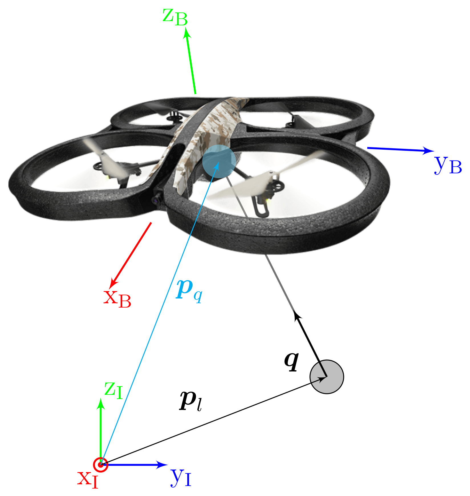
Consider a quadrotor attached to a load, assumed to be a point-mass, by a weightless rigid cable of length l, as illustrated in Figure 1. The inertial reference frames I of the quadrotor and load are handled with upward z and forward x. The positions of the load and quadrotor are denoted as and , respectively. The rotation matrix from the body fixed frame B, relative to I, is given by . The body-fixedframe angular velocities of the cable and quadrotor are denoted by and , respectively. The direction of the cable from the load position to the quadrotor position is given by the unit vector . The relation between the positions of the two bodies can be written as . Additionally, is restricted by . The masses of the load and quadrotor are and , respectively. The total mass of the system is . The inertia of the quadrotor in its body-fixedframe is and is positive definite.
The kinematic equations are
where is the skew-symmetric matrix of a vector . The skew-symmetric matrix is defined by the property that .
The formulation of the model in this paper follows the Lagrangian method presented in [11]. Therefore, the Lagrangian of the system is required. The kinetic energy of the system is
and the potential energy is
The resulting Lagrangian is , from which the system equations result:
where is the control force, f is the thrust, and is the input moment. The symbol represents the vector . The orthogonal projection of along is (a parallel component), and the orthogonal projection to the plane normal to is (a normal component). These projections are defined as
The objective of this paper was to provide an architecture with a hybrid-system-based trajectory that will be used for the control of a quadrotor transporting a cable-suspended load of unknown mass. Two components are used for the architecture: a trajectory generator and the controller. The architecture must transport the load from one point on the ground to another point on the ground, while also reaching a sufficient height, and with a mid-flight change in the load mass.
3. Control Architecture
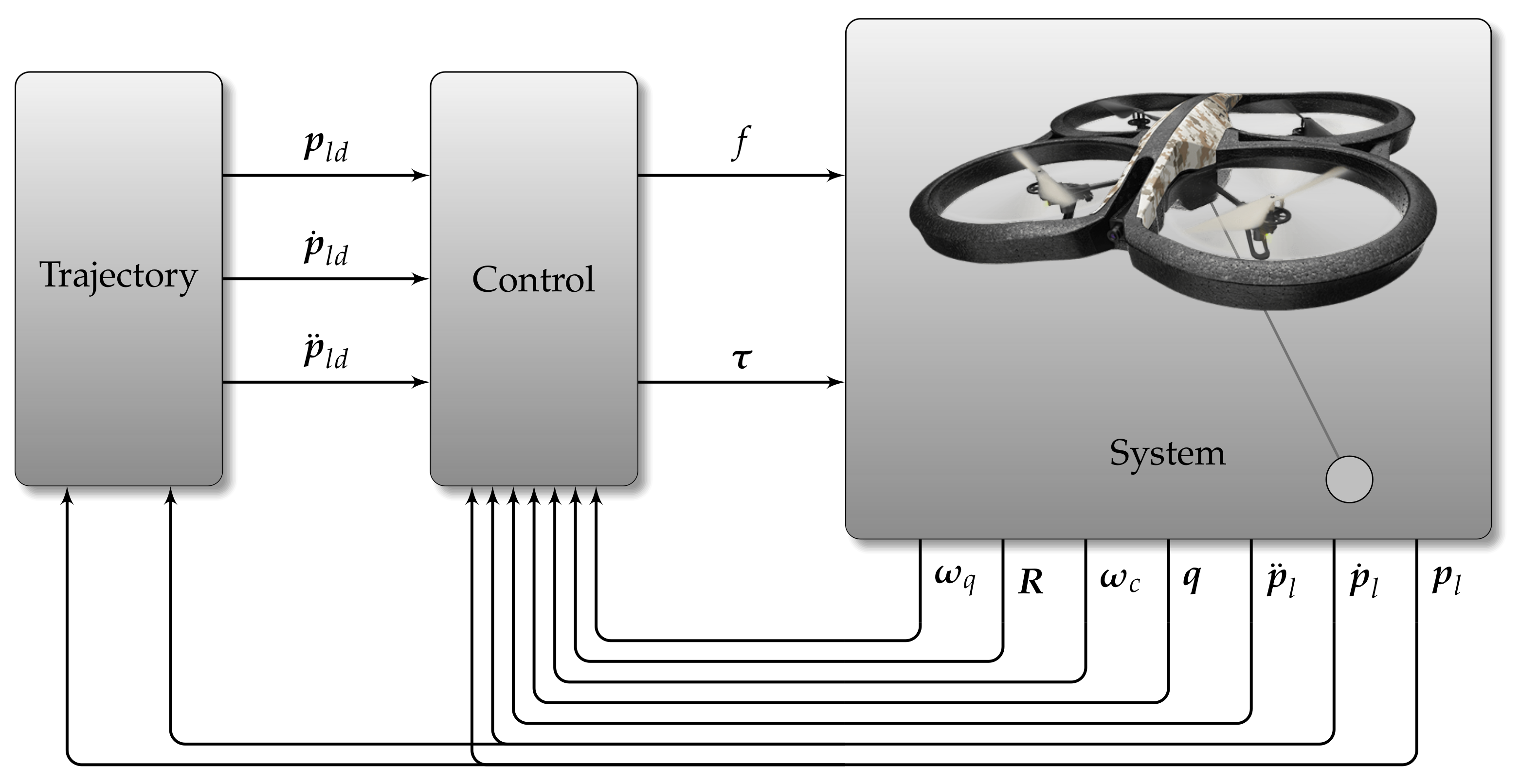
The proposed architecture is composed of a hybrid-automaton-based trajectory that provides position, velocity, and acceleration references to an adaptive geometric controller. The family of trajectories is designed to reflect the transportation of the load from one point on the ground to another. The control is responsible for the estimate of the load mass and tracking of the references provided by the trajectory. The architecture is presented in Figure 2.
4. Hybrid System Modeling
Hybrid systems [22] can be modeled according to different definitions: as a hybrid automaton, using hybrid behavior, and using event flow formulas. In this paper, the hybrid system presented is defined as a hybrid automaton:
Definition 1.
A generalized hybrid automaton is described by a six-tuple (L, X, A, W, R, ), where the symbols have the following meanings:
- L is a finite set, called the set of discrete states or locations. They are the vertices of a graph;
- X is the continuous state space of the hybrid automaton in which the continuous state variables x take their values. For our purposes, or X is an n-dimensional manifold;
- A is a finite set of symbols that serve to label the edges;
- is the continuous communication space in which the continuous external variables w take their values;
- R is a subset of ;
- Act is a mapping that assigns to each location a set of differential algebraic equations , relating the continuous state variables x to their time-derivatives and the continuous external variables w:The solutions of these differential-algebraic equations are called the activities of the location.
The subset R incorporates the notions of location invariants, guards, and jumps in the following way. To each location l, we associate the location invariant:
Furthermore, given two locations l, , we obtain the following guard for the transition from l to :
with the interpretation that the transition from l to l’ can take place if and only if . Finally, the associated jump relation is given by
5. Trajectory
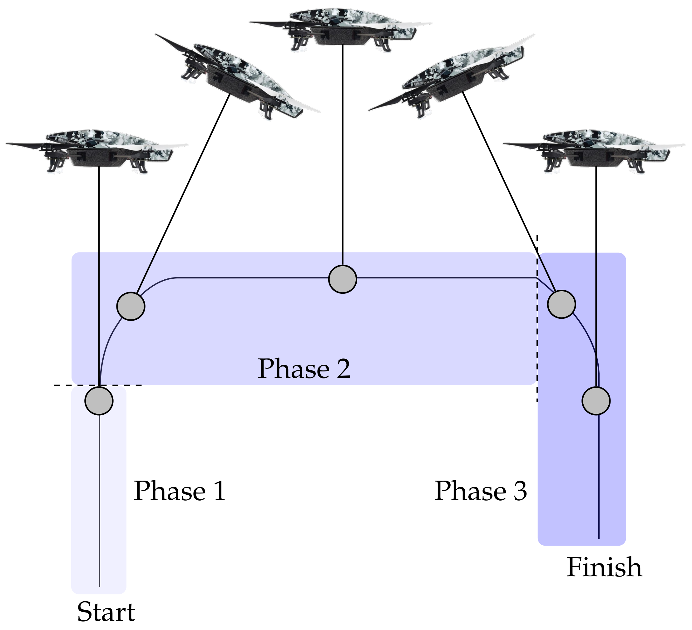
The proposed family of trajectories was chosen to provide references for the desired load position , velocity , and acceleration of the load. It was assumed that the quadrotor will maintain its x-vector facing forward. This section details the proposed family of trajectories and its implementation. The trajectories are divided into three phases, detailed in their respective subsections. The final subsection details the implementation. A representation of one of the trajectories is provided in Figure 3.
5.1. Phase 1—Lift-Off
During this initial phase, the quadrotor is requested to increase the load height at a constant rate, until it crosses a height threshold. After crossing the threshold, it switches to the second phase.
5.2. Phase 2—Transit
During this phase the quadrotor is requested to perform two tasks:
- Decelerate until the vertical velocity crosses the zero threshold and maintain zero vertical velocity afterwards;
- Accelerate until a specified forward velocity threshold is passed and maintain the specified forward velocity afterwards.
After a reaching a neighborhood of the desired endpoint, it switches to Phase 3.
5.3. Phase 3—Landing
During this phase, the quadrotor is requested to perform two tasks:
- Descend at a specified velocity until the load height threshold is reached, and, afterwards, reach zero vertical velocity and height;
- Decelerate until the forward velocity crosses the zero threshold, and then, hover above the endpoint.
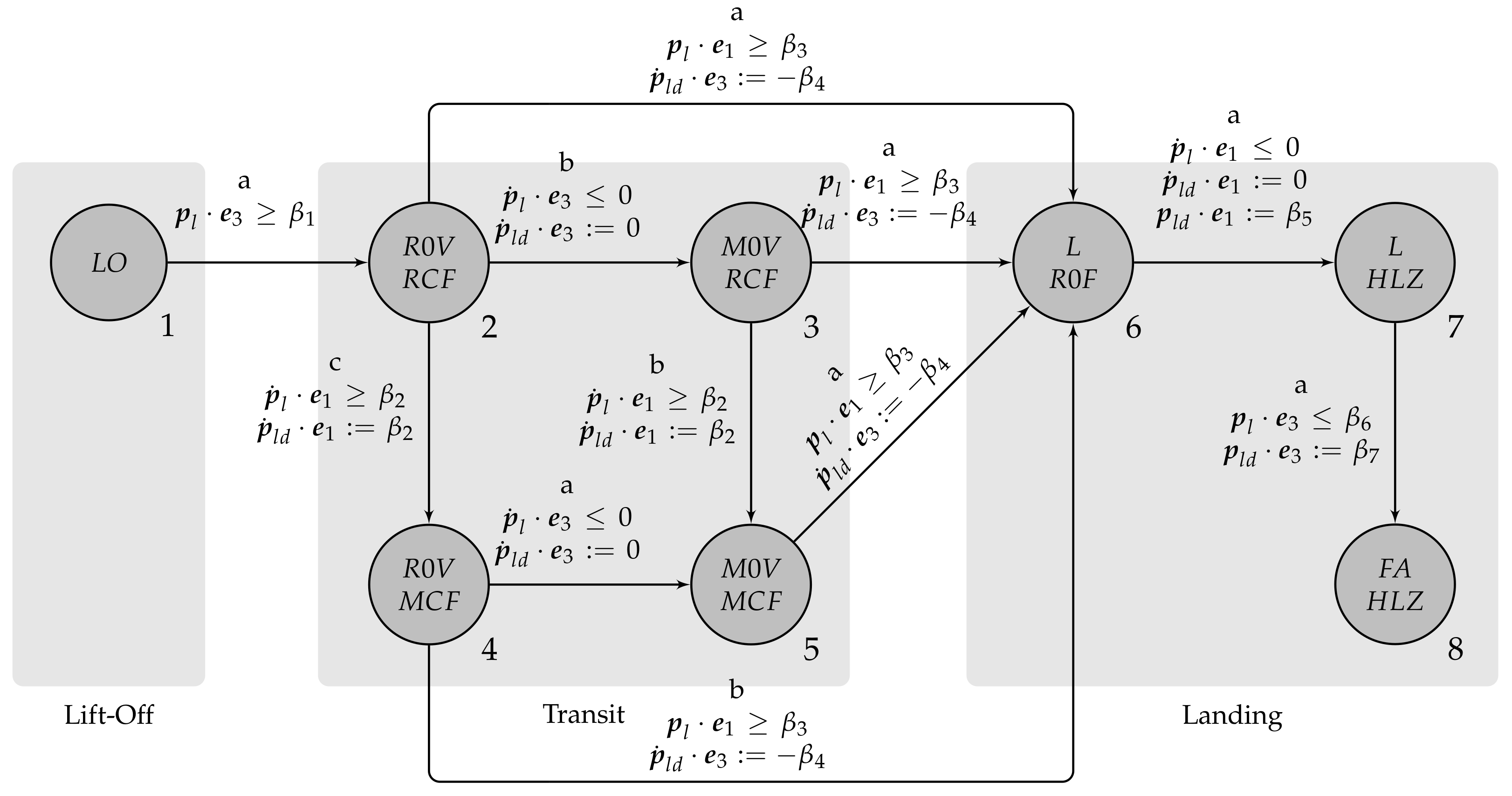
5.4. Hybrid System Implementation
The trajectory is provided by a hybrid model [22], whose diagram is shown in Figure 4. There are eight locations belonging to the set and (also numbered in Figure 4 from 1 to 8), composed of the behaviors in Table 1. It was assumed that the viability of the trajectory is maintained during testing.
Stage corresponds to the lift-off phase. Locations , , , and correspond to the transit phase. Locations , , and correspond to the landing phase. The state of the trajectory generator is the desired position and velocity of the load . The inputs of the generator are the position and velocity of the load .
The differential equations for the purpose of the desired experiment consist of, depending on the stage, some combination of constant acceleration, velocity, or position. Unless otherwise specified, the components of the acceleration are zero. has a constant upwards velocity and a constant x position; has a downwards acceleration, has a constant height, has a constant forward acceleration; has a constant forward velocity; L has a constant downward velocity; has a backwards acceleration; has a constant x position; has a constant height.
The edges of the system describe the possible transitions from stage l to . These are illustrated in Figure 4. Locations , , and can transition to for situations where the landing zone is very close to the lift-off point.
6. Control
This section details the control solution that will be used to test the trajectory. The control is first described assuming the load mass is known, providing a purely geometric controller. The required adjustment to provide an adaptive solution is discussed at the end of this section. The controller is divided into two components: the load control and the quadrotor control. The first component handles the desired behavior of the load, generating the requests to the quadrotor. These requests are sent to the quadrotor control, which handles the behavior of the quadrotor. The overall control is based on [11] (and the references therein) and [18].
6.1. Load Control
The first controller focuses on the load by ignoring the orientation of the quadrotor. Effectively, it was assumed that can be selected instantaneously. Since there are separate inputs for the position of the load () and the cable orientation (), as evidenced by (11) and (12), different control laws can be set for each component.
The component needs to adjust the gravitational acceleration of the load . Therefore, it is set as
where is a virtual control input. To ensure that this component remains parallel to , has to be parallel as well. Replacing (17) in (11) yields
The desired value of can now be designed. However, to ensure that it is parallel to , its desired value is first selected as
where is the position error, is the desired load position, is the position control gain, and is the velocity control gain. A parallel equivalent of is obtained using
To design the normal component of the control, it is necessary to establish what are the desired values of the direction of the cable and its angular velocity . Allowing the controller to define these, instead of an external trajectory generator, allows it to select values that are in agreement with the requests from the parallel component. For the case of the cable direction, holds important information and yields
The desired angular velocity is selected with the objective of achieving , which provides
To finish defining the normal input component, definitions of the errors of the direction of the cable and of the cable angular velocity are needed:
Additionally, (12) is rewritten as
The proposed formulation for is
where is the cable direction control gain and is the cable angular velocity control gain.
6.2. Quadrotor Control
The quadrotor controller is responsible for providing the desired force defined in the previous subsection by adjusting the thrust f and angular moments . Thus, a desired matrix for the orientation of the quadrotor is required. First, a value of the desired body z-axis can be obtained from :
Using a desired value of the body x-axis , which will be provided by the trajectory, the desired rotation matrix:
is obtained. The desired value for the angular velocity is obtained using the inverse map of a skew-symmetric matrix (, , ) according to
Having the desired values, the errors for the rotation matrix and the angular velocity can be defined as
The thrust is defined using the virtual control of the previous controller:
while the moments require the newly defined variables:
where is the rotation control gain, is the quadrotor angular velocity control gain, and is and additional control gain.
6.3. Adaptive Mechanism
In order for the presented controller to adapt to differences in the load mass, an adaptive mechanism [18] to adjust its outputs is required. Thus, an estimate of the load mass is deduced based on the desired gravitational acceleration and the errors of the position and velocity of the load. This way, the estimate can evolve based on how much the load is lagging behind the requested trajectory. The proposed mechanism is
This mechanism was selected because it preserves the tracking stability of the geometric solution, which will be shown in Appendix A.
Rewriting the relevant control equation from the previous sections, (19), to include the explicit estimate of the load mass results in
7. Simulation Results
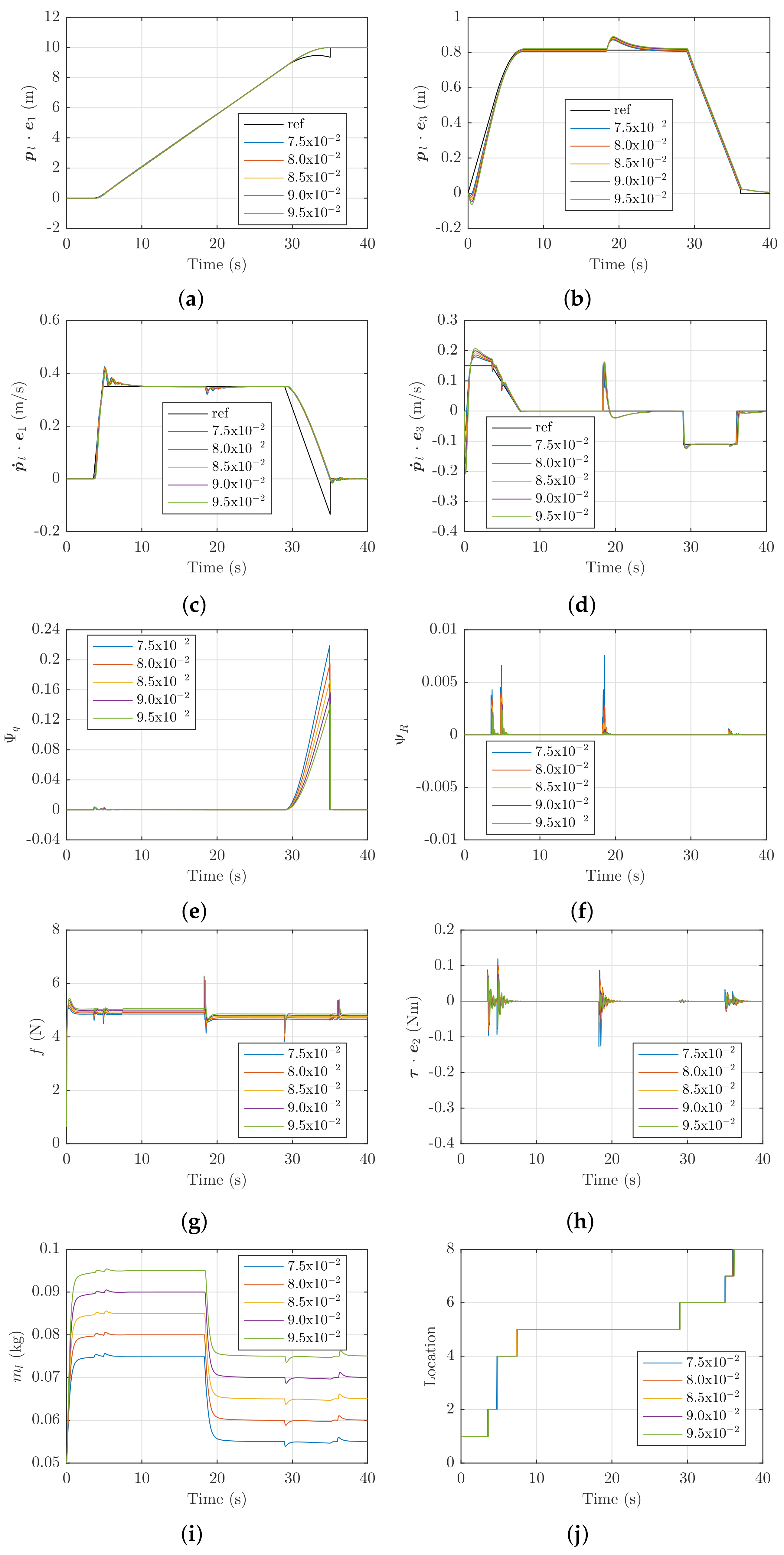
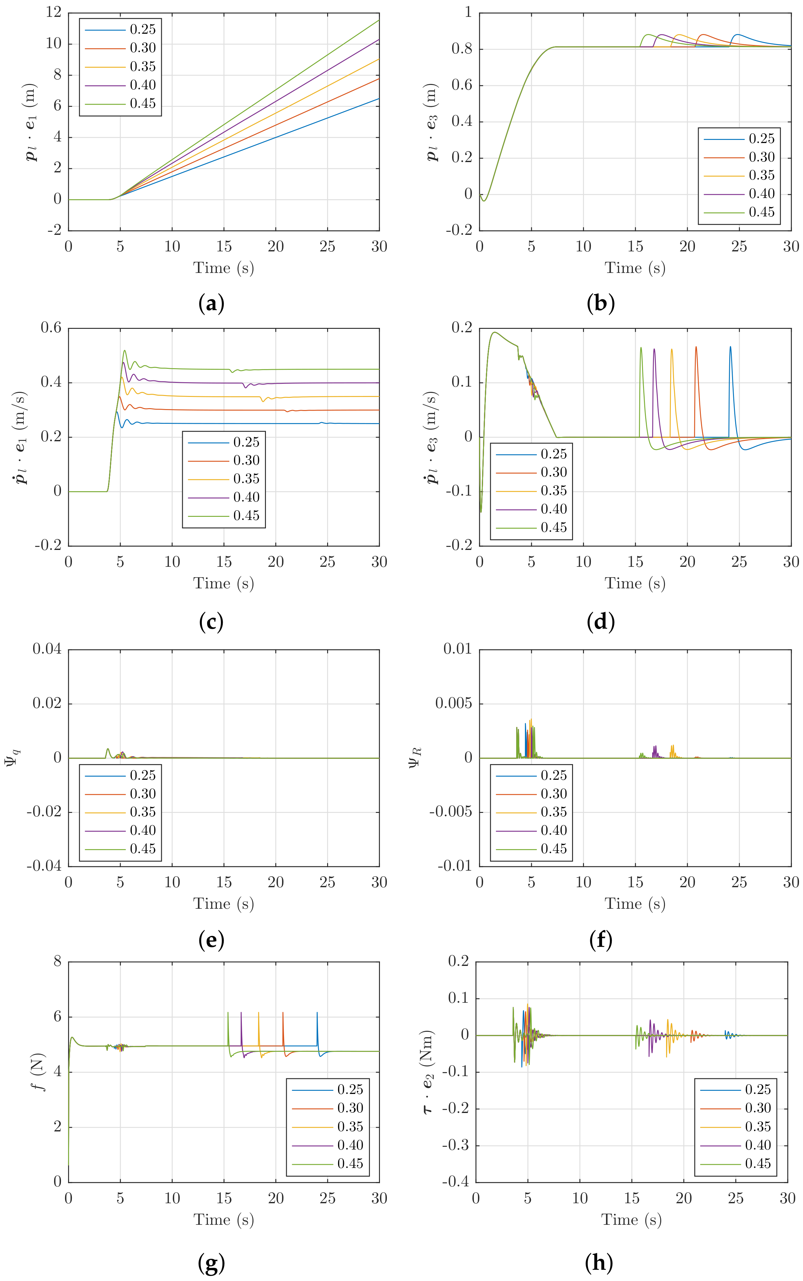
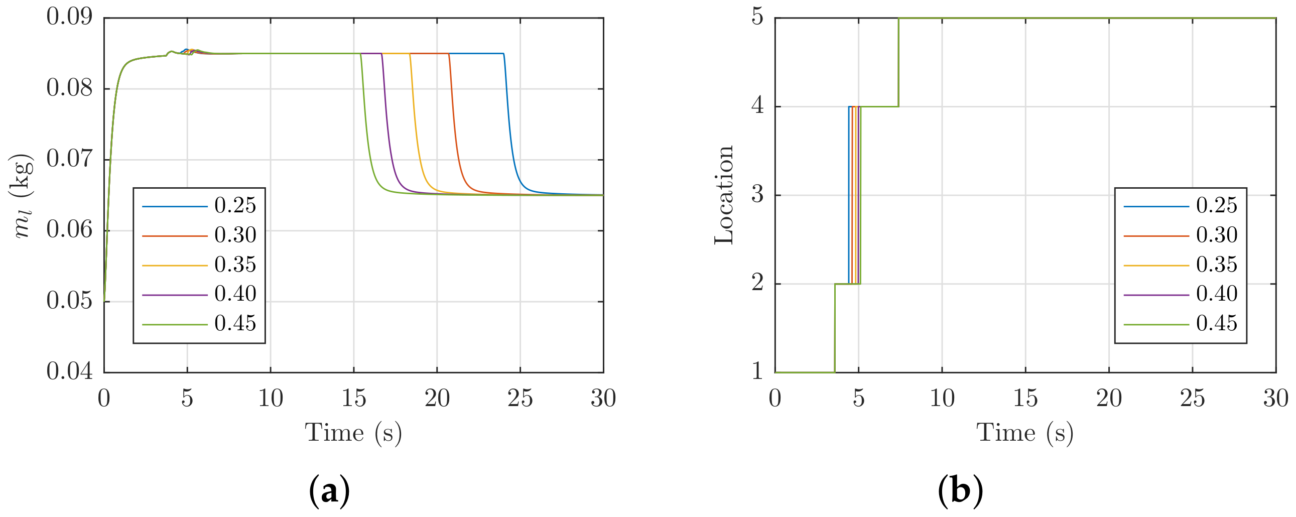
Two simulations were prepared to test the proposed solution. The parameters of the system are shown in Table 2. The control gains are presented in Table 3. The trajectory parameters are presented in Table 4. Some of these parameters were obtained by fine tuning. These parameters are provided for the sake of the reproducibility of the results. For plotting purposes, the locations of the trajectory are attributed an equivalent number: , as highlighted in Figure 4.
For the purpose of measuring the errors regarding and , the following metrics are proposed, respectively: and .
The first simulation included all phases of the trajectory. In this case, the mass of the load was tested at different values with a 0.02 kg (up to 4% of the total mass) drop after . The results of the simulation are presented in Figure 5, where the selected mass values are shown in the legend. The results were similar for all cases. The quadrotor was capable of following the trajectory in all locations of the trajectory, except , as evidenced by the rising error in Figure 5e and the delayed response in Figure 5c before the 34 s mark. The error observed in Figure 5b,d coincides with the mass estimate error at the start of the simulation and after the mass change. The forward velocity gains oscillation when there are changes to the requested velocity and to the load mass. This oscillation is dissipated, but remains for some time. For example, after the four-second mark (change in location ), it takes approximately four seconds to dissipate. The orientation of the quadrotor converges quickly to the desired value, as evidenced by the low peaks in the error measurement in Figure 5f. Lower load mass values lead to higher error measurements in Figure 5e,f. The thrust in Figure 5g is quick to respond and only presents a large peak when the mass change occurs. The moment is also quick to respond, only peaking when there are sudden changes in the requested orientation of the quadrotor. These request changes coincide with a change of location of the trajectory. The peaks of the moments are more pronounced for lower load masses. The mass estimate (Figure 5i) is also fast, converging with a settling time of two seconds to the real value at the start of the simulation and after the mass change. Additionally, the mass estimate has no overshoot, with sudden changes resulting from location changes. The largest values of the z velocity error in Figure 5d coincide with the points of larger mass estimation error.
The second simulation only included the first two phases. In this case, different maximum forward velocities were tested. The starting load mass was 0.085 kg and dropped 0.02 kg after . The results of the simulation are presented in Figure 6 and Figure 7, where the selected maximum forward velocity values are shown in the legend. The quadrotor is capable of moving at the desired maximum velocities, as evidenced in Figure 6c. Similar observations can be made for this simulation, when compared with the previous one, in regard to when the peaks and oscillations occur. Additionally, it was observed that identical behaviors occurred after the mass drop, even when traveling at different forward velocities, as highlighted in Figure 6b,d,g and Figure 7a. Very little error is observed in Figure 6e. The highest peaks after the mass drop in Figure 6f,h are observed for the 0.35 and 0.4 m/s cases, while the lowest peaks occur for the lowest velocity case.
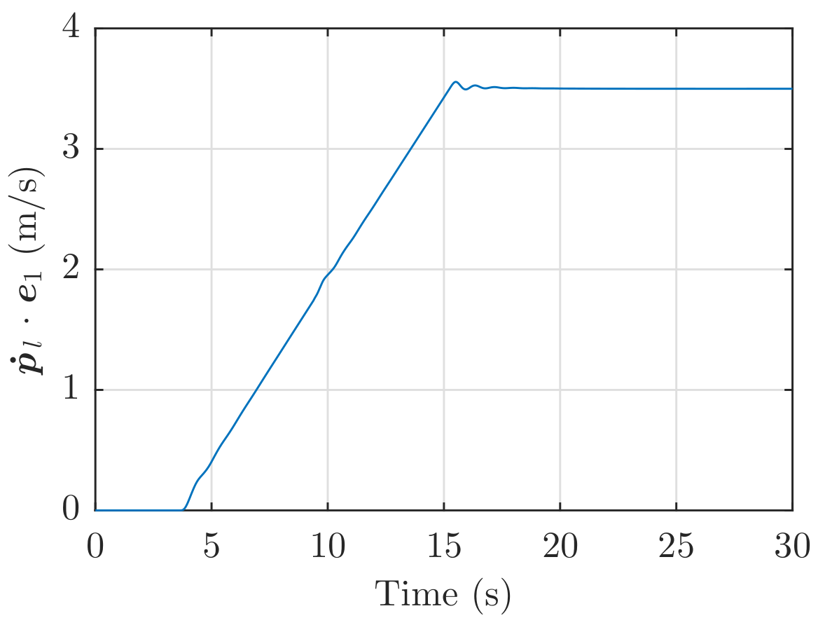
The controller performance was also tested for an increased maximum forward velocity scenario, away from the conservative nominal value. Figure 8 illustrates this scenario with a maximum forward velocity of 3.5 m/s (10-times more than the average value previously used. No discernible change was observed in the behavior of the velocity.
8. Conclusions
This paper proposed and validated an architecture for a quadrotor transporting a cable-suspended load of unknown mass from one point on the ground to another. A trajectory modeled as a hybrid system was proposed. An adaptive geometric control method with asymptotic tracking stability was used. The adaptive component of the control handles the mass uncertainty. The proposed system was tested in simulation with different load masses (between 0.075 and 0.095 kg) and maximum forward velocities (between 0.25 and 0.45 m/s), showing low settling times for the mass estimation and good tracking capabilities. The stability was verified in the simulation. Other effects, such as external disturbances (wind, rain, air density, among others) were considered as being rejected by the controller. These disturbances are being added to the model to design a more robust version of this control method in future work.
Author Contributions
P.O. (Pedro Outeiro): methodology, software, validation, writing—original draft. C.C. and P.O. (Paulo Oliveira): supervision, writing—review and editing, project administration, funding acquisition. All authors have read and agreed to the published version of the manuscript.
Funding
This work was financed by national funds through FCT—Foundation for Science and Technology, I.P., through IDMEC, under LAETA, Projects UIDB/50022/2020, CAPTURE (PTDC/EEIAUT/1732/2020), and POCI-01-0247-FEDER-046102, co-financed by Programa Operacional Competitividade e Internacionalização and Programa Operacional Regional de Lisboa, through Fundo Europeu de Desenvolvimento Regional (FEDER) and by National Funds through FCT—Fundação para a Ciência e Tecnologia. This work was also supported by FCT through the scholarship SFRH/BD/147035/2019.
Data Availability Statement
The data used in the present work is all available in the document itself.
Conflicts of Interest
The authors declare no conflict of interest.
Appendix A. Controller Stability
The stability of the control method hinges on the following theorem:
Theorem A1.
The proposed controller provides an asymptotically stable zero equilibrium of tracking errors, so long as the selected trajectory ensures that
The proof of Theorem A1 hinges on showing that there is a set of trajectories that can be requested from the system, for which the system is stable. For this, the error dynamics have to be examined first. From Equations (18) and (20) results
which can be adjusted as follows:
In these equations, represents the error associated with the difference between and , and it is given by
Equation (21) dictates that , which allows writing as a function of :
An upper bound of can be obtained as
for some positive constant B, which depends on the desired trajectories of the load.
The next step of the proof requires a Lyapunov function to show the tracking stability. First, a cable configuration error function that is positive definite around is defined as
For positive constants , consider the following open domain containing the zero equilibrium of tracking error variables:
In this domain, . It can be shown that the cable configuration error is quadratic with respect to the error vectors in the sense that
where the upper bounds are satisfied only in the domain D.
The Lyapunov function is defined as
where , are positive constants and is the mass estimate error. The derivative of (A14) is
Let , . The Lyapunov function satisfies
where the matrices , , , and are given by
If the constants , are sufficiently small, all of the above matrices are positive definite. It follows that the Lyapunov function is positive definite.
From (A10), an upper-bound of the fourth element of is given by
Substituting this into (A15) and rearranging, is bounded by
where , and the matrix is defined as
where is the minimum eigenvalue of ; the sub-matrices are given by:
If the constants , , which are independent of the control input, are sufficiently small, the matrices , are positive definite. Furthermore, if the error in the direction of the cable is sufficiently small (determined by constant B) relative to the desired trajectory in Section 5.4, the controller gains can be chosen such that the matrix W is positive definite. Since does not include the mass estimate, it is necessary to analyze to finalize the stability proof.
is bounded, as shown in (A10). Its derivative is also bounded. is provided by the proposed trajectory, which ensures it is bounded. Therefore, is bounded, and is uniformly continuous in and negative definite. From Barbalat’s lemma, it follows that the zero equilibrium of tracking errors is asymptotically stable.
The proof of the stability of the controller in Section 6.2 is provided in Annex C. of [23], therefore proving that Theorem A1 is correct.
References
- UPS Partners with Matternet to Transport Medical Samples via Drone across Hospital System in Raleigh, N.C. Available online: https://pressroom.ups.com/pressroom/ContentDetailsViewer.page?ConceptType=PressReleases&id=1553546776652-986 (accessed on 16 April 2019).
- Amazon Prime Air Website. Available online: https://www.amazon.com/Amazon-Prime-Air/b?node=8037720011 (accessed on 16 April 2019).
- Arshad, M.A.; Ahmed, J.; Bang, H. Quadrotor Path Planning and Polynomial Trajectory Generation Using Quadratic Programming for Indoor Environments. Drones 2023, 7, 122. [Google Scholar] [CrossRef]
- Al Younes, Y.; Barczyk, M. Adaptive Nonlinear Model Predictive Horizon Using Deep Reinforcement Learning for Optimal Trajectory Planning. Drones 2022, 6, 323. [Google Scholar] [CrossRef]
- Zhang, Z.; Li, J.; Wang, J. Sequential convex programming for nonlinear optimal control problems in UAV path planning. Aerosp. Sci. Technol. 2018, 76, 280–290. [Google Scholar] [CrossRef]
- He, L.; Aouf, N.; Song, B. Explainable Deep Reinforcement Learning for UAV autonomous path planning. Aerosp. Sci. Technol. 2021, 118, 107052. [Google Scholar] [CrossRef]
- Shin, Y.; Kim, E. Hybrid path planning using positioning risk and artificial potential fields. Aerosp. Sci. Technol. 2021, 112, 106640. [Google Scholar] [CrossRef]
- Baca, T.; Hert, D.; Loianno, G.; Saska, M.; Kumar, V. Model Predictive Trajectory Tracking and Collision Avoidance for Reliable Outdoor Deployment of Unmanned Aerial Vehicles. In Proceedings of the 2018 IEEE/RSJ International Conference on Intelligent Robots and Systems (IROS), Madrid, Spain, 1–5 October 2018; pp. 6753–6760. [Google Scholar] [CrossRef]
- Sreenath, K.; Michael, N.; Kumar, V. Trajectory generation and control of a quadrotor with a cable-suspended load-A differentially-flat hybrid system. In Proceedings of the 2013 IEEE International Conference on Robotics and Automation, Karlsruhe, Germany, 6–10 May 2013; pp. 4888–4895. [Google Scholar] [CrossRef]
- Sreenath, K.; Lee, T.; Kumar, V. Geometric control and differential flatness of a quadrotor UAV with a cable-suspended load. In Proceedings of the 52nd IEEE Conference on Decision and Control, Firenze, Italy, 10–13 December 2013; pp. 2269–2274. [Google Scholar]
- Lee, T. Geometric control of multiple quadrotor UAVs transporting a cable-suspended rigid body. In Proceedings of the 53rd IEEE Conference on Decision and Control, Los Angeles, CA, USA, 15–17 December 2014; pp. 6155–6160. [Google Scholar] [CrossRef] [Green Version]
- Dai, S.; Lee, T.; Bernstein, D.S. Adaptive control of a quadrotor UAV transporting a cable-suspended load with unknown mass. In Proceedings of the 53rd IEEE Conference on Decision and Control, Los Angeles, CA, USA, 15–17 December 2014; pp. 6149–6154. [Google Scholar] [CrossRef]
- Notter, S.; Heckmann, A.; Mcfadyen, A.; Gonzalez, L. Modelling, Simulation and Flight Test of a Model Predictive Controlled Multirotor with Heavy Slung Load. IFAC-PapersOnLine 2016, 49, 182–187. [Google Scholar] [CrossRef] [Green Version]
- Yang, S.; Xian, B. Energy-Based Nonlinear Adaptive Control Design for the Quadrotor UAV System With a Suspended Payload. IEEE Trans. Ind. Electron. 2020, 67, 2054–2064. [Google Scholar] [CrossRef]
- Bingöl, O.; Güzey, H.M. Finite-Time Neuro-Sliding-Mode Controller Design for Quadrotor UAVs Carrying Suspended Payload. Drones 2022, 6, 311. [Google Scholar] [CrossRef]
- Xu, R.; Ozguner, U. Sliding Mode Control of a Quadrotor Helicopter. In Proceedings of the 45th IEEE Conference on Decision and Control, San Diego, CA, USA, 13–15 December 2006; pp. 4957–4962. [Google Scholar]
- Lee, T. Robust Adaptive Attitude Tracking on SO(3) with an Application to a Quadrotor UAV. IEEE Trans. Control Syst. Technol. 2013, 21, 1924–1930. [Google Scholar]
- Song, J.; Chang, D.E.; Eun, Y. Passivity-based Adaptive Control of Quadrotors with Mass and Moment of Inertia Uncertainties. In Proceedings of the 2019 IEEE 58th Conference on Decision and Control (CDC), Nice, France, 11–13 December 2019; pp. 90–95. [Google Scholar]
- Dydek, Z.T.; Annaswamy, A.M.; Lavretsky, E. Adaptive Control of Quadrotor UAVs: A Design Trade Study with Flight Evaluations. IEEE Trans. Control Syst. Technol. 2013, 21, 1400–1406. [Google Scholar] [CrossRef]
- Outeiro, P.; Cardeira, C.; Oliveira, P. MMAC Height Control System of a Quadrotor for Constant Unknown Load Transportation. In Proceedings of the 2018 IEEE/RSJ International Conference on Intelligent Robots and Systems (IROS), Madrid, Spain, 1–5 October 2018; pp. 4192–4197. [Google Scholar] [CrossRef]
- Roy, S.; Baldi, S.; Li, P.; Narayanan, V. Artificial-Delay Adaptive Control for Under-actuated Euler-Lagrange Robotics. IEEE/ASME Trans. Mechatron. 2021, 26, 3064–3075. [Google Scholar] [CrossRef]
- Van Der Schaft, A.; Schumacher, H. An Introduction to Hybrid Dynamical Systems; Springer: London, UK, 2000. [Google Scholar]
- Lee, T. Geometric Control of Multiple Quadrotor UAVs Transporting a Cable-Suspended Rigid Body. arXiv 2014, arXiv:1403.3684. [Google Scholar]
Figure 1.
Quadrotor with cable-suspended load.

Figure 2.
Control architecture (—desired load position).

Figure 3.
Trajectory example (not to scale).

Figure 4.
Trajectory hybrid system diagram ().

Figure 5.
Simulation results for different load masses (). (a) x position. (b) z position. (c) x velocity. (d) z velocity. (e) error. (f) error. (g) thrust. (h) y moment. (i) Mass estimate. (j) Location number (refer to Figure 4).
Figure 5.
Simulation results for different load masses (). (a) x position. (b) z position. (c) x velocity. (d) z velocity. (e) error. (f) error. (g) thrust. (h) y moment. (i) Mass estimate. (j) Location number (refer to Figure 4).

Figure 6.
Simulation results for different maximum forward velocities (). (a) x position. (b) z position. (c) x velocity. (d) z velocity. (e) error. (f) error. (g) thrust. (h) y moment.
Figure 6.
Simulation results for different maximum forward velocities (). (a) x position. (b) z position. (c) x velocity. (d) z velocity. (e) error. (f) error. (g) thrust. (h) y moment.

Figure 7.
Simulation results for different maximum forward velocities: continued from Figure 6. (a) Mass estimate. (b) Location number (refer to Figure 4).

Figure 8.
Simulation forward velocity results for increased maximum velocity (3.5 m/s).


Table 1.
Location behaviors.
| Abbreviation | Name | Diff. Equation |
|---|---|---|
| Lift-Off | ||
| Reach Zero Vertical Velocity | ||
| Maintain Zero Vertical Velocity | ||
| Reach Cruise Forward Velocity | ||
| Maintain Cruise Forward Velocity | ||
| L | Landing | |
| Reach Zero Forward Velocity | ||
| Hover Landing Zone | ||
| Final Approach |
Table 2.
System parameters.
| Parameter | Value |
|---|---|
| (kg) | 0.42 |
| (kg m2) | |
| (kg m2) | |
| (kg m2) | |
| l (m) | 0.75 |
Table 3.
Control gains.
| Gain | Value |
|---|---|
| 0.5 | |
| 0.9 | |
| 0.125 | |
| 3 | |
| 0.02 | |
| 0.5 | |
Table 4.
Trajectory parameters.
| Parameter | Value |
|---|---|
| 0.5 | |
| 0.35 | |
| 8.7 | |
| 0.11 | |
| 10 | |
| 0 | |
| 0.15 | |
| 0.04 | |
Disclaimer/Publisher’s Note: The statements, opinions and data contained in all publications are solely those of the individual author(s) and contributor(s) and not of MDPI and/or the editor(s). MDPI and/or the editor(s) disclaim responsibility for any injury to people or property resulting from any ideas, methods, instructions or products referred to in the content. |
© 2023 by the authors. Licensee MDPI, Basel, Switzerland. This article is an open access article distributed under the terms and conditions of the Creative Commons Attribution (CC BY) license (https://creativecommons.org/licenses/by/4.0/).
Share and Cite
MDPI and ACS Style
Outeiro, P.; Cardeira, C.; Oliveira, P. Control Architecture for a Quadrotor Transporting a Cable-Suspended Load of Uncertain Mass. Drones 2023, 7, 201. https://doi.org/10.3390/drones7030201
AMA Style
Outeiro P, Cardeira C, Oliveira P. Control Architecture for a Quadrotor Transporting a Cable-Suspended Load of Uncertain Mass. Drones. 2023; 7(3):201. https://doi.org/10.3390/drones7030201
Chicago/Turabian StyleOuteiro, Pedro, Carlos Cardeira, and Paulo Oliveira. 2023. "Control Architecture for a Quadrotor Transporting a Cable-Suspended Load of Uncertain Mass" Drones 7, no. 3: 201. https://doi.org/10.3390/drones7030201