
Carrier Aircraft Flight Controller Design by Synthesizing Preview and Nonlinear Control Laws

School of Aeronautic Science and Engineering, Beihang University, Beijing 100191, China
*
Author to whom correspondence should be addressed.
Drones 2023, 7(3), 200; https://doi.org/10.3390/drones7030200
Submission received: 23 February 2023
/
Revised: 13 March 2023
/
Accepted: 14 March 2023
/
Published: 15 March 2023
Abstract
:This paper proposes an innovative automatic carrier landing control law for carrier-based aircraft considering complex ship motion and wind environment. Specifically, a strategy is proposed to synthesize preview control with an adaptive nonlinear control scheme. Firstly, incremental nonlinear backstepping control law is adopted in the attitude control loop to enhance the anti-disturbance capability of the aircraft. Secondly, to enhance the glide slope tracking performance under severe sea conditions, the carrier motion is predicted, and the forecasted motion is adopted in an optimal preview control guidance law to compensate influences induced by carrier motion. However, synthesizing the inner-loop and outer-loop control is not that straightforward since the preview control is naturally an optimal control law which requires a state-space model. Therefore, low-order equivalent fitting of the attitude-to-altitude high-order system model needs to be performed; furthermore, a state observer needs to be designed for the low-order equivalent system to supply required states to the landing controller. Finally, to validate the proposed methodology, an unmanned tailless aircraft model is used to perform the automatic landing tasks under variant sea conditions. Results show that the automatic carrier landing system can lead to satisfactory landing precision and success rate even under severe sea conditions.
1. Introduction
Precisely landing carrier aircraft on a small area of the moving carrier under severe marine conditions is a significant challenge. In order to accomplish the all-weather operation of carrier aircraft under complex sea conditions, such as strong deck motion and high air wake, it is essential to design an advanced automatic carrier landing system (ACLS). The key factors influencing the landing safety and precision of the aircraft system can be typically classified into two types: internal model uncertainties and external disturbances. On one hand, the control surface/actuator faults are usually sudden changes occurring to the aircraft, and can be classified into the uncertainties of the aircraft model. On the other hand, air wakes and sea condition changes could be viewed as external environment disturbances.
The guidance and control problem of automatic carrier landing has been widely studied since the middle of the 20th Century. According to the literature, ACLSs based on conventional control methods [1,2,3], such as PID, have been used in practice for a long time. Furthermore, there exist many ACLS design methods which are based on linearized models; for example, the optimal control method [4], the H∞ control method [5,6], stochastic model predictive control [7], and optimal preview control methods [8,9]. Recently, artificial intelligence has also been used in autonomous unmanned aerial vehicle control [10,11,12]. However, the control performance of these abovementioned methods will inevitably decrease when the model is mismatched or the aircraft suffer from strong disturbances.
Scholars have widely investigated how to improve the anti-disturbance ability of flight controllers for carrier aircraft under uncertain disturbances. Ref. [13] proposed an adaptive super-twisting controller for ACLSs, and the unmatched uncertainties caused by air wake were considered. In Ref. [14], a model reference adaptive control method was developed based on system linearization. In Ref. [15], an ACLS was designed based on active disturbance rejection control (ADRC), and an extended state observer (ESO) was used to observe the comprehensive disturbances for compensation. In Ref. [16], a nonlinear fixed-time control method was developed for ACLS design, where observers were introduced to deal with disturbances. Prescribed performance controllers for automatic carrier landing were presented in Refs. [17,18], and a disturbance observer was developed to observe the disturbances. In addition to the abovementioned adaptive control methods, incremental nonlinear control (INC) laws have also been proven to be effective methods to achieve disturbance rejection [19,20,21]. Through the acceleration measurements or the estimation of the state derivatives, this type of methods can quickly feedback the dynamic changes of the system to the controller. At the same time, compared with the traditional model-based nonlinear control laws, e.g., a classical dynamic inversion controller, as in Ref. [22], INC has less model dependency, stronger adaptation capability, and fault accommodation capability. It can be deduced that the application of incremental nonlinear control is helpful to improve the anti-disturbance capability of carrier-aircraft inner loop attitude controllers.
In complex sea conditions, the movement of the carrier can usually lead to phase lag of the guidance laws, which therefore significantly reduces the landing accuracy. In order to reduce the influences of carrier motion, scholars have proposed a number of methods in the literature. For example, for the longitudinal height control, a common method has been to use the linear leading filter to correct the phase in the frequency domain [18,23]. Similarly, a tracking differentiator was used to realize the function of leading filter in Ref. [15]. In these two methods, the correction ability of the leading filter was limited; that is, these two controllers can only compensate the influence of the deck motion to a certain extent. Another common method in research is to predict the carrier motion in the time domain. For example, in Refs. [13,14], a particle filter was used to predict the carrier motion for a fixed time point in the future time window, e.g., the time point for 2 s later, to calculate the future altitude commands. Therefore, the carrier aircraft can track the future command, through which the phase delay induced by the deck motion is compensated for. This type of method assumes that the phase lag of the guidance law is fixed under certain carrier motion. However, when changes occur to the speed of the carrier, the sea conditions, and the characteristics of the carrier aircraft, the phase lag will accordingly change. Consequently, the influence of the carrier motion is usually partially compensated if the carrier aircraft track command signals at a fixed future time point, as is the case in the abovementioned methods.
Optimal preview control (OPC) has the capability to effectively compensate the system delay by using the future command information. For example, when the terrain ahead is known, it can achieve high-precision terrain tracking [24,25,26]. Considering the characters of the carrier motion, e.g., periodicity and randomness, the carrier motion can also be predicted. This predicted information can then be viewed as future commands, and is then fed to the optimal preview controller. In recent years, Zhen et al. extended the application of the OPC for the purpose of carrier landing controller design [8,9]. The results showed that the optimal preview control could effectively compensate for the motion of the carrier, and the landing precision was correspondingly improved. Although this method also needs to predict the future movements of the carrier, it does not need to know the exact lag time of the guidance control system. Specifically, the carrier motion sequences in the future time window are used to compensate the carrier motion in the framework of optimal preview control. However, OPC requires a linear state-space model of the controlled plants, and its control performance will decrease if evident model mismatch exists.
In order to achieve effective compensation of carrier motion and high anti-disturbance performance in automatic carrier landing tasks, a novel control method for ACLSs is proposed by synthesizing the optimal preview control and adaptive nonlinear controller. More precisely, an optimal preview guidance law is designed in the outer loop to effectively compensate for the motion of the carrier. At the same time, an attitude controller is designed using incremental adaptive nonlinear control law in the inner loop to improve the disturbance rejection ability of the system. Different from the existing literature, the main contributions of this paper are summarized as follows:
- (1)
- The optimal preview control-based guidance law and adaptive nonlinear control law are synthesized to propose a novel automatic carrier landing system. On one hand, the optimal preview control is used in the guidance loop to actively/effectively compensate for the deck motion. On the other hand, an incremental type adaptive nonlinear control law is used to design the attitude controller considering model uncertainties or external disturbances. The synthesis of the inner-loop nonlinear attitude controller design and the preview control-based outer-loop glide slope guidance law is not straightforward because preview control is naturally an optimal control law, which requires a state-space model of the controlled plant. In the existing literature, there are no researches on how to synthesize these two types of methods. Different from the OPC design in Refs. [8,9], the proposed method does not depend on linearized high-order models. Compared to the ACLS designed based on nonlinear or adaptive control laws [13,14,15,16,17,18], the proposed method actively fulfills flight deck motion prediction and compensation.
- (2)
- In order to allow that the optimal preview control method is used to design the outer-loop guidance law, an attitude-to-altitude linearization scheme including the necessary associated techniques is developed. Specifically, a low-order equivalent fitting method is used to linearize the attitude-to-altitude system, where the inner loop consists of an attitude controller. A state observer is developed for estimating the states required by the low-order equivalent linear model. Furthermore, a neural network forecasting model is developed to predict the deck motion.
- (3)
- Several typical simulation scenarios are simulated to verify the guidance control system designed in this paper. Compared to a classical landing controller using the PID guidance law and the PID attitude control law, and the OPC guidance-law-based landing controller from Refs. [8,9], the designed controller can effectively circumvent the phase lag problem caused by the deck motion, and has strong adaptive ability in the face of model uncertainties and sudden disturbances.
The remainder of this paper is organized as follows. The second section describes the landing control problem of carrier aircraft and introduces the landing controller design based on the incremental sliding mode control law and the PID guidance law. The third section gives the design method for the guidance law using the preview control. Simulation results and analysis are given in the fourth section. Finally, section five concludes this paper.
2. Problem Statement for Automatic Landing and Baseline Guidance and Attitude Controller Design
This section first provides the models of the aircraft, the carrier, and the air wakes, which provide the basis for the design of automatic landing controller. Then, the general guidance and control framework is given.
2.1. Carrier Aircraft/Carrier and Air Wake Modeling
2.1.1. Carrier Aircraft Modeling
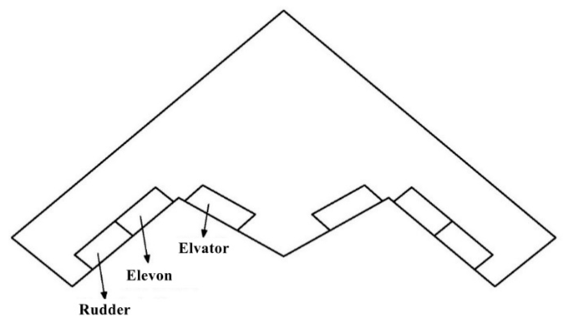
The carrier aircraft used in this paper is a tailless flying-wing aircraft. The geometric and inertial data are obtained from the EQ model presented in Ref. [27], and the aerodynamic data are obtained from the EQII model, as in Ref. [28]. Because the geometric data of the EQII model and the EQ model are similar, the Reynolds numbers are also close, so the aerodynamic data of the EQII model can be used to represent the aerodynamics of the EQ model. The shape of the EQ model is shown in the following Figure 1.
The dynamics and kinematics of the aircraft can be described by the following equations:
where , , are the force on the aircraft in the body-fixed frame;, , are the speed in the body-fixed frame., , are the Euler angles; , , are the angular acceleration; , , are the moments in the body-fixed frame; , , are the moment of inertia; represents the product of inertia with respect to the Oz and Ox axes., , are position in the earth-fixed frame; represents the transformation matrix from the body-fixed frame to the earth-fixed frame.
The aerodynamic coefficients of the aircraft can be found in Ref. [28].
where , , are the drag, side force, and lift coefficients; represents the wing span and c represents the mean aerodynamic chord.
2.1.2. Carrier Modeling
The motion of the carrier is mainly composed of two parts. One is its basic motion, the other part is the disturbance motion added on to the basic motion, including translational disturbances (surge, sway, and heave) and rotational disturbances (roll, pitch, and yaw). The basic motion can be regarded as the motion of the mass center of the carrier.
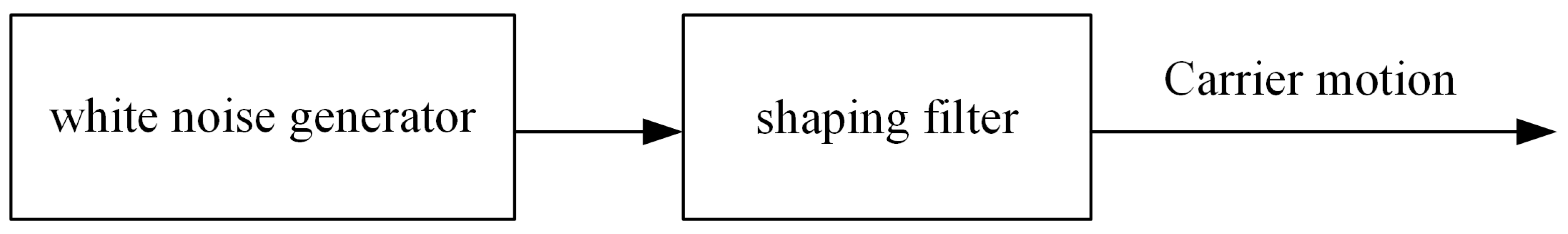
For the disturbance motion, there are two kinds of modeling methods in practice. The first kind of method assumes that the disturbance motion is a combination of several harmonics. This model is a little bit ideal and cannot fully reflect the random and uncertain characteristics of the carrier motion. In the second kind of method, the carrier motion is assumed to be a stationary random process with a narrow bandwidth [30,31,32]; therefore, the carrier motion is constructed based on the power spectral density functions. This method is more practical since it can well reflect the randomness of the motion. The shaping filter can be expressed using the following two transfer functions, see Equations (7) and (8), where represents the translational disturbances shaping filter, and represents the rotational disturbances shaping filter. Then, the detailed forms and parameters of the shaping filter functions affecting the longitudinal motion of the aircraft carrier are given in Table 2, and the motion generation method is illustrated in Figure 2.
2.1.3. Air Wake Model
The modeling method for the atmospheric disturbances faced by carrier-based aircraft during landing is given in the U.S. military standard [33]. It consists of four parts: a free atmospheric turbulence component , a steady wake component , a periodic wake component and a random wake component . Then, the final wind field can be expressed as follows:
2.2. Overall Control Structure for Automatic Landing Controller
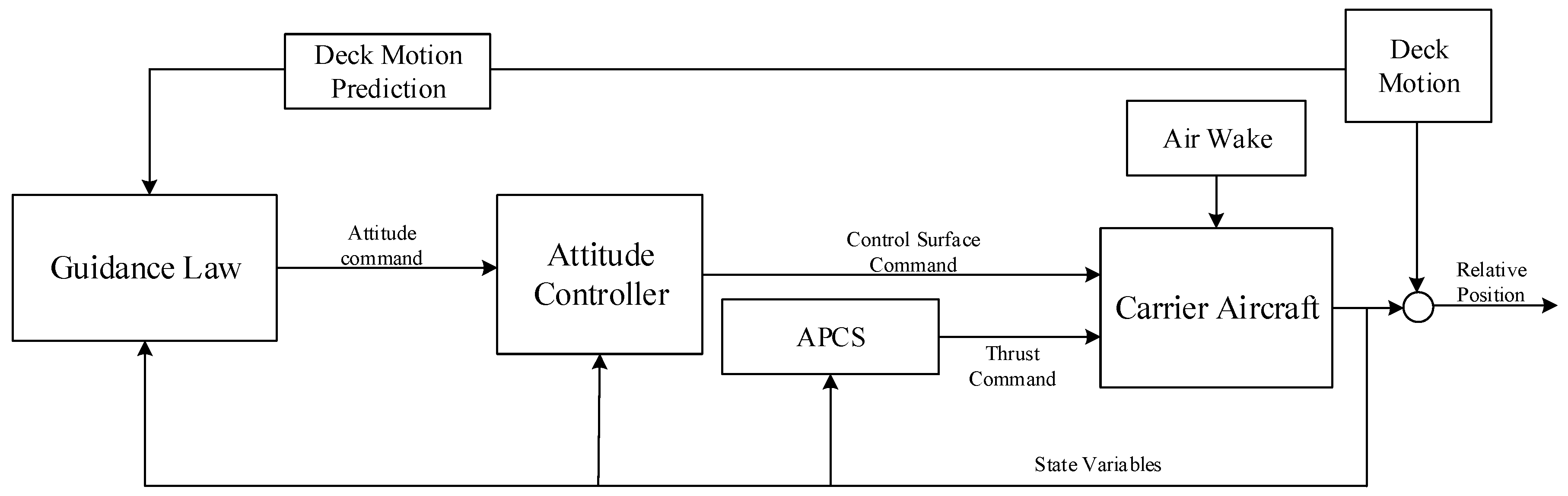
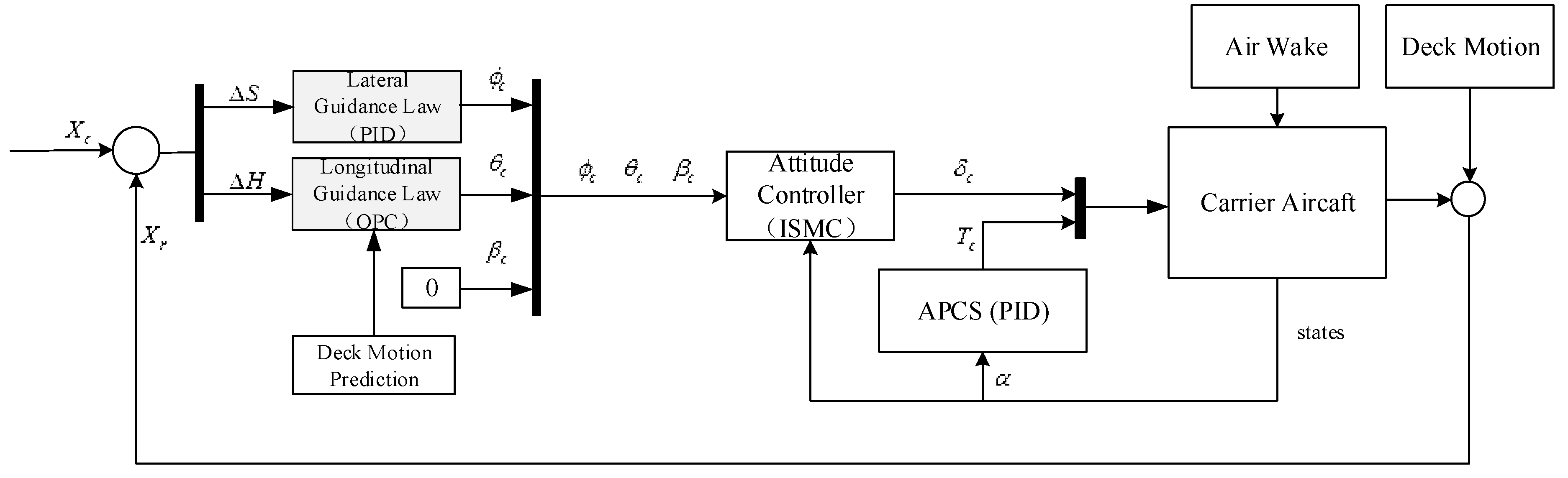
The carrier landing controller usually consists of an inner loop and an outer loop. The outer loop consists of the guidance law, which generates the attitude commands for the inner loop. The inner loop consists of an attitude controller and an approach power compensation system (APCS). The function of the inner loop is designed to control attitude and maintain the angle of attack, respectively. The structure of the overall control system is shown in Figure 3.
As shown in Figure 3, air wake disturbances and deck motions are two key factors that will influence the landing control performance of the carrier aircraft. Furthermore, the influence of model uncertainty cannot be ignored. In order to reduce the influence of internal model uncertainties and external environment disturbances, an attitude controller with strong anti-disturbance capability is designed in Section 3. In order to reduce the influence caused by deck motion, the guidance law considering deck motion compensation is developed in Section 4.
2.3. Incremental Sliding Mode Attitude Controller and PID Guidance Law
In the attitude controller design, both the internal model uncertainties and the external wind disturbances need to be considered. In addition, the control method is usually expected to have low-level model dependency considering the difficulties in obtaining a highly accurate model of the carrier aircraft. Considering the abovementioned factors, this paper adopts the incremental sliding mode control (ISMC) method to design a high-performance attitude controller. This method inherits both the advantages of the sliding mode control law and that of the incremental nonlinear control method, and it has strong disturbance rejection capability and low model dependency. In this paper, the carrier aircraft is modeled as a second-order system with strict feedback form. Subsequently, the design method for the second-order incremental sliding mode controller is introduced.
2.3.1. Incremental Model for Attitude Controller Design
The angular motion equations of carrier aircraft can be written as follows:
where , , is the synthesized disturbance and is assumed to be bounded.
Suppose that the state variable at the time is denoted by the subscript 0, then Equation (10b) can be rewritten as an incremental form for the time moment:
where .
Then, the Taylor expansion of Equation (10b) at can be obtained:
By substituting Equation (11) into Equation (12), it is obtained that
where , and note that has been assumed to be very small since the sampling frequency is usually relatively high; e.g., equal to or larger than 50 Hz.
Finally, Equation (10a) can be differentiated as an incremental second-order model for controller design:
For the command tracking problem, the error dynamics are expressed as follows:
where is the desired output, and is output error vector.
The term from Equation (10b) is the control efficiency matrix, and its estimation is written as in the remainder of this paper. will be applied in the controller design. Then, Equation (15) can be reformulated as:
where , , .
Assumption 1.
and in Equation (15) are bounded. Therefore, is bounded.
It can be seen that the incremental second-order model represented by Equation (16) depends on less model information than Equation (10b). More specifically, is no longer needed, only the control efficiency matrix is required. Using this model, a new type of sliding mode controller with finite-time convergence can be designed. Thanks to the real-time feedback of angular accelerations, i.e., , the synthesis of model uncertainties and external disturbances, i.e., as in Equation (14), in the model is small, and this is helpful to alleviate the chattering character inherited in the sliding mode control law.
2.3.2. Incremental Sliding Mode Attitude Control
The incremental sliding mode attitude control law is derived based on the incremental model of aircraft.
Firstly, the following sliding surface with finite time convergence can be designed [34]:
where , , , .
Then, considering the reaching law of fixed-time convergence , the incremental sliding mode control law can be derived [35]:
where , , , , , .
Finally, the control input is calculated as , where is the position of the actuator at time , which can be obtained by real-time measuring or by modelling the actuator.
2.3.3. Automatic Carrier Landing Control System with PID Guidance Law
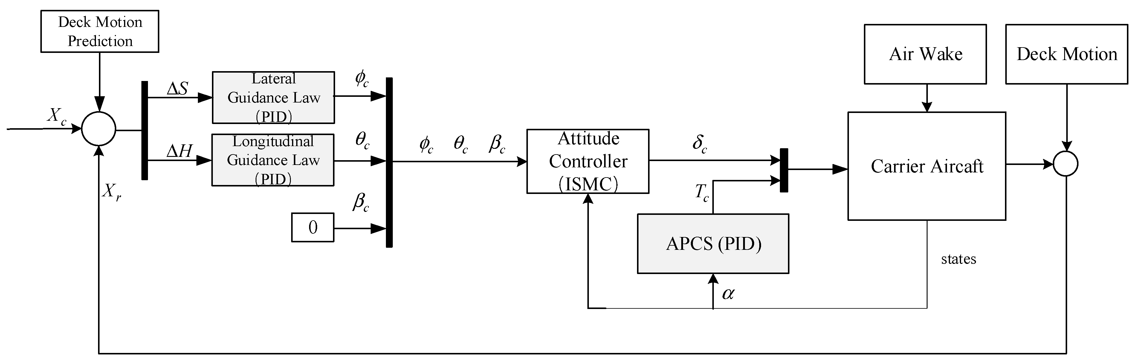
For the longitudinal control, the guidance law generates the pitch angle commands using the altitude tracking errors. At the same time, the automatic power compensation system (APCS) keeps the angle of attack at a steady state. Therefore, it is feasible to control the altitude by controlling the pitch angle. For the lateral control, the guidance law calculates the roll angle commands through the side distance tracking errors. This section introduces the automatic carrier landing control system with its guidance law designed using the PID method. The overall control structure of the ACLS is as follows (Figure 4).
In the ACLS, the APCS is designed as follows:
where , , , represent elevator deflection, normal load factor, thrust, and increments of the variables, respectively.
The longitudinal guidance law is designed using the PID method as follows:
with the height. The lateral PID guidance law is designed as follows:
with the side distance tracking errors. The controller parameters are designed in Table 3 as follows for the aircraft model used in this paper.
3. Optimal Preview Control-Based Guidance Law Considering Deck-Motion Compensation
In the landing control process, if the carrier aircraft only follows the glide path commands calculated from the current deck motion, a phase lag will show up in the command tracking. This is due to the influence of the deck motion. To solve this problem, this paper proposes a guidance law based on optimal preview control. The guidance law would combine the predicted deck motion with the dynamics of the carrier aircraft to effectively compensate for the phase lag, thereby improving the landing control accuracy. Since the longitudinal deck motion has a major influence on the landing accuracy of the carrier aircraft, the work of this paper is mainly focused on designing a longitudinal guidance law using the optimal preview control method.
3.1. Optimal Preview Control Method
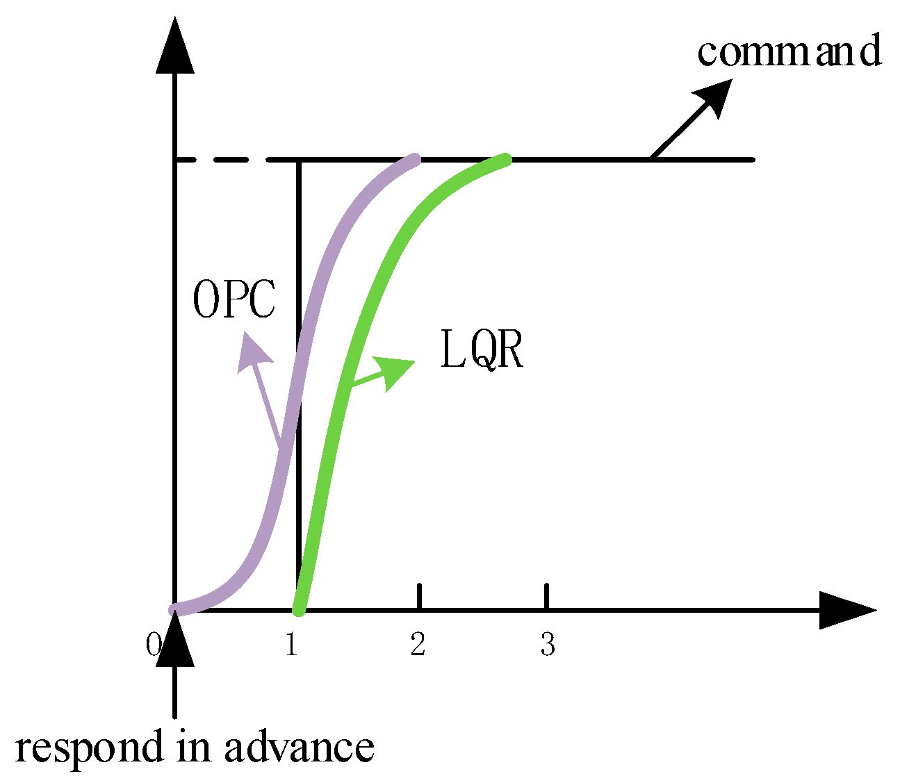
The optimal preview control solves the optimal control problem where the future control commands are known or predictable. For example, if it is known that there will be a step command after 1 s, traditional control methods (such as linear quadratic regulator, LQR) can only react to the command after 1 s, but the optimal preview control method can respond in advance by using the future command information, see Figure 5.
In general, the deck motion mainly consists of periodic components and random components. Due to the existence of the periodic component, the deck motion has good predictability. Correspondingly, the future glide path commands of the carrier aircraft are also predictable. Then, the optimal preview control method can be applied to realize the landing guidance of the carrier aircraft.
In this section, the discrete optimal preview control method is introduced. Consider a generalized system as follows:
where is the state vector, is the control vector, is the output vector.
Suppose that the reference command of the output is , the tracking error can be described as . Defining the incremental variables as , then the augmented model can be derived from Equation (22):
where , , , , , .
For the system described by Equation (23), it is assumed that the next steps of commands can be foreseen at every sampling time; then, the cost function of the following form can be constructed:
Similar to the idea of the LQR method, the optimal preview control also calculates the control inputs by minimizing the cost function shown in Equation (24). For conciseness, a detailed derivation process of OPC is not given in this paper; the readers are referred to Ref. [9] if interested. Finally, the control law is obtained as follows:
In Equation (25), the state feedback gain and the feedforward gain can be calculated as follows:
where , is the solution of the following Riccati equation:
3.2. Optimal Preview Control-Based Guidance Law Design through Low-Order Equivalent Fitting
In the existing literature, the optimal preview control is used to design an automatic carrier landing system in an integrated guidance and control (IGC) framework, and carrier motion can be successfully compensated in this way. In this work, a full-state linearized model of the aircraft is required; therefore, the control performance of this method may degrade when the linear model mismatches. In this paper, the optimal preview control is only applied to design the outer-loop guidance law, and a nonlinear control method, which depends less on aircraft model information, is adopted to design the attitude controller.
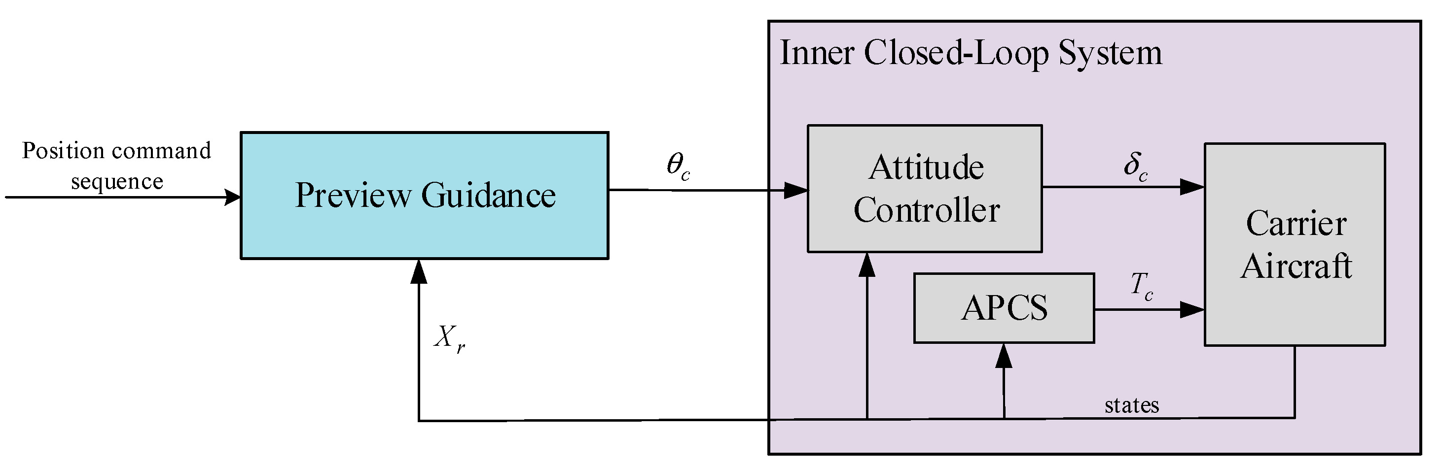
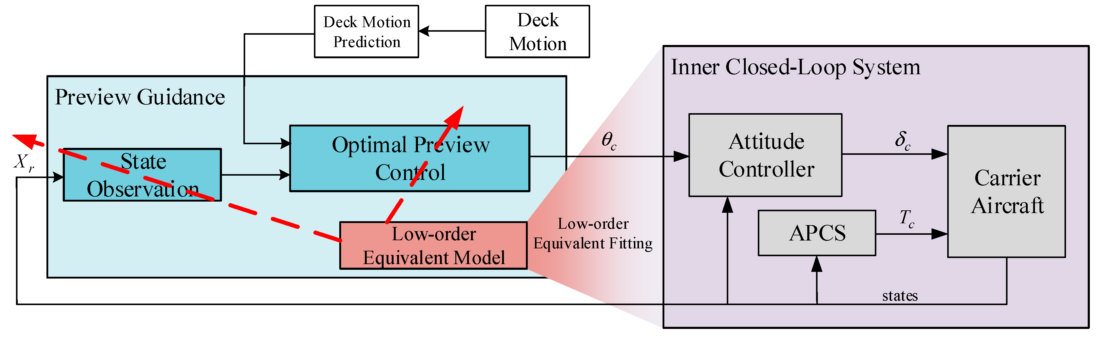
The control framework for the landing control system is illustrated in Figure 6. For the preview guidance law design, the controlled plant is the inner closed-loop system including an attitude controller and the APCS. As shown in Figure 6, the design of the preview guidance law also requires the linear model of the controlled plant. In this model, the attitude command becomes the input, and the position becomes the output. Fortunately, an advanced adaptive attitude controller is designed in the inner loop; the dynamics of the inner closed-loop system will be less affected by the aircraft dynamics since the inner controller are supposed to be of high performance. In this way, the model dependence of the ACLS proposed in this paper is reduced, which mainly occurs in the inner loop.
For the longitudinal control of the carrier landing, the input and output of the inner closed-loop system is the pitch angle command and the altitude, respectively. Although an APCS is included in this control system, the angle of attack will also change when the pitch angle rapidly changes. Therefore, cannot be simply used as the linear model for the outer loop in the design of the guidance law. On the other hand, directly linearizing the inner closed-loop system will result in a very complex high-order model. The high-order model is not beneficial to designing the guidance law, and it is also difficult to accurately obtain in practice. Therefore, in order to obtain a more accurate linear model for designing the preview guidance law, this paper introduces the low-order equivalent fitting approach.
Take the longitudinal guidance law design as an example. Firstly, trim the model of the carrier aircraft at the desired altitude and speed. Then, the frequency characteristics of the inner closed-loop system with pitch angle command as inputs and altitude as outputs is obtained by frequency sweeping. In this paper, a number of points are selected in the given frequency range:. Since the bandwidth of the pitch angle command is not higher than 10 rad/s, only the frequency characteristics below 10 rad/s need to be considered.
After obtaining the frequency-domain input/output data, take as the cost function to perform low-order equivalent fitting. In the abovementioned cost function, and are the responding amplitudes of the low-order system and the high-order system, respectively, and are the responding phases of the low-order system and the high-order system, respectively, and is the weight of the phase fitting errors.
In the low-order equivalent fitting procedure, the order of the low-order equivalent system should be as low as possible if the model accuracy is already ensured to be acceptable. Simulation experiments show that the fourth-order model is already able to accurately fit the inner closed-loop system. Therefore, a fourth-order transfer function is selected as the low-order equivalent model in this paper. To solve the fitting problem, the sequential quadratic programming (SQP) optimization algorithm is used to optimize the polynomial coefficients of the transfer function model.
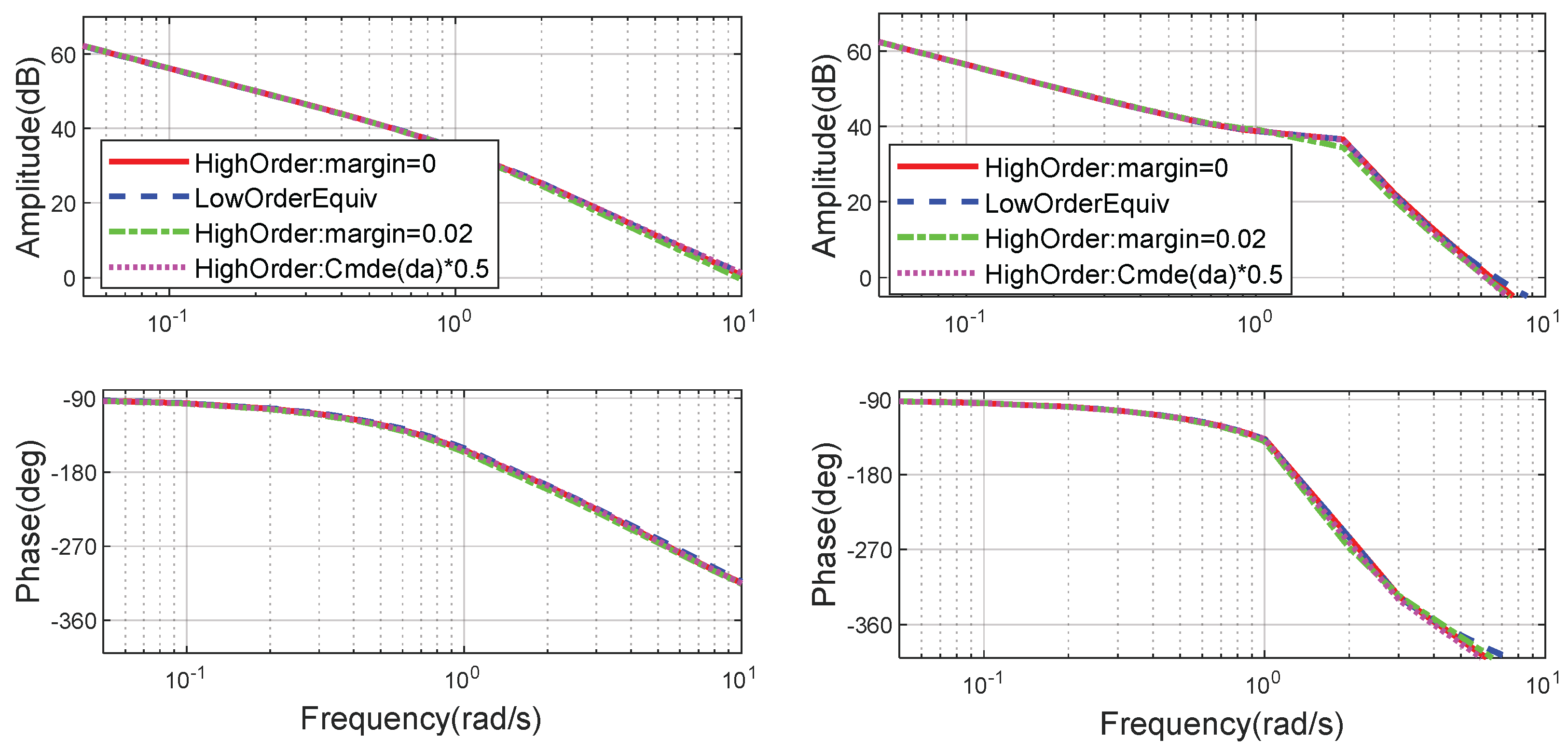
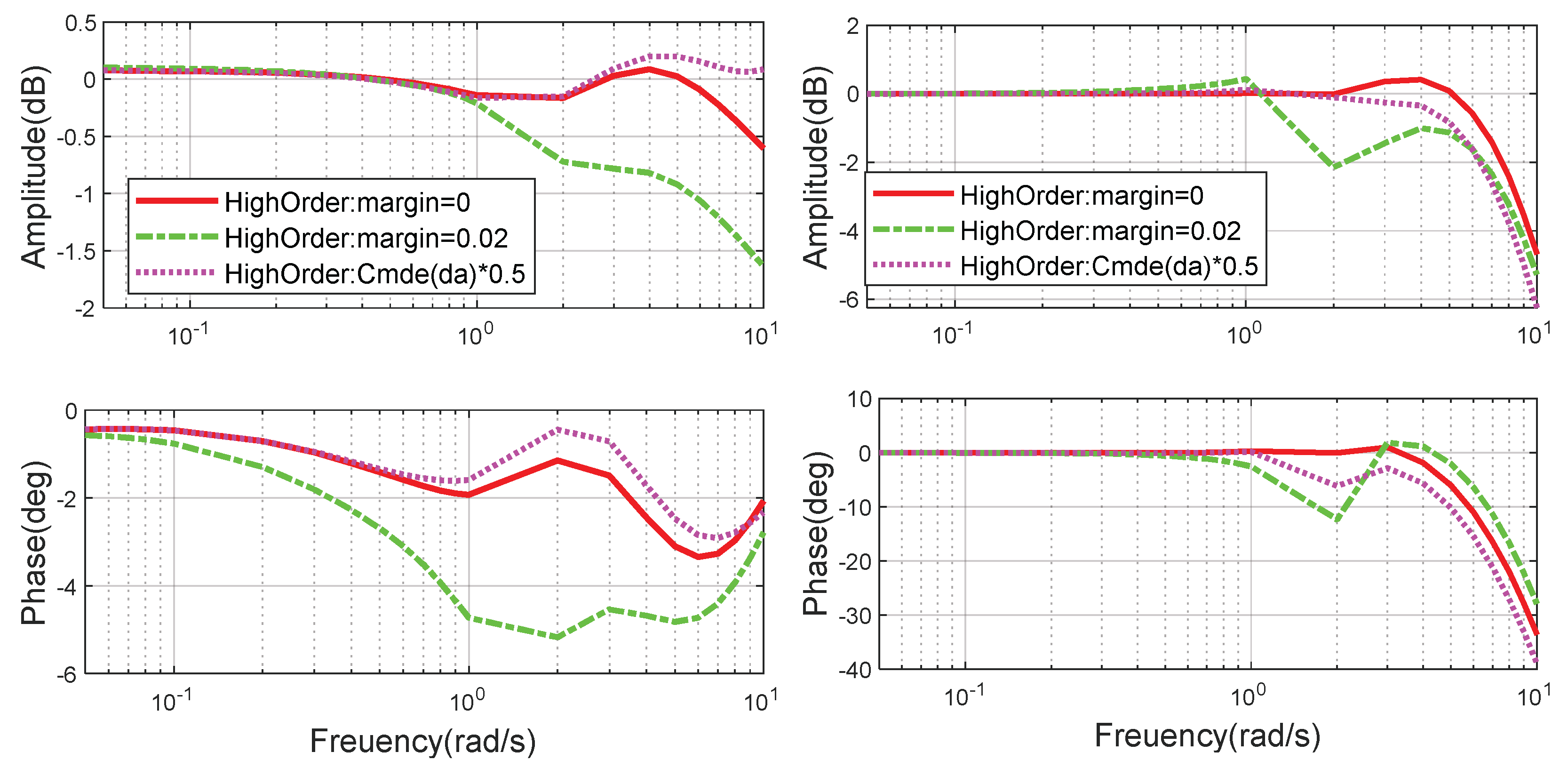
The low-order fitting results are given in Figure 7. Furthermore, to demonstrate that the dynamics of the inner closed-loop system are less affected by the dynamics of the carrier aircraft, a Bode diagram of the inner closed-loop system is given for the cases in which the aircraft suffers from center-of-gravity shift and elevator control efficiency reduction; see Figure 8. For comparison purposes, the PID control law is used to design the attitude controller for the aircraft according to Ref. [2], and the comparison results are given in Figure 7 and Figure 8. In the model uncertainty simulation scenarios, the center of gravity is moved forward by 2% and the elevator control efficiency is reduced by 50%. In the legends of Figure 7 and Figure 8, ‘margin = 0.02′ denotes that the center of gravity is shifted by 2%, and ‘Cmde(da)*0.5′ means the control efficiency of elevator and aileron is reduced by 50%.
As can be seen from the fitting results, the low-order equivalent system not only accurately fits the closed-loop system well when the aircraft is in the nominal state, but also achieves good fitting performance when the center of gravity suddenly changes and the control efficiency dramatically decreases. It indicates that the controller of the inner loop has a highly robust and fault-accommodation performance considering the aircraft dynamic changes, which ensures that the low-order equivalent fitting from the pitch commands to altitude is feasible. According to the plots in Figure 8, compared to the traditional PID controller, the ISC controller can ensure that the closed-loop system suffers less from model uncertainties or faults. In summary, the ISC controller is helpful in providing a more accurate model for designing the outer-loop guidance law.
3.3. State Observer Design for Low-Order Equivalent System
When designing the guidance law using OPC, the original inner closed-loop system is represented by a low-order equivalent linear system, and the state variables of this low-order system have no actual physical meaning except the first augmented state variable; i.e., the altitude tracking error. Therefore, these variables in the low-order system cannot be directly measured. In order to obtain the state variables in a real-time way for the OPC-based guidance law, it is necessary to design a state observer to observe the intermediate state variables. The overall control structure of the preview guidance law is illustrated in Figure 9.
Firstly, the inner closed-loop system is fitted into a low-order equivalent model. Then, the state observer and the optimal preview control law are designed using the low-order equivalent linear model. Finally, with the observed states and the predicted future deck motion sequence, the attitude commands can be calculated for the inner loop attitude controller.
The LQR method is used to design the Luenberger state observer in this paper:
where , with a Riccati equation:
3.4. ACLS Based on Deck Motion Prediction, Preview Guidance, and ISMC-Based Attitude Controller
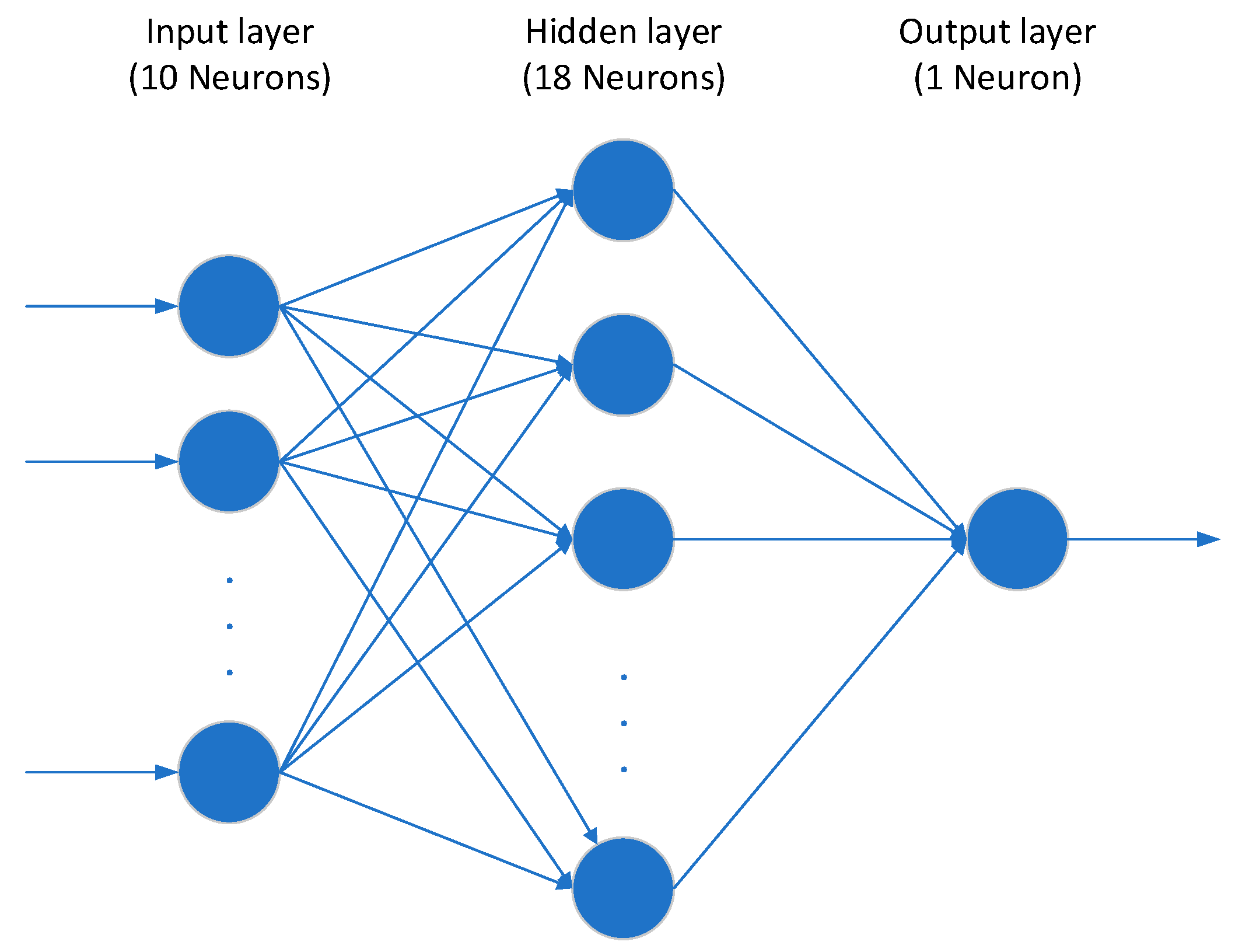
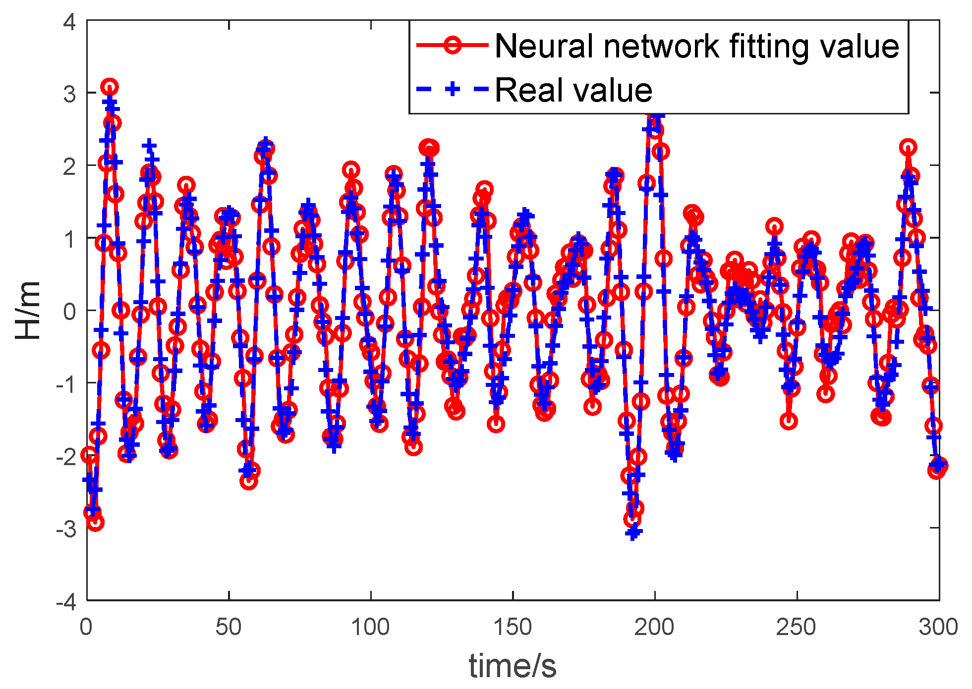
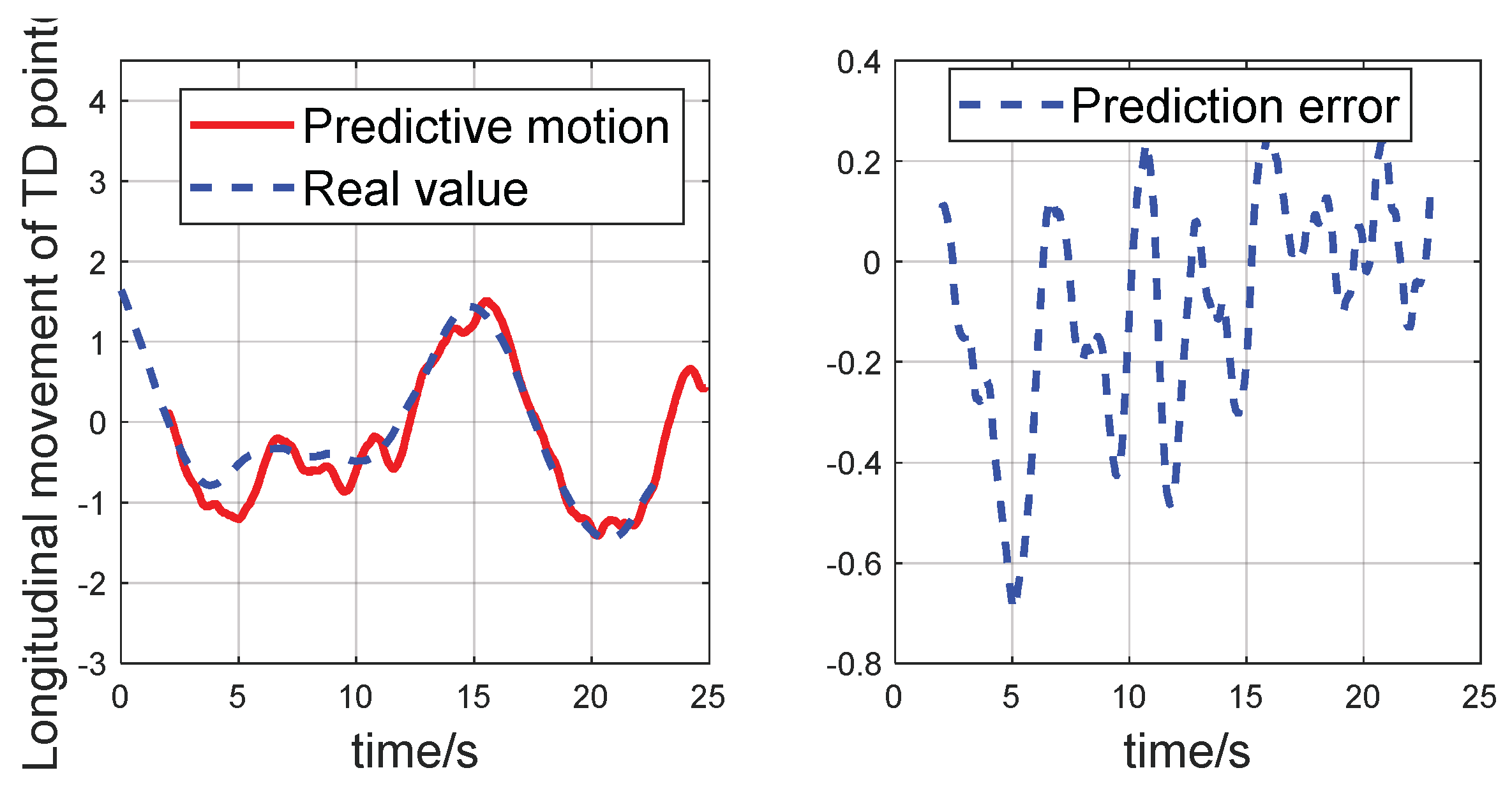
In the OPC-based guidance law, the future deck motion is required. Therefore, it is necessary to predict the future movements of the deck. In this paper, the neural network method [36] is used to build a prediction model for the deck motion. Firstly, collect the movements of the carrier for a certain period. Then, train the neural networks with these data in an offline manner. Finally, for real-time application, the trained neural network model is used to predict the deck motion in the landing process. The structure of the neural network model is shown in Figure 10. We choose a neural network with only one hidden layer because the prediction method is found to be insensitive to the number of layers. Specifically, there are 10 neurons in the input layer, 18 neurons in the hidden layer, and one neuron in the output layer; 10 neurons are chosen for the input layer because the period of the carrier aircraft is about 10 s, and the input state should preferably cover the past 10 s. Considering the amount of data and the difficulty of training, this paper selects a total of 10 ship motion states every 1 s as the input; that is, the number of neurons in the input layer is 10. One neuron of the output layer represents the ship movement after 2 s. The 18 neurons selected in the hidden layer are tuned according to the experience, which is the approximation of precision and performance.
Figure 11 and Figure 12 show the fitting results of the neural networks and the prediction results of the deck motion, respectively.
Finally, by synthesizing the works from section III.B, IV.B, and IV.C, a novel ACLS is developed based on the preview guidance law and the incremental sliding mode attitude controller; see Figure 13.
Considering that the lateral motion of the deck has less influence on the landing accuracy of carrier aircraft compared to the longitudinal deck motion, the PID guidance law is adopted for the lateral operations in this paper.
4. Simulation Results and Analysis
In this section, three simulation experiments were performed to demonstrate the effectiveness of the ACLS, which consisted of an optimal preview control-based guidance law and an ISMC-based attitude controller; this synthesized landing control approach is called OPC-ISMC in the remainder of this paper.
Firstly, the results of OPC and PID guidance law are used to track sine wave type altitude commands in order to verify the effect of the OPC guidance law on compensation of the deck motion. Secondly, the automatic landing control performances of three landing control approaches, i.e., OPC-ISMC, PID-ISMC, and an integrated guidance and control (IGC) system based on OPC and the full-state linear model (OPC-IGC), as in the existing literature [8,9], are compared under complex sea conditions. The purpose is to show that the OPC-ISMC can better achieve disturbance rejection control, and can effectively compensate for the deck motion. Finally, the Monte Carlo simulation of automatic landing processes using these three kinds of ACLS is performed to further verify that the OPC-ISMC-type ACLS designed in this paper can result in higher landing accuracy and stronger robustness.
The dynamics of an ESSEX class carrier are employed throughout this paper, and the power spectrum of this carrier with sea state level 4 is modeled and used in the simulations. Detailed data for air wake can be found in Ref. [32], and the data for the deck motion model can be found in Ref. [32].
4.1. Comparison of OPC and PID Guidance Laws
- (1)
- Time domain comparison
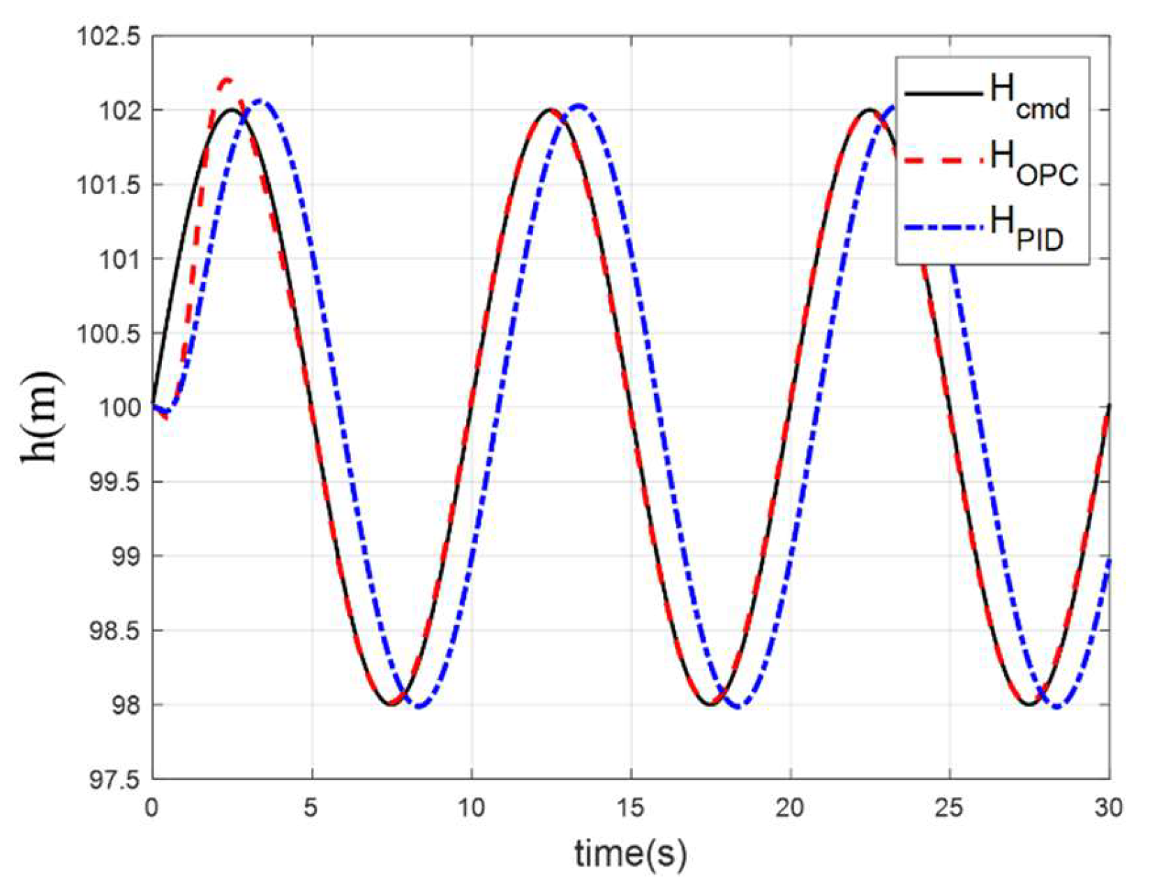
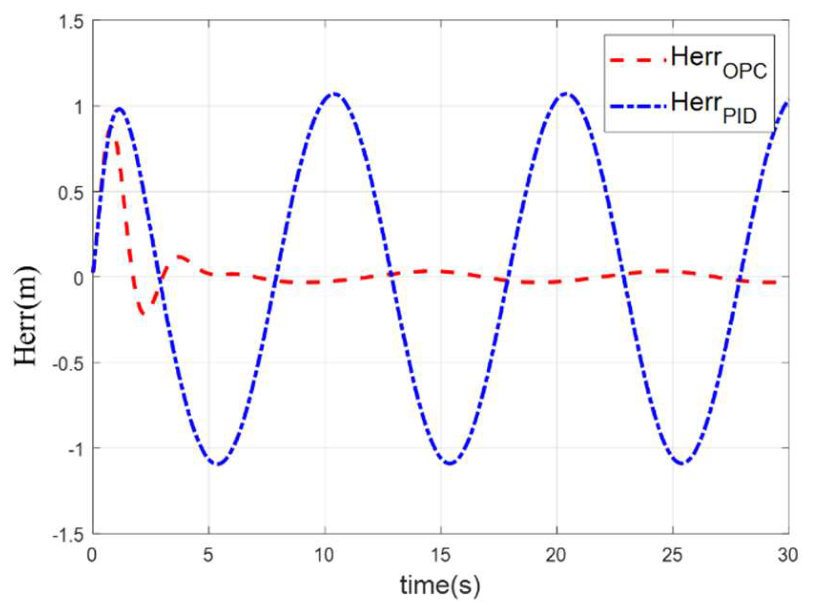
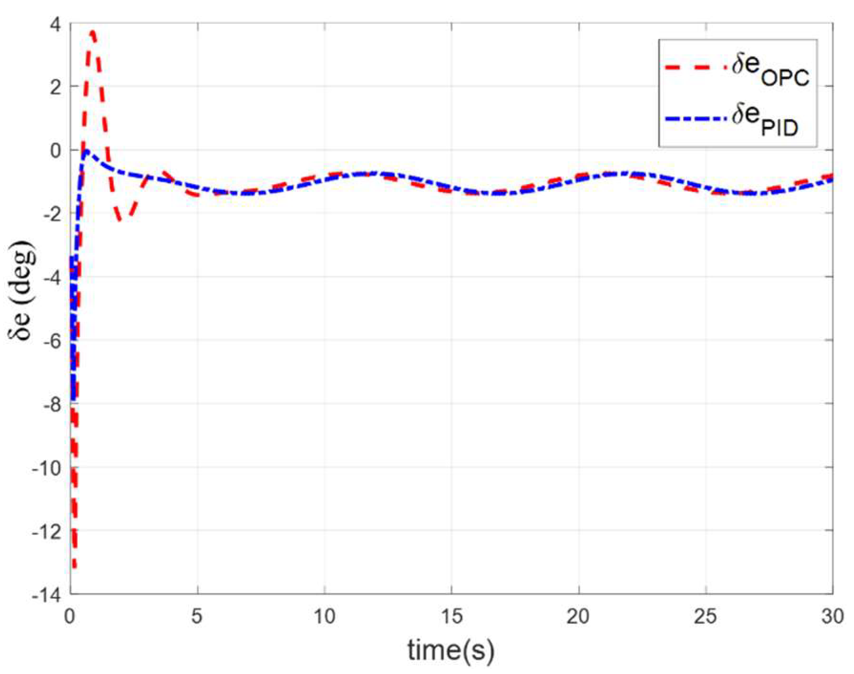
To simulate the motion of the aircraft carrier, a sine wave type altitude command with a period of 10 s and an amplitude of 2 m is given, and it is assumed that the command in the future 2 s can be accurately predicted. For the landing control system, the ISMC attitude controller is used in the inner loop, and the OPC and PID are separately used as guidance laws to track the altitude commands. The results are given in Figure 14, Figure 15, Figure 16 and Figure 17.
It can be seen from Figure 14 and Figure 15 that when the PID is used as the guidance law, the altitude always lags behind the command for about 1 s, and the maximum tracking error is 1.04 m after reaching the steady state. When the OPC is used as the guidance law, not only does the tracking time delay disappear, but the amplitude of the maximum tracking error is also reduced to 0.04 m when reaching the steady state.
As shown in Figure 16 and Figure 17, when the OPC is used, large pitch angle commands and elevator commands will be generated at the beginning, and the command phase of pitch commands for the OPC is always ahead of those for the PID. This is because the OPC makes full use of the known future command information, and makes the aircraft respond in advance, so it can greatly reduce the tracking delay, and thus improve the control accuracy.
- (2)
- Frequency domain comparison
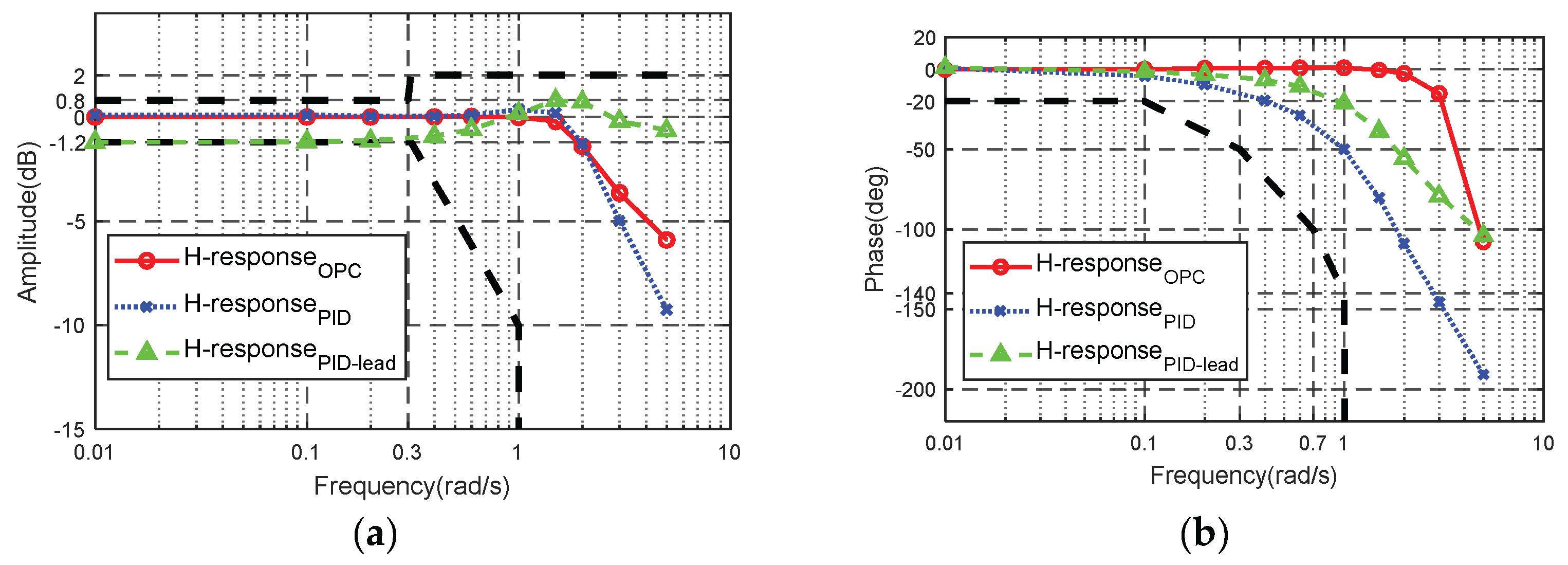
To further compare the OPC-based guidance law with the PID guidance law, a bode diagram of the closed-loop system in terms of altitude tracking is given below. Meanwhile, the Navy specification guideline requirements [31] of the closed-loop system in terms of altitude tracking are given in the plots as references; see Figure 18.
In practical applications, the guidance law for ACLSs often consists of a Deck Motion Compensation (DMC) filter to compensate for the phase lag caused by the deck motion [2,23]. In this paper, a DMC filter is also designed together with the PID guidance law, and this is named PID-lead. The DMC filter takes the form from Ref. [23]:
where the extra term is to suppress the high-frequency noise. The corresponding parameters are in Table 4 as follows:
Figure 18 shows that the phase lag of the system using the OPC guidance law is much smaller than using the PID guidance law. In addition, it also shows that compared to the PID-lead compensator, the OPC guidance law performs better in compensating for the phase lag and keeping the amplitude constant.
Another way to compensate for the phase lag is to directly add the future deck motion to the altitude command. However, it is hard to determine the specific leading time of the deck motion. If the leading time is too small, the system will still lag. If the leading time is too large, it may even lead to a phase leading phenomenon, which will also result in large tracking errors.
4.2. Comparison of Different ACLSs under Complex Sea Conditions
In this section, the atmospheric environment on the sea, i.e., air wake, and the deck motion are considered. Specifically, the deck motion is modeled using the power spectral density function method. Three ACLSs are simulated for comparison purpose: OPC-ISMC, PID-ISMC, and OPC-IGC.
In the simulation, the speed of the carrier is set as 25 kn (12.86 m/s), and the deck angle is set as—8°. The forward direction of the carrier is selected as the axis of the inertial frame. The initial position of the carrier aircraft is set at m in the inertial frame, the initial velocity is 66 m /s, and the initial pitch angle is 3.5°.
- (1)
- Normal case
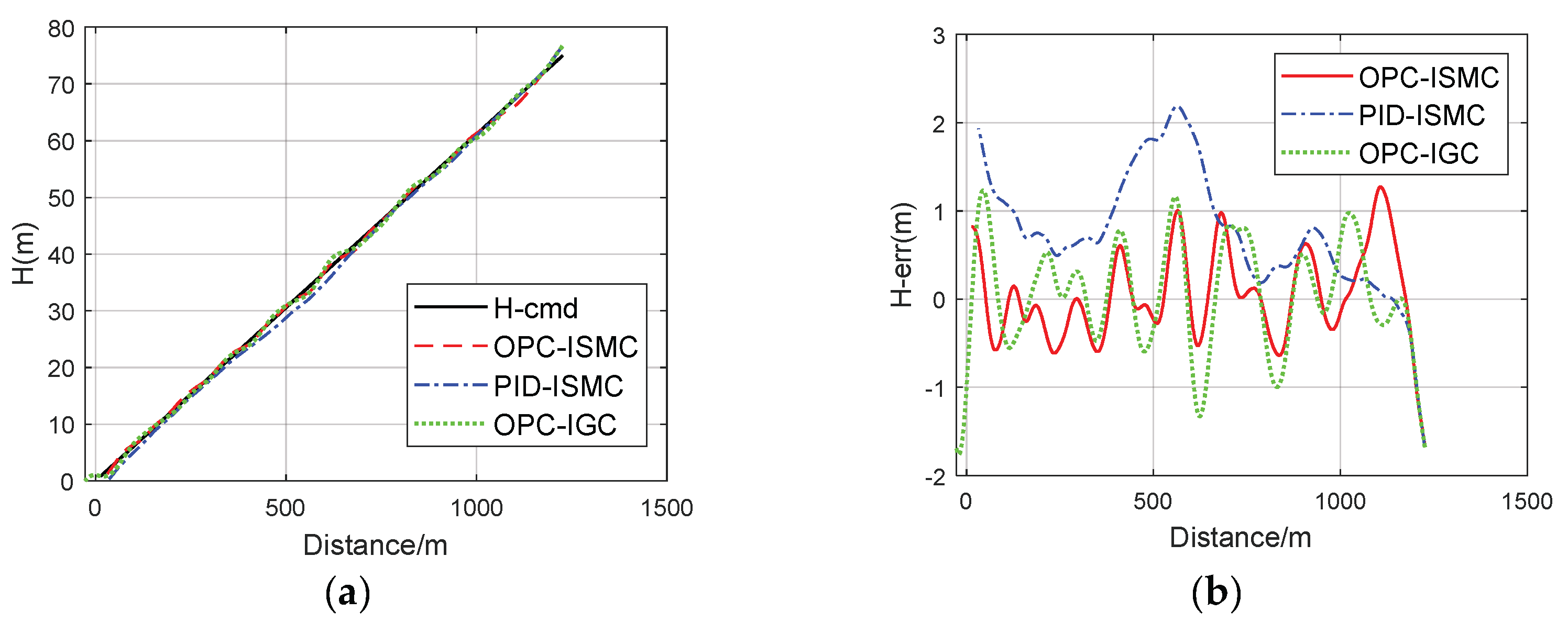
As can be seen from Figure 19, in the normal case, the altitude tracking errors of the carrier aircraft using OPC-ISMC and OPC-IGC are much smaller than those using PID-ISMC. This indicates that PID-ISMC is significantly influenced by the deck motion, while the other two methods can partly compensate for the deck motion influence.
- (2)
- Aircraft model deviation case (center of gravity shift forward 2% before landing)
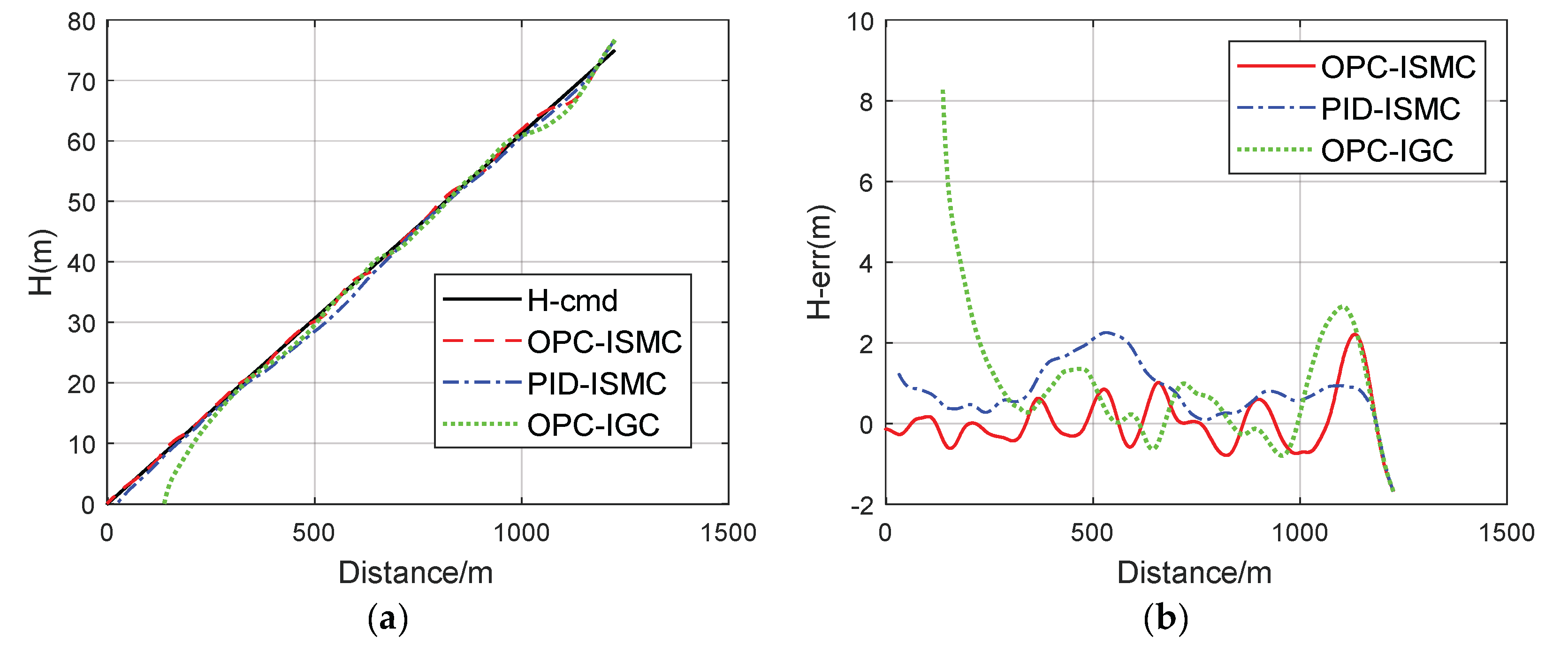
As can be seen from Figure 20, when the model deviates, the altitude tracking performances of OPC-ISMC and PID-ISMC have almost no changes due to the strong adaptability of the ISMC attitude controller. For the OPC-IGC ACLS, the altitude tracking error significantly increases (up to 8 m) when the center of gravity is shifted. This is due to the fact that the OPC-IGC depends on the highly accurate linear model.
- (3)
- Sudden disturbance case (center of gravity suddenly moves forward by 2% at 16 s)
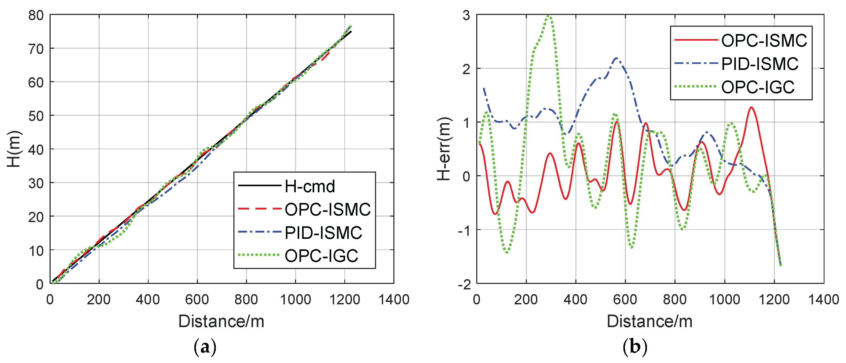
As can be seen from Figure 21, when PID-ISMC and OPC-ISMC are used, the sudden disturbance at 16 s has little influence on the control accuracy of altitude. This is due to the strong disturbance rejection and fault tolerance capability of the ISMC. However, the OPC-IGC guidance control system is incapable of quickly recovering from the disturbance, and this results in large altitude tracking errors.
4.3. Monte Carlo Simulation Tests of Different ACLSs
This section outlines the Monte Carlo tests carried out on three ACLSs, namely OPC-ISMC, PID-PID, and PID-PID-Pred; where PID-PID-Pred means an integration of the PID guidance law, the PID attitude controller, and the deck motion prediction unit. Note that PID-PID-Pred is the classical guidance and control approach in designing a ACLS. In practice, the deck motion and sea surface wind vary with time, and the deck may be pitching up or pitching down when the aircraft is beginning to land. Therefore, statistical results are given in this section to validate the proposed method. A total of 100 carrier landing simulation experiments were carried out with different settings of the initial carrier deck states. In order to verify the adaptation capability of the ACLSs to model uncertainties, in addition to the nominal case, the case of a center of gravity change and the case of a left elevator being stuck were also chosen as scenarios. In the work of this section, medium sea conditions were chosen for simulation.
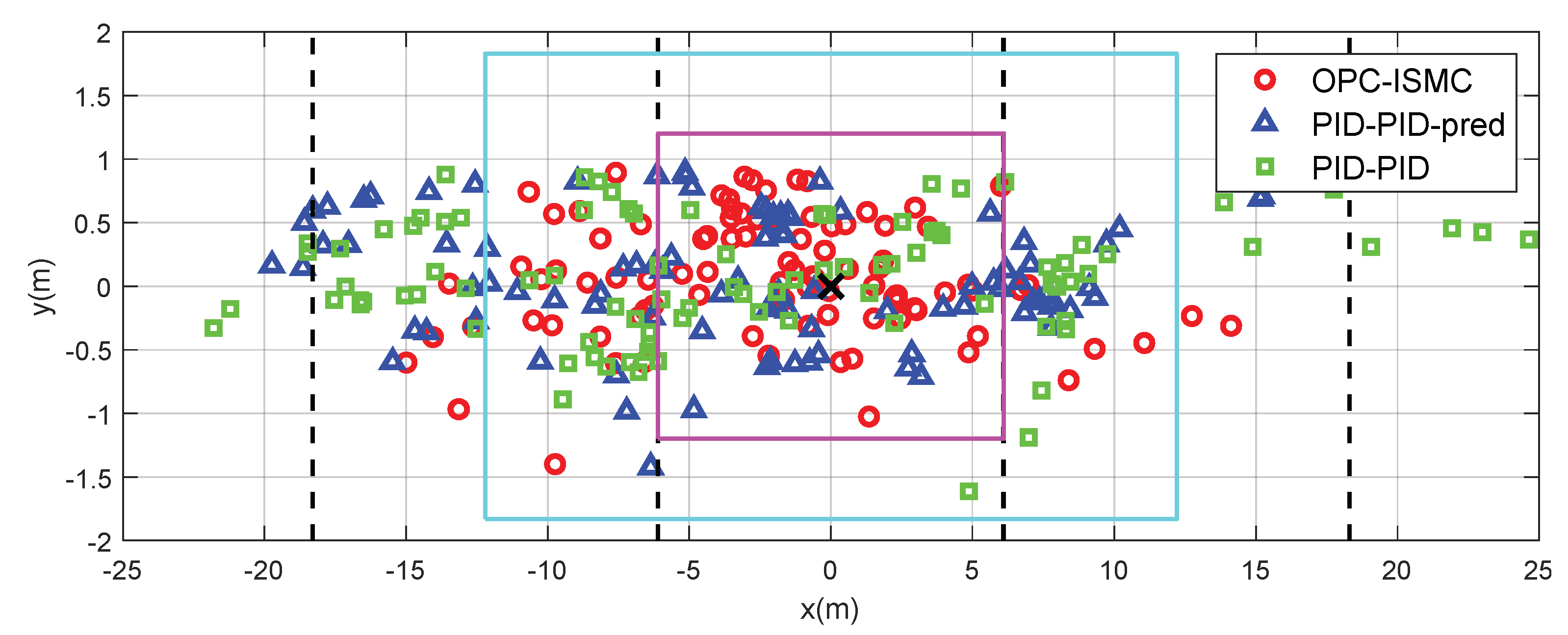
Before the simulations, the successful landing rate and ideal landing rate needed to be defined. The successful landing rate and the ideal landing rate refer to the percentage of successful landings of the carrier aircraft in the allowable landing area and the ideal landing area, respectively. As shown in Figure 22, the light blue square is the allowable landing area, and the pink square is the ideal landing area. Here, the touch down point reflects the precision of the landing end. The landing deviation is the most important factor that researchers/industries are concerned with, and it has the greatest impact on landing.
- (1)
- Case 1: nominal case (without center of gravity moved forward and the left elevator stuck)
- (2)
- Case 2: center of gravity is moved forward by 2%
- (3)
- Case 3: the left elevator is stuck at −15°
According to the results in Table 5, Table 6 and Table 7 and Figure 22, Figure 23 and Figure 24, the Monte Carlo test results show that the OPC-ISMC-based automatic landing system can guarantee that the successful landing rate is over 90% in medium sea conditions for cases 1, 2, and 3. Furthermore, when using OPC-ISMC, the standard deviation of longitudinal landing errors, which is the distance between the touchdown point and the ideal landing point, is also the smallest.
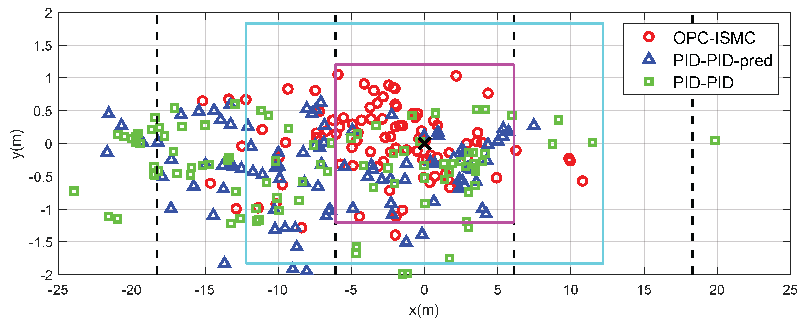
In the case of the left elevator being stuck, the PID-PID-based ACLS will lead to the phenomenon where the carrier aircraft deviates to the left of the touch down points in a statistical sense. While the touch down point results from OPC-ISMC are still symmetrically distributed in a statistical sense. This reflects that the OPC-ISMC-based ACLS has strong anti-disturbance and fault-tolerant capabilities.
5. Conclusions
This paper is focused on designing an advanced automatic carrier landing system (ACLS) to improve the landing performance of carrier aircraft in complex conditions, such as air wake and deck motion. The main results are concluded as follows.
- (1)
- A novel ACLS synthesizing a preview control-based guidance law and an incremental type nonlinear adaptive attitude controller is proposed in this paper. The overall control system design scheme, including designing a nonlinear attitude controller, a low-order equivalent fitting procedure, and an optimal preview control (OPC)-based guidance law, is developed.
- (2)
- In order to improve the disturbance rejection ability of the attitude loop, an attitude controller is designed using the finite-time incremental sliding mode control approach after reformulating a second-order incremental aircraft model. To overcome the influence of deck motion, an optimal preview control is used to design an outer-loop guidance law. Since the optimal preview control method cannot be directly applied to design the outer-loop guidance law, this paper proposes a design method of the optimal preview-based guidance law through low-order equivalent fitting of inner closed-loop system and state estimation of the low-order equivalent system model.
- (3)
- Simulation results show that the OPC-ISMC-based ACLS developed in this paper can effectively improve the landing accuracy and successful landing rates under aircraft model uncertainties and complex sea conditions. Compared with the classical PID guidance law, it can more effectively compensate for the influence of the carrier motion. Compared with the integrated guidance and control (IGC) system based on OPC and a full-state linear aircraft model, it has stronger adaptive ability and disturbance rejection capability due to the high performance of the inner attitude loop.
Author Contributions
Conceptualization, L.S.; Methodology, B.J. and X.L.; Software, J.J.; Validation, X.L.; Formal analysis, B.J. and S.X.; Investigation, L.S., S.X. and W.T.; Resources, W.T.; Data curation, X.L., S.X. and J.J.; Writing—original draft, B.J.; Supervision, L.S. and W.T.; Funding acquisition, L.S. and W.T. All authors have read and agreed to the published version of the manuscript.
Funding
This study was co-supported by the Aeronautical Science Foundation of China (No. 20185702003) and the Fundamental Research Funds for the Central Universities of China (No. YWF-21-BJ-J-809).
Conflicts of Interest
The authors declare no conflict of interest.
References
- Dong, R.; Shao, X.; Wang, L.; Zhao, G.; Zhou, X. Efficient Linear Modeling Method of Carrier Landing Flight Dynamics. J. Aircr. 2021, 58, 1179–1186. [Google Scholar] [CrossRef]
- Urnes, J.M.; Hess, R.K. Development of the F/A-18A Automatic Carrier Landing System. J. Guid. Control Dyn. 1985, 8, 289–295. [Google Scholar] [CrossRef]
- Li, J.; Duan, H. Simplified Brain Storm Optimization Approach to Control Parameter Optimization in F/A-18 Automatic Carrier Landing System. Aerosp. Sci. Technol. 2015, 42, 187–195. [Google Scholar] [CrossRef]
- Sánchez-Sánchez, C.; Izzo, D. Real-time optimal control via deep neural networks: Study on landing problems. J. Guid. Control Dyn. 2018, 41, 1122–1135. [Google Scholar] [CrossRef] [Green Version]
- Alvarez, D.; Lu, B. Piloted simulation study comparing classical, H-infinity, and linear parameter-varying control methods. J. Guid. Control Dyn. 2011, 34, 164–176. [Google Scholar] [CrossRef]
- Sheng, L.; Zhang, W.; Gao, M. Mixed H-2/H-infinity control of time-varying stochastic discrete-time systems under uniform detectability. IET Control Theory Appl. 2014, 8, 1866–1874. [Google Scholar] [CrossRef]
- Misra, G.; Bai, X.L. Output-Feedback Stochastic Model Predictive Control for Glideslope Tracking during Aircraft Carrier Landing. J. Guid. Control Dyn. 2019, 42, 2098–2105. [Google Scholar] [CrossRef]
- Zhen, Z.Y.; Jiang, S.Y.; Jiang, J. Preview Control and Particle Filtering for Automatic Carrier Landing. IEEE Trans. Aerosp. Electron. Syst. 2018, 54, 2662–2674. [Google Scholar] [CrossRef]
- Zhen, Z.Y.; Jiang, S.Y.; Ma, K. Automatic Carrier Landing Control for Unmanned Aerial Vehicles Based on Preview Control and Particle Filtering. Aerosp. Sci. Technol. 2018, 81, 99–107. [Google Scholar] [CrossRef]
- Rodriguez-Ramos, A.; Sampedro, C.; Bavle, H.; De La Puente, P.; Campoy, P. A deep reinforcement learning strategy for UAV autonomous landing on a moving platform. J. Intell. Robot. Syst. 2019, 93, 351–366. [Google Scholar] [CrossRef]
- Che-Cheng, C.; Tsai, J.; Peng-Chen, L.; Lai, C.A. Accuracy Improvement of Autonomous Straight Take-off, Flying Forward and Landing of a Drone with Deep Reinforcement Learning. Int. J. Comput. Intell. Syst. 2020, 13, 914. [Google Scholar] [CrossRef]
- Zhang, S.; Li, Y.; Dong, Q. Autonomous navigation of UAV in multi-obstacle environments based on a Deep Reinforcement Learning approach. Appl. Soft Comput. 2022, 115, 108194. [Google Scholar] [CrossRef]
- Zhen, Z.Y.; Yu, C.J.; Jiang, S.Y.; Jiang, J. Adaptive super-twisting control for automatic carrier landing of aircraft. IEEE Trans. Aerosp. Electron. Syst. 2019, 56, 984–997. [Google Scholar] [CrossRef]
- Zhen, Z.Y.; Tao, G.; Yu, C.J.; Xue, Y.X. A multivariable adaptive control scheme for automatic carrier landing of UAV. Aerosp. Sci. Technol. 2019, 92, 714–721. [Google Scholar] [CrossRef]
- Yue, Y.; Wang, H.L.; Li, N.; Su, Z.K. Automatic carrier landing system based on active disturbance rejection control with a novel parameters optimization. Aerosp. Sci. Technol. 2017, 69, 149–160. [Google Scholar] [CrossRef]
- Guan, Z.Y.; Liu, H.; Zheng, Z.W.; Lungu, M.H. Fixed-time control for automatic carrier landing with disturbance. Aerosp. Sci. Technol. 2021, 108, 106403. [Google Scholar] [CrossRef]
- Guan, Z.Y.; Ma, Y.P. Moving Path following with Prescribed Performance and Its Application on Automatic Carrier Landing. IEEE Trans. Aerosp. Electron. Syst. 2020, 56, 2576–2590. [Google Scholar] [CrossRef]
- Guan, Z.Y.; Ma, Y.P.; Zheng, Z.W.; Guo, N. Prescribed performance control for automatic carrier landing with disturbance. Nonlinear Dyn. 2018, 94, 1335–1349. [Google Scholar] [CrossRef]
- Liu, Z.; Zhang, Y.; Liang, J.; Chen, H. Application of the Improved Incremental Nonlinear Dynamic Inversion in Fixed-Wing UAV Flight Tests. J. Aerosp. Eng. 2022, 35, 04022091. [Google Scholar] [CrossRef]
- Smeur, E.J.J.; Croon, G.D.; Chu, Q. Cascaded incremental nonlinear dynamic inversion for MAV disturbance rejection. Control Eng. Pract. 2018, 73, 79–90. [Google Scholar] [CrossRef] [Green Version]
- Wang, X.R.; Kampen, E.J.V.; Chu, Q.; Lu, P. Incremental Sliding-Mode Fault-Tolerant Flight Control. J. Guid. Control Dyn. 2019, 42, 244–259. [Google Scholar] [CrossRef]
- Ireland, M.L.; Flessa, T.; Thomson, D.; McGookin, E. Comparison of Nonlinear Dynamic Inversion and Inverse Simulation. J. Guid. Control Dyn. 2017, 40, 3307–3312. [Google Scholar] [CrossRef] [Green Version]
- Schust, A.P.; Young, P.N.; Simpson, W.R. Automatic Carrier Landing System (ACLS) Category III Certification Manual; AD-A118181; Defense Technical Information Center: Washington, DC, USA, 1982. [Google Scholar]
- Li, L.; Liao, F. Robust preview control for a class of uncertain discrete-time systems with time-varying delay. ISA Trans. 2018, 73, 11–21. [Google Scholar] [CrossRef] [PubMed]
- Li, D.M.; Zhou, D.; Hu, Z.K.; Hu, H.Z. Optimal preview control applied to terrain following flight. In Proceedings of the 40th IEEE Conference on Decision and Control, Orlando, FL, USA, 4–7 December 2001; IEEE: Piscataway, NJ, USA, 2001; pp. 211–216. [Google Scholar]
- McCabe, J.S.; DeMars, K.J. Anonymous feature-based terrain relative navigation. J. Guid. Control Dyn. 2020, 43, 410–421. [Google Scholar] [CrossRef]
- Barfield, A.F.; Hinchman, J.L. An Equivalent Model for UAV Automated Aerial Refueling Research. In AIAA Modeling and Simulation Technologies Conference and Exhibit; AIAA: Reston, VA, USA, 2005; pp. 1–7. [Google Scholar]
- Blake, W.; Okolo, W.; Dogan, A. Development of an Aerodynamics Model for a Delta-wing Equivalent Mode II (EQ-II) Aircraft. In AIAA Modeling and Simulation Technologies Conference and Exhibit; AIAA: Reston, VA, USA, 2005; pp. 1–28. [Google Scholar]
- Zheng, F.; Zhen, Z.; Gong, H. Observer-based backstepping longitudinal control for carrier-based UAV with actuator faults. J. Syst. Eng. Electron. 2017, 28, 322–377. [Google Scholar]
- Yue, L.; Liu, G.; Hong, G. Design and simulation of F/A-18A automation carrier landing guidance controller. In Proceedings of the AIAA Modeling and Simulation Technologies Conference, Washington, DC, USA, 13–17 June 2016; pp. 1–11. [Google Scholar]
- Guan, Z.; Liu, H.; Zheng, Z.; Ma, Y.; Zhu, T. Moving path following with integrated direct lift control for carrier landing. Aerosp. Sci. Technol. 2022, 120, 107247. [Google Scholar] [CrossRef]
- Chen, C.; Tan, W.Q.; Qu, X.J.; Li, H.X. A fuzzy human pilot model of longitudinal control for a carrier landing task. IEEE Trans. Aerosp. Electron. Syst. 2018, 54, 453–466. [Google Scholar] [CrossRef]
- Tan, W.; Efremov, A.V.; Qu, X. A criterion based on closed-loop pilot-aircraft systems for predicting flying qualities. Chin. J. Aeronaut. 2010, 23, 511–517. [Google Scholar]
- Yang, L.; Yang, J. Nonsingular fast terminal sliding-mode control for nonlinear dynamical systems. Int. J. Robust Nonlinear Control 2011, 21, 1865–1879. [Google Scholar] [CrossRef]
- Polyakov, A.; Fridman, L. Stability notions and Lyapunov functions for sliding mode control systems. J. Frankl. Inst. 2014, 351, 1831–1865. [Google Scholar] [CrossRef] [Green Version]
- Yin, J.; Zou, Z.; Xu, F. On-line prediction of ship roll motion during maneuvering using sequential learning RBF neural networks. Ocean. Eng. 2013, 61, 139–147. [Google Scholar] [CrossRef]
Figure 1.
Geometry of the tailless carrier aircraft.

Figure 2.
Carrier disturbance motion generator.

Figure 3.
ACLS control framework.

Figure 4.
Control structure of ACLS with PID-based guidance law and ISMC-based attitude controller.

Figure 5.
Comparison between OPC and LQR.

Figure 6.
Guidance law and the inner closed-loop system.

Figure 7.
Low-order equivalent fitting of the inner closed-loop system using ISC (left) and PID (right).
Figure 7.
Low-order equivalent fitting of the inner closed-loop system using ISC (left) and PID (right).

Figure 8.
Low-order equivalent fitting errors of using ISC (left) and PID (right).

Figure 9.
Control structure of the guidance law.

Figure 10.
Structure of the neural network model used to predict the deck motion.

Figure 11.
Fitting results of the neural networks in training.

Figure 12.
Prediction results of the neural networks in application.

Figure 13.
Novel ACLS based on OPC guidance law and ISC attitude controller.

Figure 14.
Tracking effects of OPC and PID.

Figure 15.
Tracking errors of OPC and PID.

Figure 16.
Pitch angle tracking performances.

Figure 17.
Comparison of elevator deflections.

Figure 18.
Amplitude-frequency and phase-frequency characteristic of height closed-loop system. (a) Amplitude-frequency characteristic. (b) Phase-frequency characteristic.
Figure 18.
Amplitude-frequency and phase-frequency characteristic of height closed-loop system. (a) Amplitude-frequency characteristic. (b) Phase-frequency characteristic.

Figure 19.
Comparison of glide path tracking responses for different ACLSs in the normal case. (a) Height variations. (b) Altitude tracking errors.
Figure 19.
Comparison of glide path tracking responses for different ACLSs in the normal case. (a) Height variations. (b) Altitude tracking errors.

Figure 20.
Comparison of glide path tracking responses for different ACLSs in the case of model deviation (C.G. shift). (a) Height variations. (b) Altitude tracking errors.
Figure 20.
Comparison of glide path tracking responses for different ACLSs in the case of model deviation (C.G. shift). (a) Height variations. (b) Altitude tracking errors.

Figure 21.
Comparison of glide path tracking responses of different ACLSs in the case of sudden disturbances. (a) Height variations. (b) Altitude tracking errors.
Figure 21.
Comparison of glide path tracking responses of different ACLSs in the case of sudden disturbances. (a) Height variations. (b) Altitude tracking errors.

Figure 22.
Touch down point distribution using three ACLSs under nominal case.

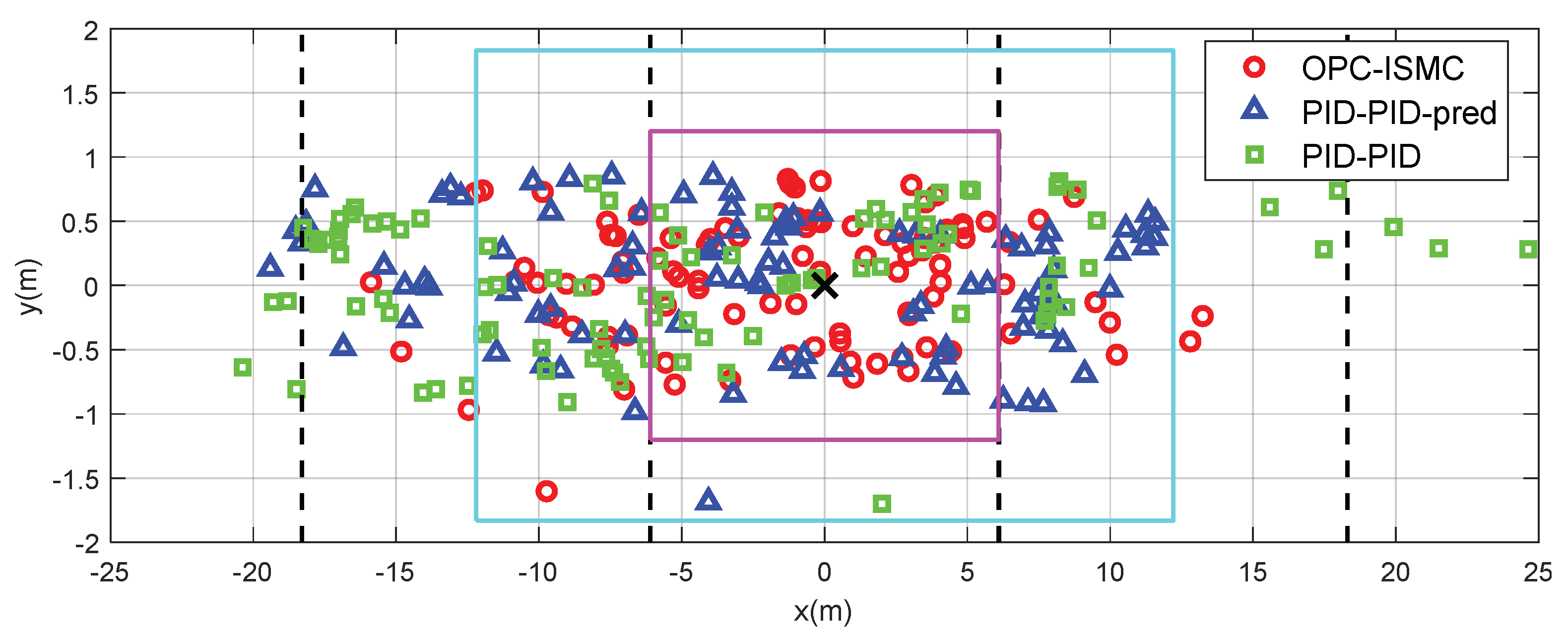
Figure 23.
Touch down points distribution of three ACLSs under the c.g. change case.

Figure 24.
Touch down point distribution of three ACLSs under the elevator stuck case.


Table 1.
Parameters of actuator and engine models.
| Actuators | |||||
|---|---|---|---|---|---|
| Symbol | Model | Natural Frequency (rad/s) | Damping Ratio | Amplitude Limit (deg) | Rate Limit (deg/s) |
| Second order | 50 | 0.8 | [−30, 30] | [−90, 90] | |
| Second order | 50 | 0.8 | [−45, 45] | [−90, 90] | |
| Second order | 50 | 0.8 | [0, 60] | [−90, 90] | |
| Engine | |||||
| Model | Frequency (rad/s) | Thrust limit (N) | Rate limit (N/s) | ||
| First order | 2.4 | [4448, 44,480] | [−6450, 8363] | ||
Table 2.
Transfer Function between the Carrier Motion and White Noise.
Table 3.
Parameters of the PID guidance law and APCS.
| Parameter | ||||||||||
|---|---|---|---|---|---|---|---|---|---|---|
| Value | 2.9 × 10⁶ | 2.9 × 10⁴ | 3 × 10⁴ | −1 × 10⁵ | 1.8 × 10⁻⁴ | 3 × 10⁻³ | 1.2 × 10⁻⁴ | 3.5 × 10⁻² | 1.7 × 10⁻³ | 0.1 |
Table 4.
Parameters of the DMC filter.
| 0.8 | 0.5 | 1 | 0.5 | 1.8 | 1.2 | 0.4 |
Table 5.
Statistical results of touch down point distribution under nominal case.
| ACLS | Successful Landing Rate | Ideal Landing Rate | ||||
|---|---|---|---|---|---|---|
| OPC-ISMC | 92% | 66% | −1.60 | 0.09 | 4.91 | 0.46 |
| PID-PID-pred | 80% | 47% | −0.67 | −0.01 | 5.85 | 0.47 |
| PID-PID | 69% | 30% | −0.56 | −0.02 | 6.45 | 0.5 |
Table 6.
Statistical results of touch down points distribution under c.g. change case.
| ACLS | Successful Landing Rate | Ideal Landing Rate | ||||
|---|---|---|---|---|---|---|
| OPC-ISMC | 93% | 68% | −0.57 | −0.03 | 5.42 | 0.56 |
| PID-PID-pred | 80% | 41% | 0.86 | −0.15 | 6.67 | 0.59 |
| PID-PID | 75% | 30% | 1.39 | 0 | 7.32 | 0.41 |
Table 7.
Statistical results of touch down point distribution under elevator stuck case.
| ACLS | Successful Landing Rate | Ideal Landing Rate | ||||
|---|---|---|---|---|---|---|
| OPC-ISMC | 93% | 74% | −1.96 | 0.01 | 4.36 | 0.54 |
| PID-PID-Pred | 75% | 42% | −2.94 | −0.41 | 5.36 | 0.53 |
| PID-PID | 60% | 34% | −2.03 | −0.4 | 5.93 | 0.57 |
Disclaimer/Publisher’s Note: The statements, opinions and data contained in all publications are solely those of the individual author(s) and contributor(s) and not of MDPI and/or the editor(s). MDPI and/or the editor(s) disclaim responsibility for any injury to people or property resulting from any ideas, methods, instructions or products referred to in the content. |
© 2023 by the authors. Licensee MDPI, Basel, Switzerland. This article is an open access article distributed under the terms and conditions of the Creative Commons Attribution (CC BY) license (https://creativecommons.org/licenses/by/4.0/).
Share and Cite
MDPI and ACS Style
Jia, B.; Sun, L.; Liu, X.; Xu, S.; Tan, W.; Jiao, J. Carrier Aircraft Flight Controller Design by Synthesizing Preview and Nonlinear Control Laws. Drones 2023, 7, 200. https://doi.org/10.3390/drones7030200
AMA Style
Jia B, Sun L, Liu X, Xu S, Tan W, Jiao J. Carrier Aircraft Flight Controller Design by Synthesizing Preview and Nonlinear Control Laws. Drones. 2023; 7(3):200. https://doi.org/10.3390/drones7030200
Chicago/Turabian StyleJia, Baoxu, Liguo Sun, Xiaoyu Liu, Shuting Xu, Wenqian Tan, and Junkai Jiao. 2023. "Carrier Aircraft Flight Controller Design by Synthesizing Preview and Nonlinear Control Laws" Drones 7, no. 3: 200. https://doi.org/10.3390/drones7030200