Article

Experimental and Numerical Considerations for the Motor-Propeller Assembly’s Air Flow Field over a Quadcopter’s Arm

by
Andra Tofan-Negru
1,
Amado Ștefan
2,
Lucian Ștefăniță Grigore
3 and
Ionica Oncioiu
4,*
1
Center of Excellence in Self-Propelled Systems and Technologies for Defense and Security, Faculty of Aircraft and Military Vehicles, “Ferdinand I” Military Technical Academy, 050141 Bucharest, Romania
2
Department of Integrated Aviation Systems and Mechanics, Faculty of Aircraft and Military Vehicles, “Ferdinand I” Military Technical Academy, 050141 Bucharest, Romania
3
Center of Excellence in Robotics and Autonomous Systems—CERAS, “Ferdinand I” Military Technical Academy, 050141 Bucharest, Romania
4
Faculty of Economic Sciences, Titu Maiorescu University, 040051 Bucharest, Romania
*
Author to whom correspondence should be addressed.
Drones 2023, 7(3), 199; https://doi.org/10.3390/drones7030199
Submission received: 16 February 2023 / Revised: 11 March 2023 / Accepted: 13 March 2023 / Published: 15 March 2023
(This article belongs to the Section Drone Design and Development)

Abstract

:
The aim of the paper is to validate the analytical–numerical analysis method regarding the operating regime of the propellers of a quadcopter. The research aims to mark the flow areas whose numerical results differ from the experimental ones and to investigate the possible reasons for the discrepancies between the values. The paper presents the determination of the air velocity produced by the rotational movement of a quadcopter propeller for a stationary position of the drive motor. The velocities were determined both experimentally at various points located below the propeller plane using hot-wire anemometric probes and numerically using a time-lapse simulation with a rotating sliding table. The numerical simulations carried out consisted of the determination of the time variation of the velocity distribution developed by the propeller in the rotational movement for the different operating (power) cycles of the engine. In addition, a technique that utilizes reverse engineering to determine the propeller profile, the anemometric probe calibration, and the average velocity values measured at various points below the propeller plane for engine operating regimes that range from 60 to 90% are also presented.

1. Introduction

Currently, there is a growing need to use drones with diverse capabilities in both civil and military applications, and interest in the development of new unmanned aerial vehicles that can fly autonomously in different environments and locations to complete missions has increased significantly. In the last decade, the wide range of applications of these devices has received special attention, which has led to the design and fabrication of several types of configurations with different sizes and masses.
Drones are robots that are designed and developed to have the ability to fly, including in this category both unmanned aerial vehicles (UAVs) that can fly thousands of kilometers, and small ones that only fly in closed space [1,2]. The technological advances made in the area of structural manufacturing methods, electrical energy storage methods, and navigation, as well as the evolution of remote-control capabilities, have made it possible to develop a wide variety of drones that can be used in special situations where human presence is difficult, impossible, or dangerous to achieve [3,4]. In recent years, the UAVs developed for military purposes have received a special interest, which involve carrying out military surveillance, planetary exploration, and search-and-rescue missions [5].
The considerable advantages that drones bring to society have led to many studies focused on optimizing and improving their performance, thus generating the need for a wide variety of structural geometric configurations depending on the type of platform chosen and the mission to be carried out to serve the drone.
Micro air vehicles (MAVs) are micro drones with a wingspan of less than 100 cm and a mass of less than 2 kg [6]. In addition to their small size, an important characteristic that these types of drones have is the ability to fly at low speeds and at low altitudes, which makes certain types of missions possible, such as monitoring dangerous areas, following certain targets, or mapping. The low-altitude flight of MAVs places them in the atmospheric boundary layer, a particularly turbulent regime, which makes them sensitive to these atmospheric disturbances [7]. In the last decade, the major advances achieved in microtechnology have generated the focus of attention on MAVs, determining the realization of much research on their development [8].
The objective of the study is to determine the pressure distribution on the support arm of the motor–propeller assembly. We set ourselves this goal because, in the literature, no references have been identified regarding the influence of a reduction in the air jet produced by the propellers that causes the induction of forced vibrations into the drone structure. Related to this aspect, the reduction in vibrations caused by the motor–propeller assembly can facilitate the transport of sensitive chemical payloads and the interhospital transport of organic substances such as blood transfusion bags. This quadcopter arm is made of composite material with carbon woven fabric reinforcement and an epoxy resin matrix. The study’s findings highlight the unsteady flow of air in the vicinity of the propeller and the pressure distribution on the engine arm, which can be used to calculate the aerodynamic forces acting on the engine arm.
An important aspect related to improving the performance of drones follows aspects related to the payload, thrust-to-weight ratio, flight range, and how vibrations around the motor arm can influence flight parameters, including payload functional parameters [9,10,11]. The use of small drones is useful when performing the monitoring and identification of missions of fixed or mobile targets [12,13].
Examples of computational fluid dynamics (CFD) simulations exist in the literature, with the aim of reproducing the real flow field generated by a propeller as closely as possible. Thus, approaches such as the one in the research of Kang and Sun [14] have been made, but they cannot generate the spatial flow generated by the rotor–propeller assembly; therefore, the flow does not take into account the geometry of the blades and the frame of the structure. They added source terms to the Navier–Stokes equations to represent the propeller blades in a 2D analysis. Raza and his collaborators performed a building wake large eddy simulation and used the obtained results together with a mathematical model of a quadrotor control method to evaluate the drone performance [15]. Another research is represented by the fan boundary condition used by Kaya and Ozcan for a zero-thickness propeller [16]. In addition, the latter two approaches fail to reproduce the 3D flow generated by the rotor. Therefore, the techniques that enable the modeling of the real space flow created by the propellers are the ones that use the sliding mesh and the ones that use multiple reference frames (MRFs). The multiple reference frame method represents a constant modeling of the fluid flow field by assigning the rotation component to the velocity vector of the fluid cells, and the computation time is reduced. Kutty and Rajendran used the multiple reference frame method in the simulation of a propeller for different free stream velocities, which were validated by experimental results [17]. Stajuda and his collaborators also used MRFs in the analysis of a helix, but with the aim of evaluating the dimensions corresponding to the computational domain [18]. The disadvantage of this method, compared to MRFs, is the long calculation time because of the need to update the mesh for each time step and the need for a transient solution. This sliding mesh discretization method was used to evaluate the performance of wind turbine blades in the research of both Zhang et al. [19] and Joo et al. [20]. Numerical simulations using the sliding mesh are considered to be more robust and obtain significantly better results, but require a much higher calculation time compared to MRFs [21].
The presentation of the state of the art in the field of CFD simulations of quadcopters supports the objective of this paper, which involves the analysis of the air flow field over the arm of a quadcopter, where the field is generated by the motor–propeller assembly. Thus, the objective of obtaining a numerical model that provides results close to those obtained from experimental testing was achieved by using the sliding mesh method. Although generating the relative velocity between domains using a sliding condition is a common practice in CFD simulations, the application of the sliding mesh to quadcopters has not been sufficiently studied.
Previous research on the interaction of the air jet generated by the rotor–propeller assembly on the arm of a small quadcopter was carried out by Fernandes [22]. He designed a thin arm geometry and a U-shaped arm geometry for equipping a quadrotor, and their influence on the drone performance was experimentally evaluated. Experimental research on the influence of the aerodynamic performance of a quadcopter rotor determined by the configuration, shape, and size of the propeller was carried out by Theys et al. [23]. For this investigation, the authors tested three types of quadcopter arm geometries, namely a cylindrical tube, a nacelle (aerodynamic geometry), and a square tube. Research for investigating rotor–rotor interactions, which involved a comparative analysis between experimental results and those obtained from CFD simulations, was carried out by Penkov and Aleksandrov [24]. Their investigation involved establishing an optimal distance between the rotors.
The paper is structured as follows: Section 2 discusses how the instrumentation was carried out to test the engine and determine the velocity fields and turbulence intensity; Section 3 presents the results obtained experimentally for the air speed, calibration of the sensors, and data taken by the anemometer; presents the results of the numerical analysis; and describes the comparative analysis of the results obtained experimentally with those obtained from the numerical analysis; Section 4 presents the conclusions; and Section 5 presents the potential for further development.

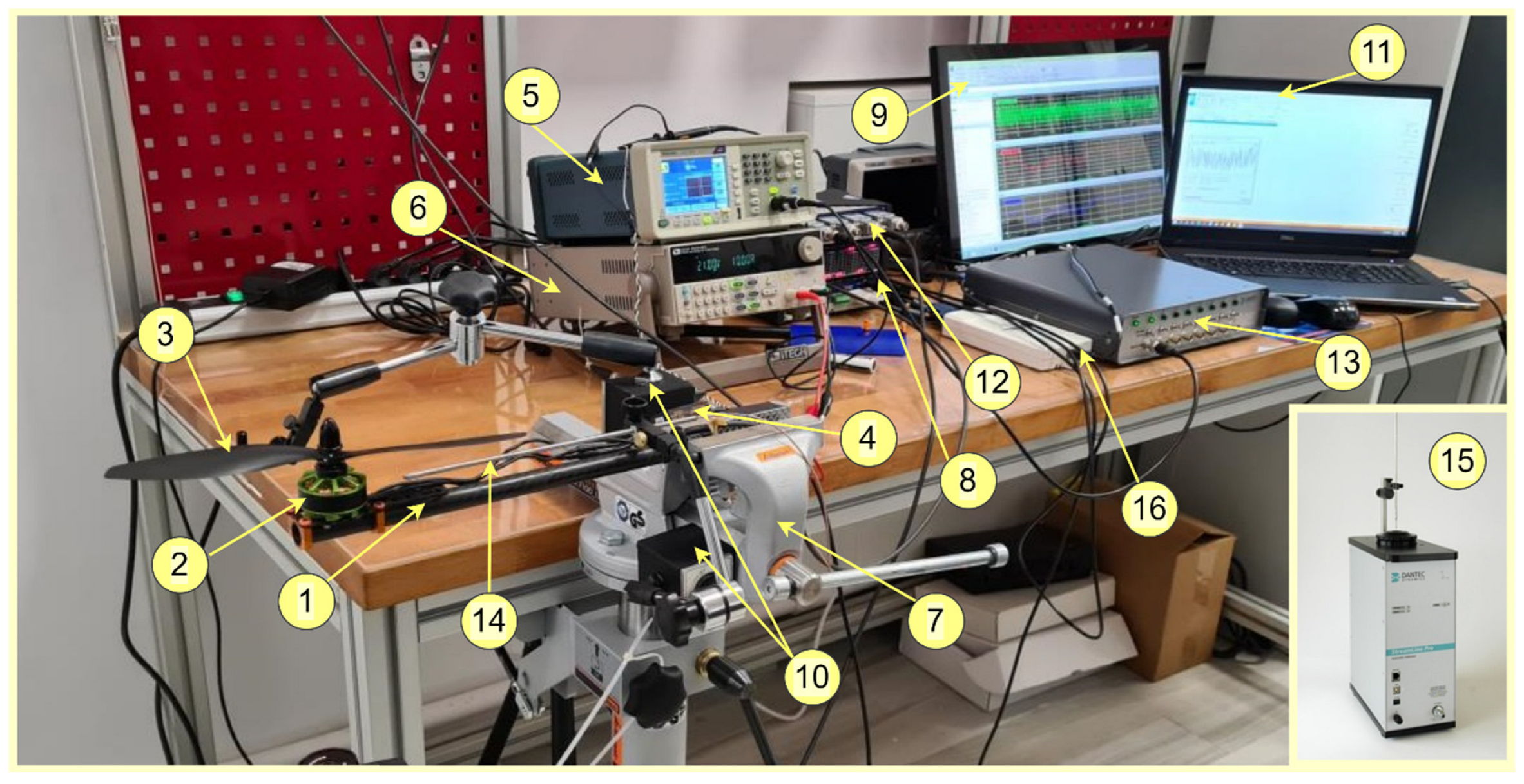
2. Materials and Methods

The experimental tests carried out in the present research consisted of the determination of the velocity fields and the turbulence intensity measured at different points of the working fluid (air) driven into motion by the motor–propeller assembly of a Tarot Iron Man 650 quadcopter [25,26]. The experimental setup for testing the quadcopter arm is shown in Figure 1.
The experimental setup for testing the quadcopter arm is divided into two equipment categories. The categorization thus marks the type of measurement for which the equipment was used.
The first category of equipment is the stand, which aims to drive the electric motor in rotation and includes the following components:
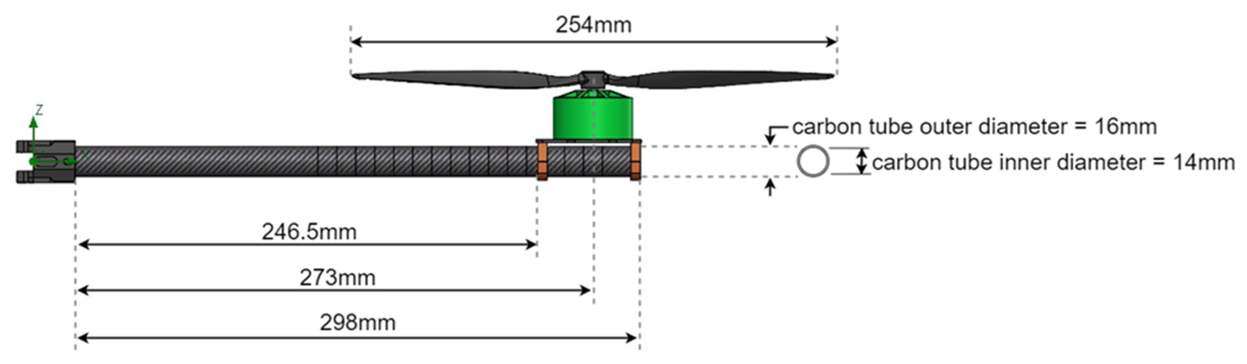
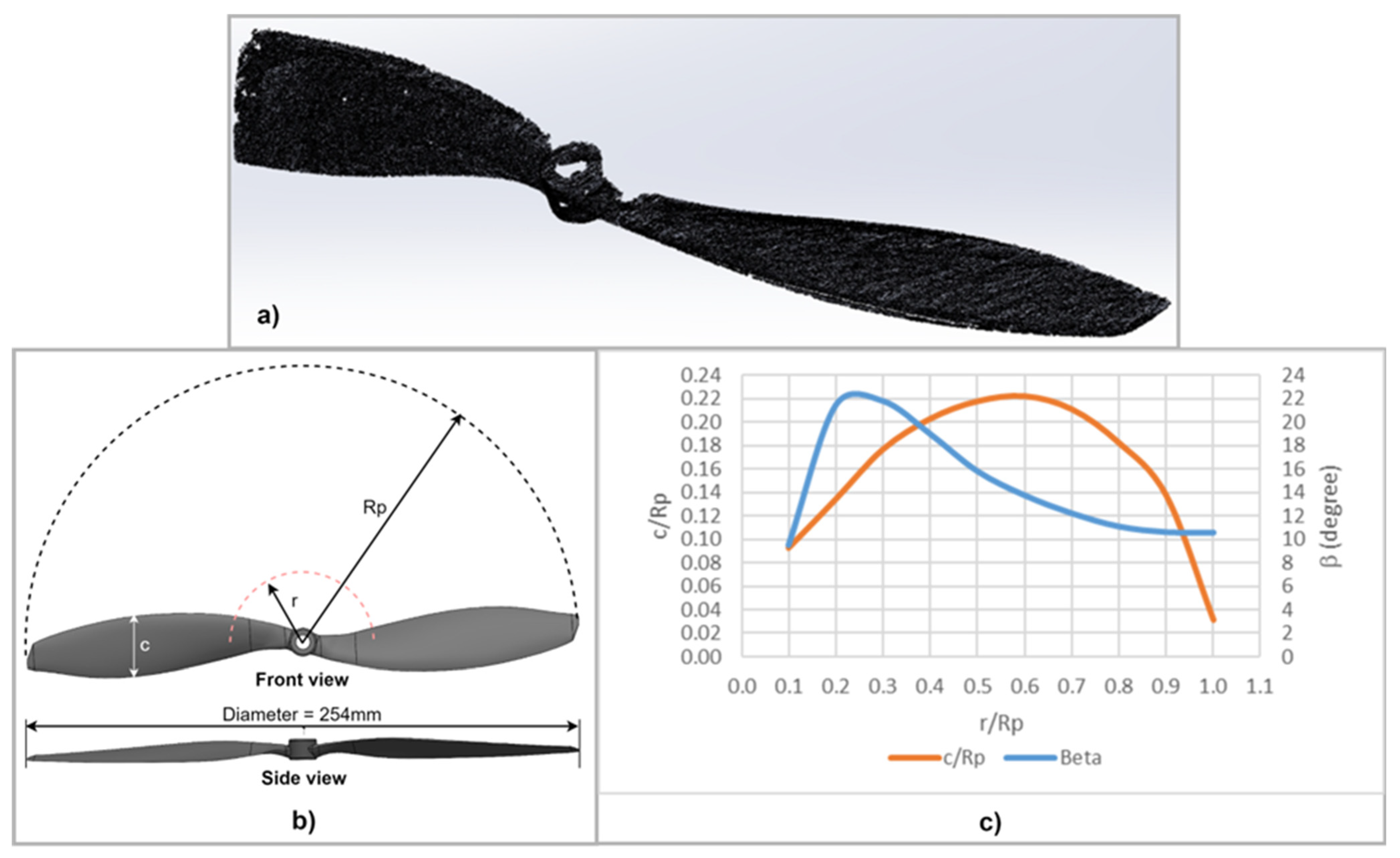
  • motor–propeller assembly: (composed of TURNIGY Multistar 3508 640 v2 brushless electric motor and Multistar propeller with DJI adapter 254 × 114 mm);
  • esc: HOBBYWING XRotorPro50A ESC (ESC = electronic speed controller, which was used to control and regulate the speed of the electric motor);
  • the signal generator: TEKTRONIX-AFG1062 (through which, the step-type signal was introduced to drive the motor with the following characteristics: frequency of 500 Hz, power/duty cycle 50%, start phase 0°, amplitude 5 Vpp, compensation 2.5 V);
  • voltage source: ITECH IT6722A 400 W DC with 80 V 20 A power supply (through which, 21 V voltage and 10 A electric current were introduced to drive the electric motor).
The second category is made up of the equipment used to obtain the velocity and turbulence fields measured at different points of the working fluid (air) driven into motion by the motor–propeller assembly for the different operating modes of the motor, and contains the following components:
  • the signal amplifier: QuantumX MX840B from HBM (used to amplify the measurement data acquired by the anemometer);
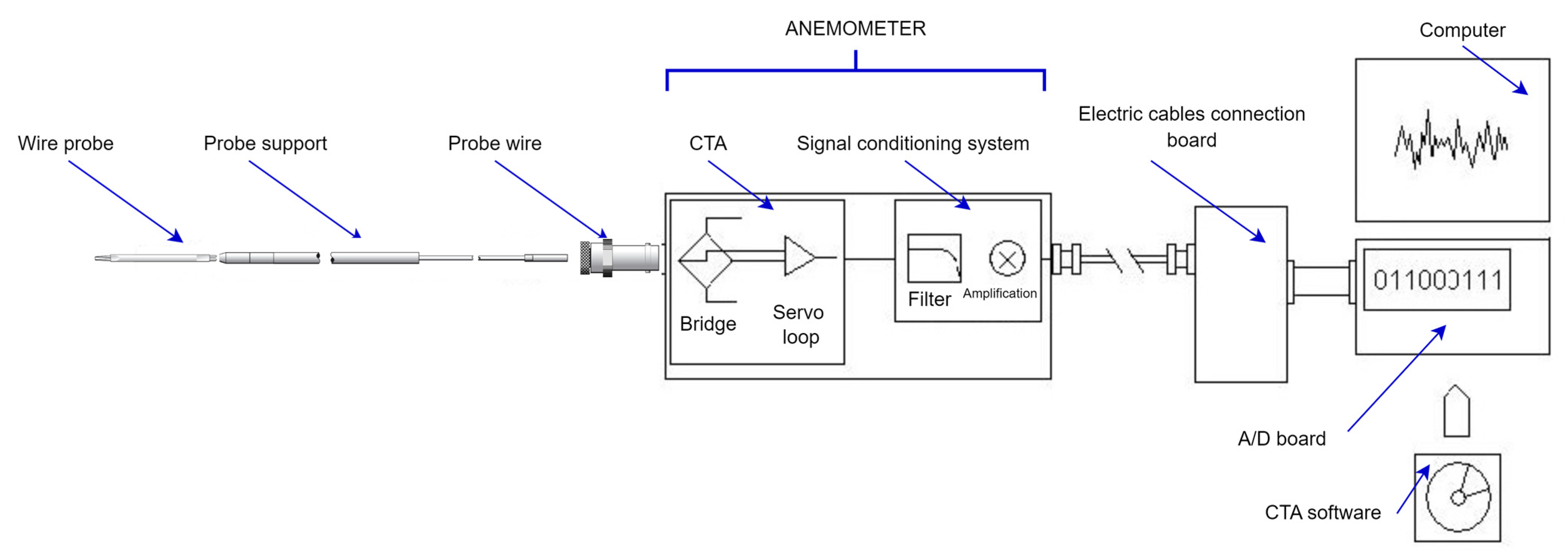
  • hot wire anemometer: MultiChannel CTA 54N80 from Dantec Dynamics (CTA = constant temperature anemometer—multi-channel constant temperature anemometer was used to measure the speeds at different points of the air jet produced by the engine–propeller assembly in the vicinity of the quadcopter arm);
  • miniature wire probes: 55P11 (used together with the anemometer of acquisition board: National Instruments NI USB-6212 (used for real-time viewing in StreamWare Basic software V6.50 of the results recorded by the anemometer);
  • supports for probes with a single sensor: 55H21 (used together with the anemometer for recording the velocity field of the air jet);
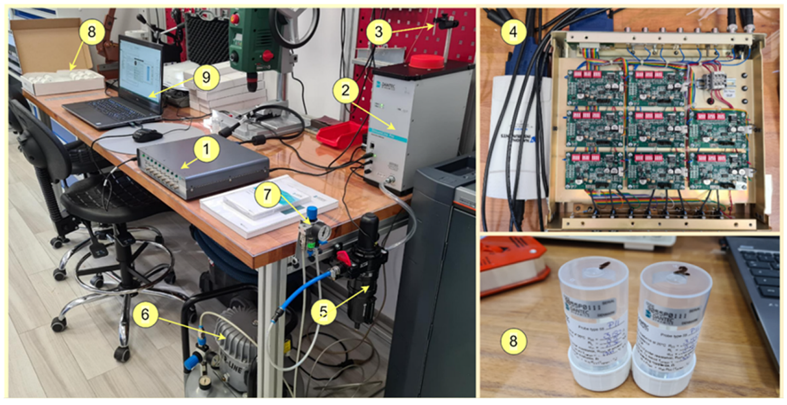
  • the anemometer calibration system: StreamLine (used to calibrate the miniature wire probes before and after each experimental test);
  • acquisition board: National Instruments NI USB-6212 (used for real-time viewing in StreamWare Basic software of the results recorded by the anemometer);
  • the computer: for running the StreamWave Basic software (software used together with the anemometer to measure air speeds in real time);
  • the computer: for running the CATMAN-HBM software 5.5.3 (software used to display and interpret the results of measuring the speeds acquired from the anemometer).
An important step prior to sensor calibration and measurement data acquisition is the hardware configuration of the CTA, which involves adjusting the superheat ratio [27,28]. This superheat ratio determines the operating temperature of the sensor, which the producer recommends to be equal to 0.8 for air fluid, and is defined as:
a = R s , h o t R s , c o l d R s , c o l d
where R s , c o l d is the cold resistance of the sensor at T 0 and is provided by the manufacturer for each individual sensor, where T 0 = 22 ° C is the reference ambient temperature; R s , h o t is the thermal resistance of the sensor at the operating temperature of the sensor T w , and results in R s , h o t .
Thus, the operating temperature of the sensor, T w , which is determined by the superheat ratio, is defined as:
T w = ( R s , h o t R s , c o l d 1 ) ( 1 + α 20 ( T 0 T 20 ) α 20 ) a ( 1 + α 20 ( T 0 T 20 ) α 20 )
where α 20 is the temperature coefficient of the temperature sensor resistance T 20 = 20 ° C and is provided by the manufacturer for each individual sensor.
Another important component in the hardware configuration of the CTA is determining the overheat resistance (the value that is held constant by the servo loop in the CTA) and the decay resistance (the value that settles in the bridge and causes the sensor to overheat) [29,30]. The resistance to overheating is determined as follows:
R o v e r h e a t i n g = R s , h o t + ( R c o n e c t o r s + R s u p p o r t + R c a b l e ) ,
where R c o n e c t o r s is the resistance of the probe connectors and is provided by the manufacturer for each individual sensor; R s u p p o r t is the resistance of the probe holder; R c a b l e is the resistance of the BNC cable.
Decadal resistance is defined as:
R d e c a d e = R P R o v e r h e a t i n g ,
where RP is the bridge ratio for multichannel CTA.

3. Results

3.1. Determination of Air Jet Velocity Variations in the Vicinity of the Quadcopter Arm Generated by Propellers in Rotational Motion in Engine Operating Regimes Resulting from Experimental Testing

The multichannel CTA hot wire anemometer from Dantec Dynamics was used to determine the variation in the air jet velocity in the vicinity of the quadcopter arm generated by the propeller in the rotational motion for the engine operating regimes. The instantaneous flow velocity measurement using the CTA anemometer is based on the heat transfer between the probe sensor (a thin electrically heated tungsten wire) and the fluid medium around the quadcopter arm [31]. The rate of heat loss depends on the temperature surplus of the sensor, its physical properties, geometric configuration, and the properties of the moving fluid [32].
This system for measuring fluid velocities consists of a measuring chain (Figure 2) and contains a sensor probe, a probe support, a probe cable, a CTA anemometer, a signal conditioning system, a converter A/D (ana-log/digital), a data acquisition board, and a computer used to run a dedicated software application for configuring the CTA and analyzing the acquired data called StreamWare Basic [33,34]. In addition, a dedicated automatic probe calibration system named StreamLine was additionally used to ensure proper interpretations of acquired data and to speed up the experiments, thus reducing total costs.
The selection of the probe type provided for compliance with the environmental conditions was: gaseous fluid (air); the number of velocity components that need to be measured (a component); expected velocity range (0.5 m/s–20 m/s); the parameter for measurement (vi-thesis); the required spatial resolution; the intensity of the turbulence (5–10%) and the frequency of fluctuation in the flow (choosing a probe that ensures a frequency as high as possible); temperature variations; risk of contamination; the available space around the measuring point (free flow). Thus, the 55P11 single-wire miniature probes were best suited for these types of measurements, and their connection to the CTA was made through a 55H21 probe holder and a model A1863 BNC cable.

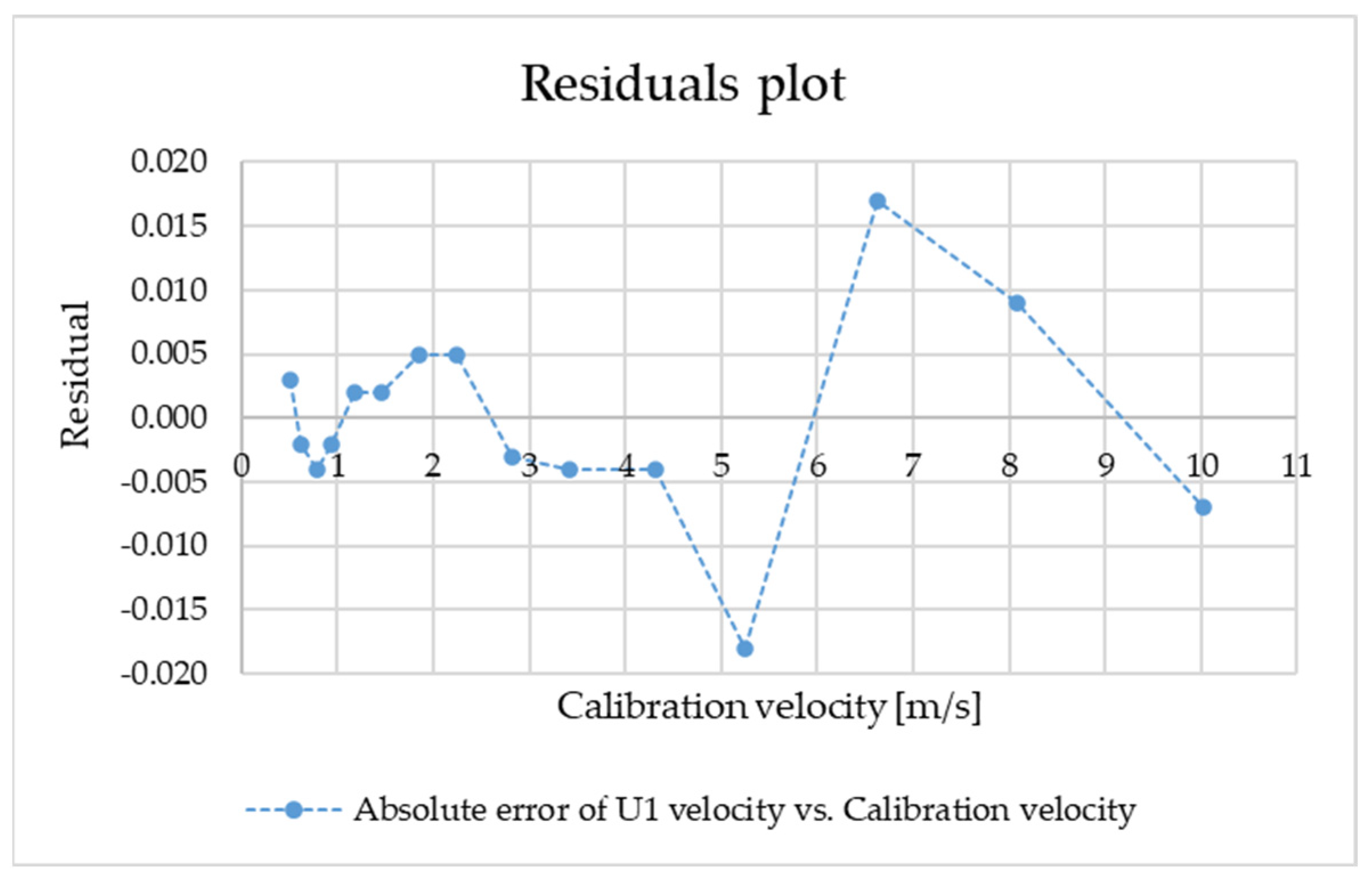
3.1.1. Calibration of Sensors

The relationships were used for the calculations required to calibrate the sensors (1–4):
a = R s , h o t R s , c o l d R s , c o l d = 0.8
where R s , c o l d = 3.5 Ω at T 20 = 22 ° C , which is the reference ambient temperature; T w 300 ° C (value given by the manufacturer; see “8 in Figure 3” —wire probes) results in R s , h o t = 6.3 Ω .
Thus, the operating temperature of the sensor, T w , is:
T w = a ( 1 + α 20 ( T 0 T 20 ) α 20 ) = 242 ° C ,
where α 20 = 0.36 % / ° C (value given by the manufacturer; see “8 in Figure 3” —wire probes) for T 20 = 20 ° C .
Another important component in the hardware configuration of the CTA is determining the overheat resistance (the value that is held constant by the servo loop in the CTA) and the decay resistance (the value that settles in the bridge and causes the sensor to overheat) [33,34]. The resistance to overheating is determined as follows:
R o v e r h e a t i n g = R s , h o t + ( R c o n e c t o r s + R s u p p o r t + R c a b l e ) = 7.44 Ω ,
where R c o n e c t o r s = 0.5 Ω ; R s u p p o r t = 0.44 Ω is the resistance of the probe holder 55H21; R c a b l e = 0.2 Ω is the resistance of the BNC cable for the length of 4 m.
Decadal resistance is defined as:
R d e c a d e = R P R o v e r h e a t i n g = 148.8 Ω ,
where RP is the bridge ratio of 1:20 for multichannel CTA.
For the proper interpretation of the voltage data captured from the sensors of the CTA probes, a calibration of the sensors was carried out using the StreamLine calibration system. The calibration procedure establishes a relationship between the CTA voltage output (in volts) and flow velocity (in m/s). This calibration was performed by exposing the probe to a set of known velocities, U, for which, the corresponding voltages, E, are recorded speeds.
The calibration chain used is shown in Figure 3. The probe was mounted in the calibration device with the probe connectors oriented parallel to the air jet. The ambient conditions, temperature (T) and barometric pressure (P), were automatically recorded by the device. The chosen configuration for the calibrator to operate is a superheat adjustment calibration procedure, which involves balancing the bridge prior to calibration and establishing a new superheat configuration using the same superheat ratio as that originally established. The minimum (Umin,cal) and maximum (Umax,cal) calibration speeds were set according to the range of speeds expected to be captured by the sensors in the experimental measurements, and the number of calibration points were chosen so that the calibration curve contains as many landmarks as possible for plotting. Therefore, 15 calibration points were chosen, and the type of velocity distribution chosen was the fourth-order polynomial distribution.
The data captured from the probe sensor are shown in Table 1, where Ugenerated is the velocity corresponding to the calibration point generated by the polynomial distribution selected in StreamWare Basic, U is the measured velocity, E1 is the sensor voltage recorded in the CTA, T is the received temperature, P is the atmospheric pressure, and U1calc is the calculated velocity.
Figure 4 and Figure 5 show the calibration curve and the diagram of the residuals obtained by a calculation algorithm similar to that of the CTA software - StreamWare Basic software V6.50 but obtained in the Mathcad software 14.0 and graphically plotted.

3.1.2. Recording Measurement Data from CTA

For velocity data acquisition, the CTA anemometer was connected in the data acquisition chain from the HBM via the anemometer’s MonitorOut.
The algebraic form of the polynomial, which constitutes the transfer function, is:
U = f ( E ) = C 0 + C 1 E + C 2 E 2 + C 3 E 3 + C 4 E 4 ,
Following sensor calibration, a function channel was created in the Catman software- StreamWare Basic software V6.50 (of the HBM procurement chain), where the recorded velocity U was defined as a fourth-order polynomial function in the undetermined E (voltage recorded by output) with the following polynomial coefficients:
C 0 = 24.58374 C 1 = 67.8181 C 2 = 61.638233 C 3 = 18.528749 C 4 = 0.000003 ,
The measurements performed for the acquisition of data related to the variation in the air jet velocity in the vicinity of the quadcopter arm were carried out in the fixing positions of the CTA probe shown in Figure 6 and Figure 7.
Measurements I—sensor in the direction perpendicular to the arm and propeller axis at a distance of 75 mm (data acquisition starting from r = 0 mm to r = 140 mm from 20 mm to 20 mm).
Measurements II—sensor parallel to the arm at a distance of 25 mm (data acquisition starting from r = 25 mm to r = 135 mm from 10 mm to 10 mm).

3.1.3. Analysis of Data Acquired with the CTA Anemometer

The signal recorded from the CTA sensor in a turbulent flow is random in nature, which creates the need for a statistical description of the signal. The time series can be analyzed in the amplitude domain, time domain, or frequency domain. All three types of procedures require random stationary data for analysis.

Analysis of Data in the Amplitude Domain

Amplitude domain analysis provides information about the amplitude distribution in the signal and is based on one or more time series sampled on a single integral time scale in the fluid flow (time scale characteristic of fluid velocity measured in turbulent flow). A velocity time series represents data from a sensor converted to a velocity component in engineering units. A single velocity time series provides mean moments, root mean square moments, and higher-order moments.
From the moments based on a single time series, the following are obtained:
  • The average value of the velocity (the first-order moment of the statistical series):
U a v e r a g e = 1 N 1 N U i ;
  • The standard deviation of the velocity (defined as the second-order moment of the statistical series), also called the root mean square deviation of the velocity, which is determined as a simple mean square of the deviations of the values of the series from their mean, with the result representing the square root of the variance:
U r m s = 1 N 1 1 N ( U i U a v e r a g e ) 2 ;
  • The variance, also called the dispersion (defined as the second-order moment of the statistical series), which represents the turbulent kinetic energy per unit mass at a given point and is calculated as a simple arithmetic mean of the squares of the deviations of the terms of the series from their trend plant:
σ 2 = 1 N ( U i U a v e r a g e ) 2 N 1 ;
Table 2 shows only two cases, corresponding to measurement position I at the distance r = 0 mm (on the propeller axis) and, respectively, measurement position II at the distance r = 25 mm from the propeller axis for the operating regimes of the engine of 60%, 70%, 80%, and 90%.
Figure 8 shows the description of the geometry of the quadcopter arm and the dimensions of the propeller used in the present study.
Figure 9 shows the variation in engine traction according to its experimentally determined speed.

3.2. Numerical Analysis

The variation in the velocity of the air jet produced by the propeller in the vicinity of the quadcopter arm constituted by the tube of composite material with carbon fiber twill fabric reinforcement and an epoxy matrix [35] is analyzed in this subchapter. The numerical simulations carried out consisted of determining the time variation of the velocity distribution developed by the propeller in the rotation movement for the different operating cycles (supply) of the engine. The objective of the study is to determine the pressure distribution on the support arm of the motor–propeller assembly. The pressure distribution was obtained using the fluid flow analysis package of SolidWorks software (version number 2020) to obtain solutions to the Navier–Stokes equations governing the motion of the propeller-entrained air.
The fluid flow analysis using FlowWorks under SolidWorks involved the realization of a series of numerical simulations that follow the same steps, namely: setting up the flow simulation project, initializing the discretization (mesh), setting the calculation control options, choosing the objectives, running the calculations, and analyzing the results (results that, when not providing an acceptable solution due to discretization, led to its refinement).
The software uses the finite volume method, and the fluid mechanics equations are written based on Euler’s formulation. To define the complex geometry of the helix, the ATOS optical measurement system used for object digitization was used [36,37].
Figure 10 shows the meshing of the propeller resulting from the 3D scan, which was later used to create the CAD geometry of the SolidWorks model. The 254 mm diameter of the propeller exceeding the active surface of the scanning platform required the complete scanning (both on the external face and on the internal face) of only one blade.

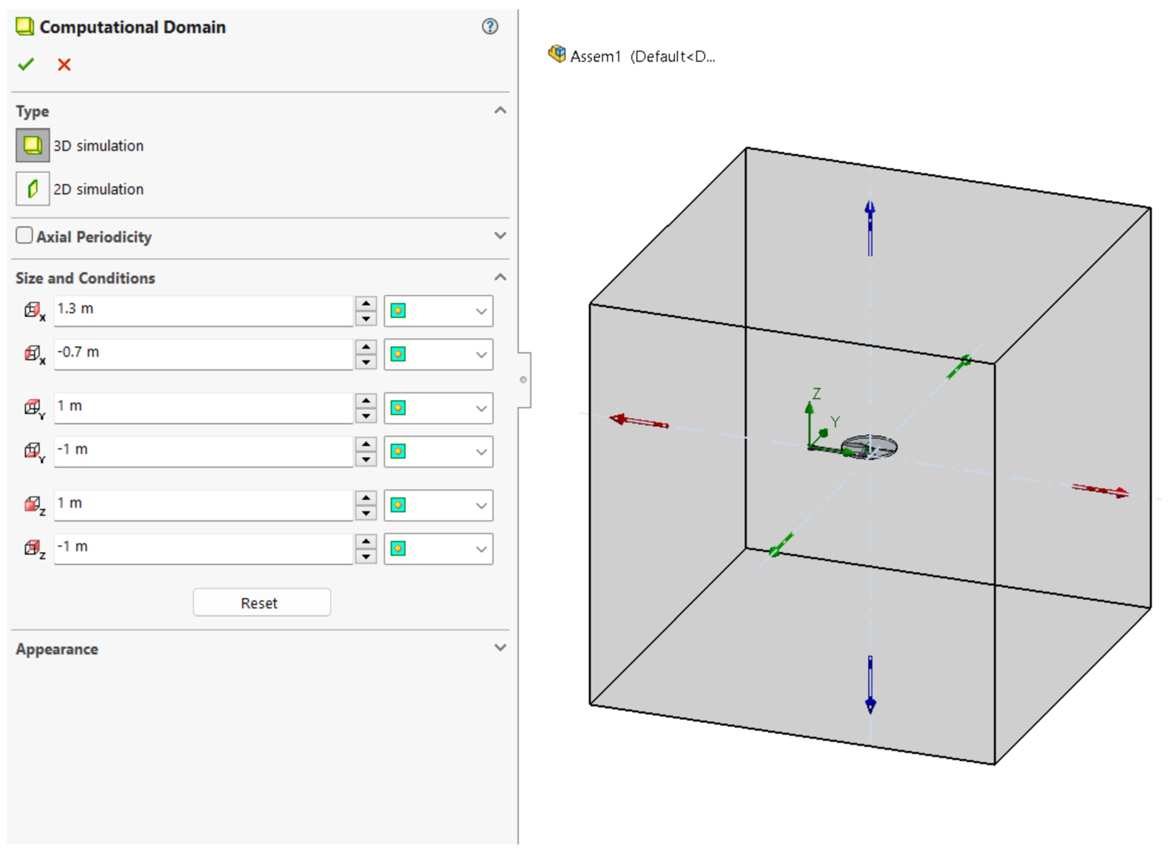
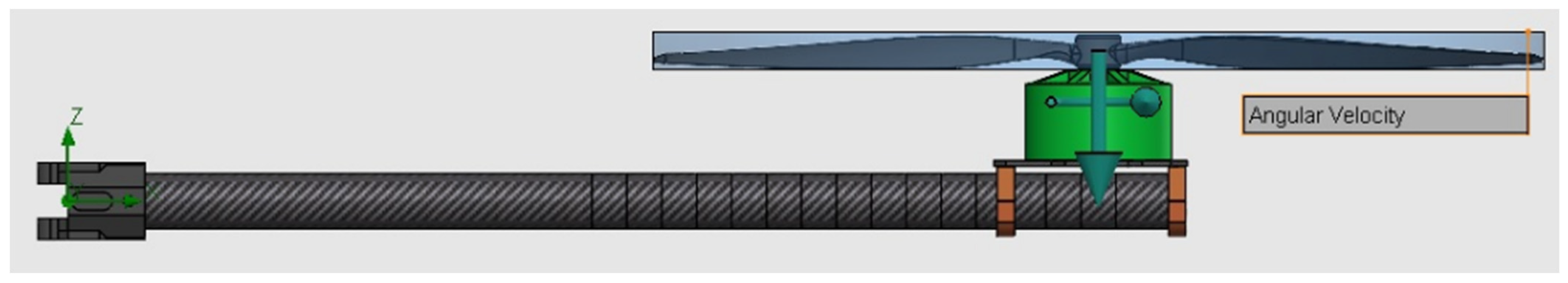
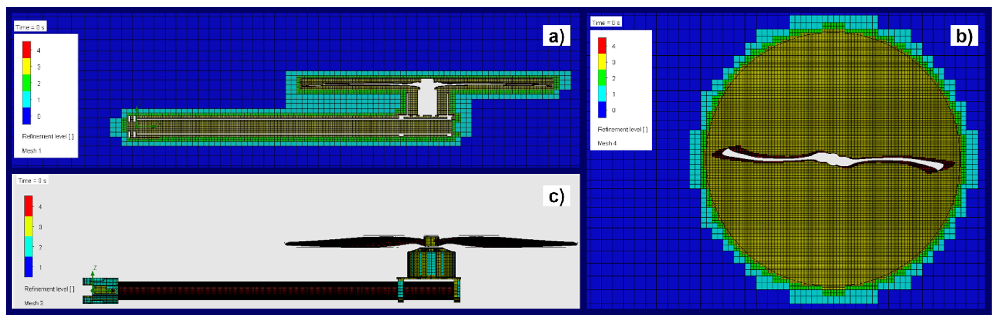
3.2.1. Input Parameters

Carrying out four series of numerical simulations was necessary in order to obtain the different variations in the pressure force distribution corresponding to the four power (operating) cycles of the studied engine. These cycles that were established to be numerically analyzed were validated by experimental measurements made in the laboratory and had the propeller rotation velocity (RPM) as a parameter of variation.
The series of numerical simulations assumed the same configurations for the flow simulation, and external the flow analysis was chosen. The types of flows for the trade wind were both laminar and turbulent. The initial conditions selected were atmospheric pressure 1 bar and temperature 23 °C. The computational domain was defined as a cube with a side of 2 m in the three directions of the x, y, and z axes of the coordinate system as shown in Figure 11.
Setting the physical characteristics included opting for a time-varying and rotating sliding mesh flow. Using the sliding mesh method, the areas of the motor rotor together with the propeller and those of the stator together with the other components of the assembly were connected by a sliding interface. The sliding interface, which coincides with the boundary of the rotating region, must be inside a volume of fluid (volume of rotation defined as in Figure 12).
The discretization in the SolidWorks flow simulation consists of cells in the form of rectangular parallelepipeds and contains fluid cells, partial cells (solid/fluid boundary cells), and solid cells. As the variation in the density of the computational network (mesh) and the study of the convergence of the solution as the network is refined are essential components of any computational study of flows, several variants of discretization were tested, and the solution presented in Figure 13 represents the final variant chosen for numerical analysis.
Thus, the global discretization was performed with a level 7 refinement and two other local discretization’s were added, one for level 4 partial cell refinement for the carbon tube surfaces (representing the quadcopter arm), the propeller surfaces, and the top surface of motor mount plate, and the other for level 3 refinement of the fluid cells belonging to the volume of rotation, resulting in a total of 1,242,056 cells (which are only fluid cells), of which, a number of 111,168 fluid cells are in contact with the solid.
In the calculation control options, it was chosen for all of the objectives to reach convergence, and for the physical analysis time to be the equivalent of at least five complete rotations of the propeller, thus obtaining:
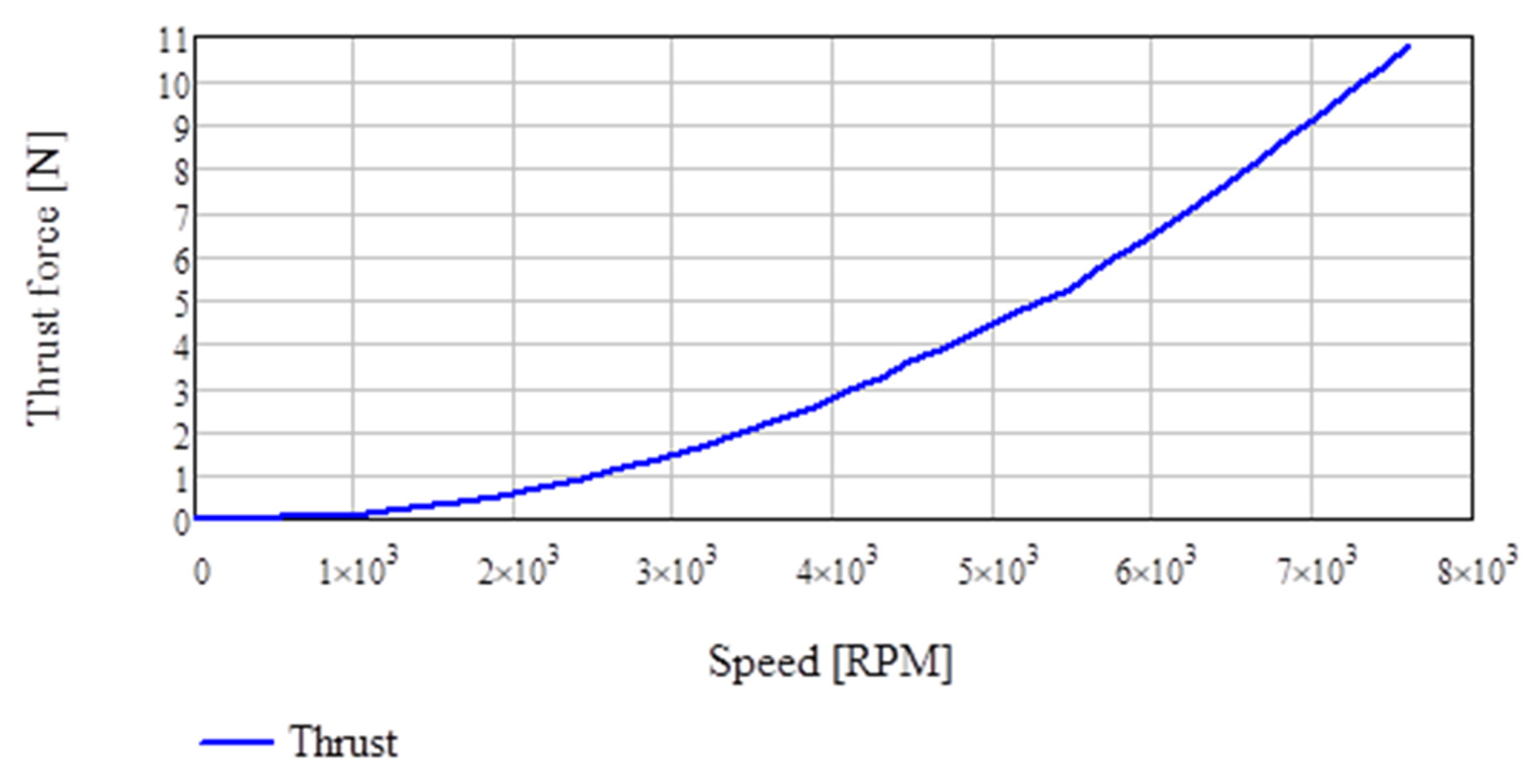
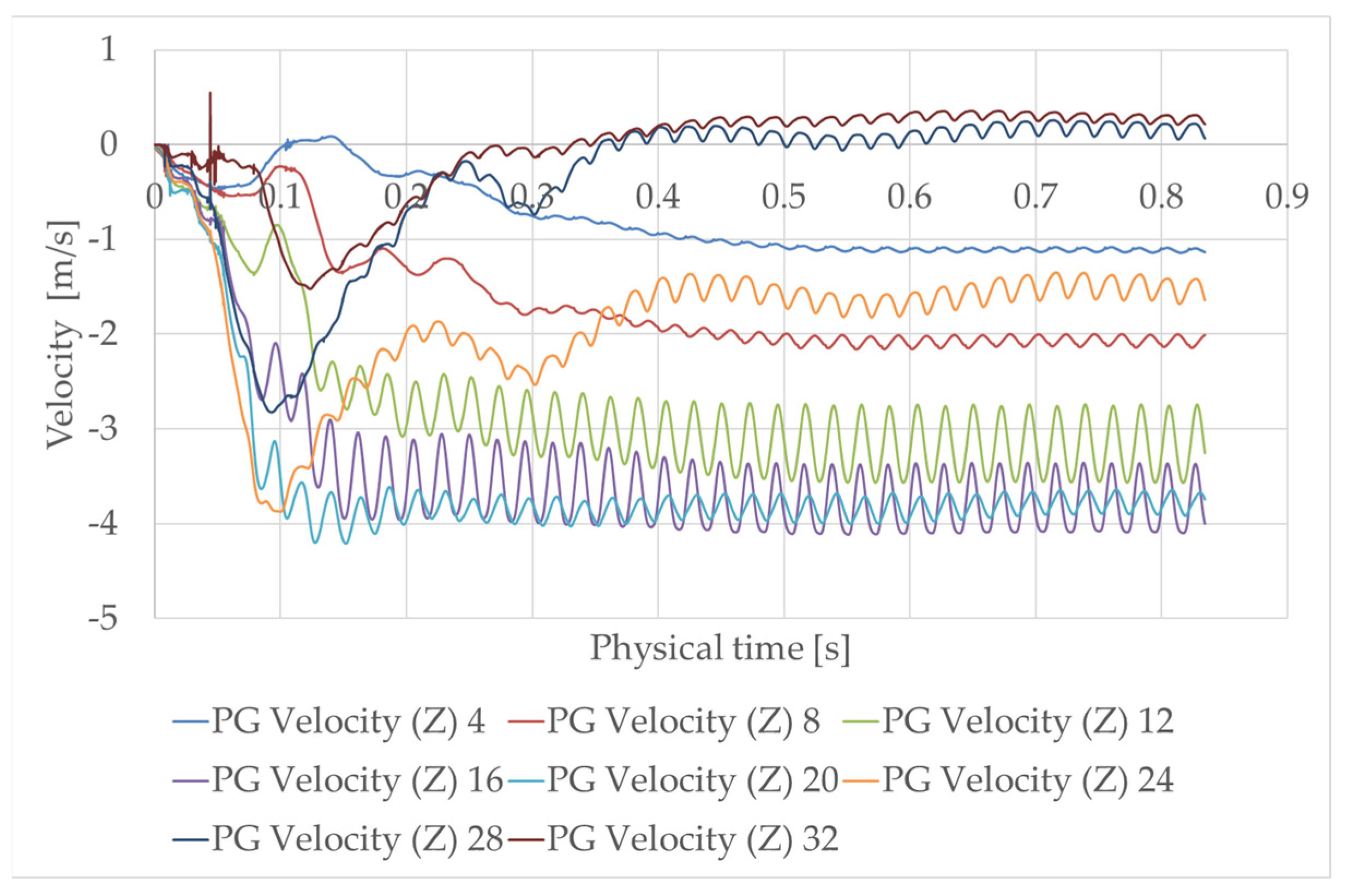
  • For the 60% duty cycle (1350 RPM)—a physical time of 0.834 s was achieved until a periodic transient cycle was identified, and the time step for saving the results was 0.00055 s;
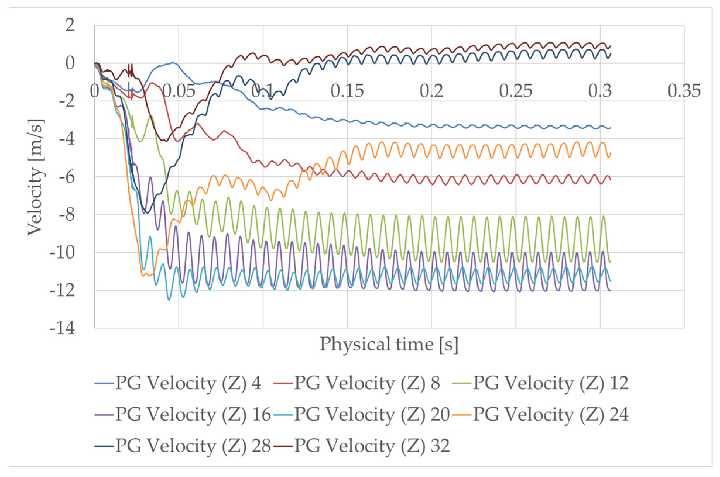
  • For the 70% duty cycle (3900 RPM)—a physical time of 0.306 s was achieved until a periodic transient cycle was identified, and the time step for saving the results was 0.0002 s;
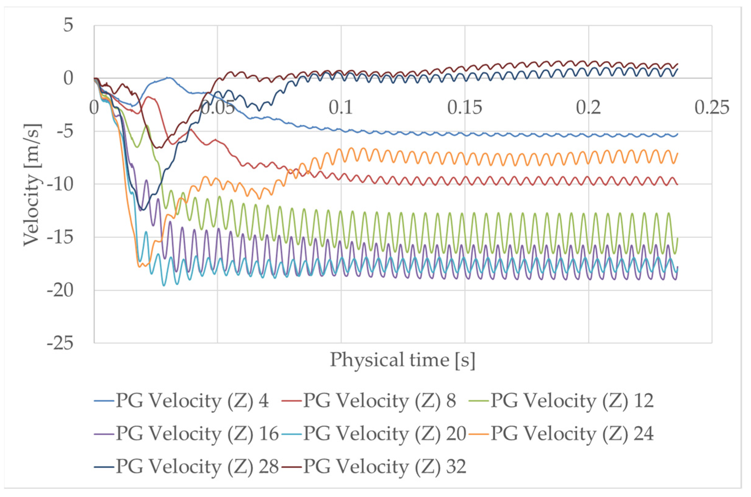
  • For the 80% duty cycle (6100 RPM)—a physical time of 0.236 s was reached until a periodic transient cycle was identified, and the time step for saving the results was 0.000125 s;
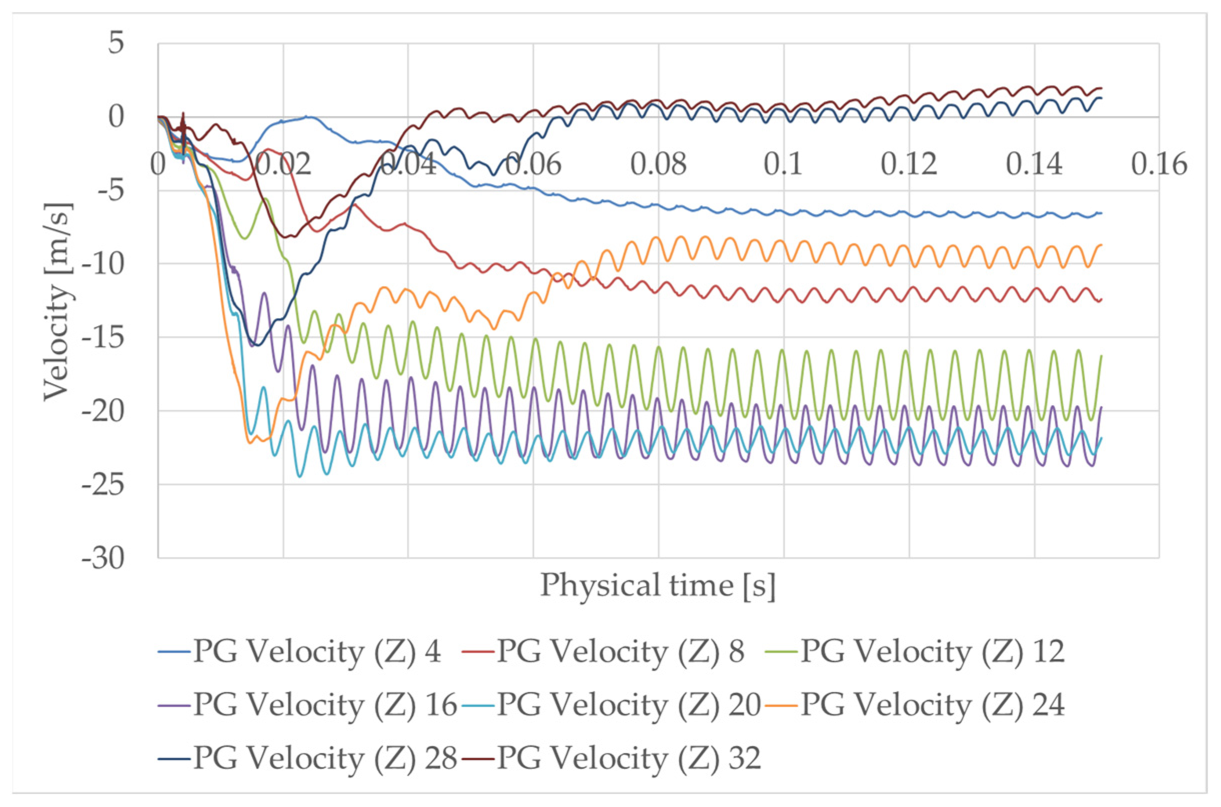
  • For the 90% duty cycle (7600 RPM)—a physical time of 0.151 s was achieved until a periodic transient cycle was identified, and the time step for saving the results was 0.0001 s.
To complete the iterative solution process, a series of objectives were chosen with the aim of minimizing the errors of the calculated parameters and shortening the total solution time. The objectives chosen were both global in nature (pressures, velocities), as well as area objectives and point objectives. The points for which the objectives were set coincide with the points where the experimental measurements were made using the hot wire anemometer (CTA).
The equivalence between the experimental measurement points regarding the velocity components and the velocity component recording points from the numerical flow simulations is presented in Table 3.

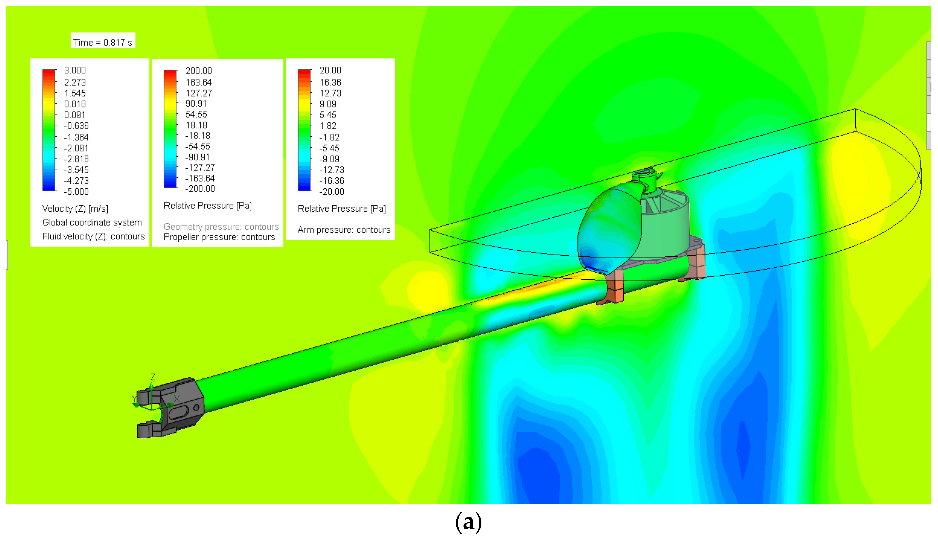
3.2.2. Determination of the Air Jet Velocity Variations Resulting from the Numerical Analysis

Similar to the experimental tests, in the numerical analysis, the variations in the air jet velocity in the vicinity of the quadcopter arm generated by the propellers in the rotational motion in the operating modes of the engine were analyzed. The results of the numerical analysis in the amplitude domain obtained from the CFD study are presented in the following.
The velocity variations at the numerical analysis points equivalent to experimental measurements I and II in the engine power cycle of 60% (1350 RPM), 70% (3900 RPM), 80% (6100 RPM), and 90% (7600 RPM), respectively, are shown in Figure 14, Figure 15, Figure 16, Figure 17, Figure 18, Figure 19, Figure 20 and Figure 21. In Figure 17, Figure 18, Figure 19 and Figure 20, in order to avoid overlapping graphs, only the speed variations in four points were represented.

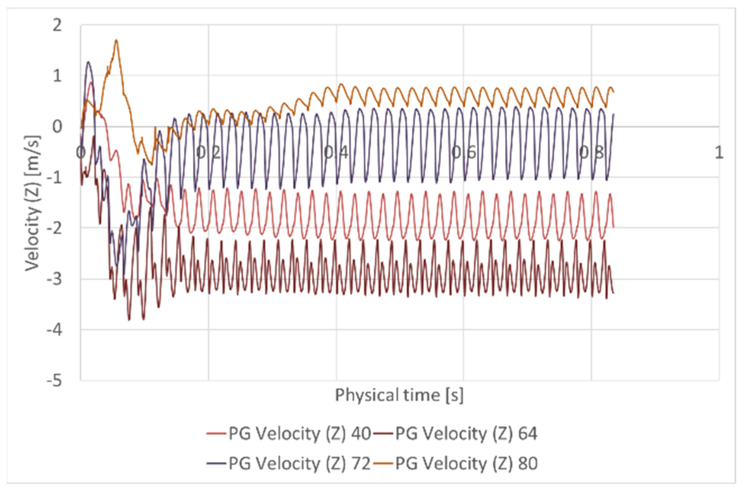
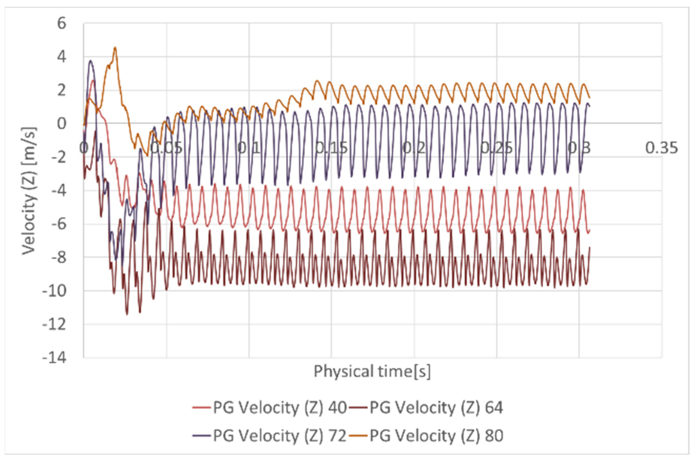
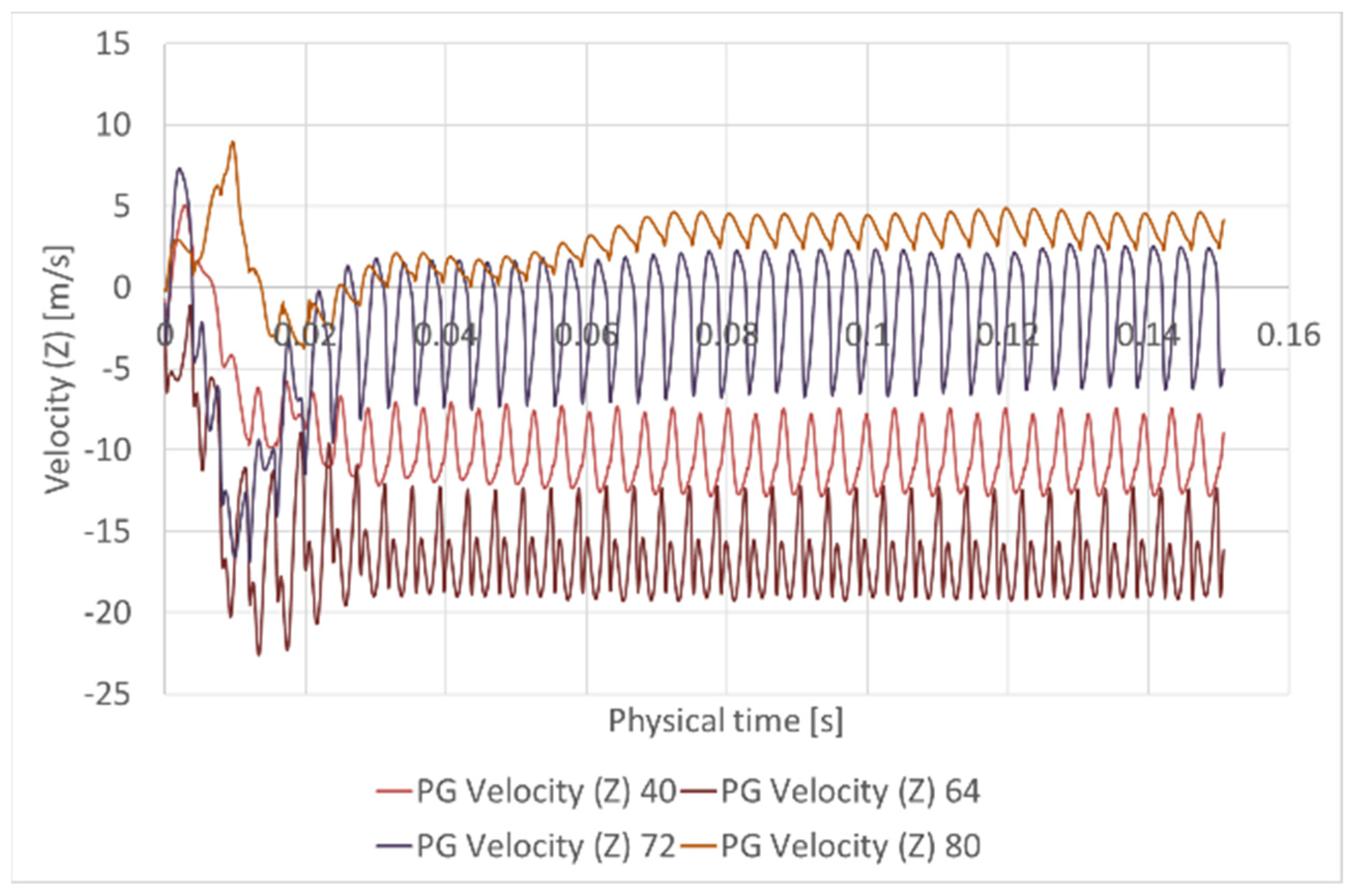
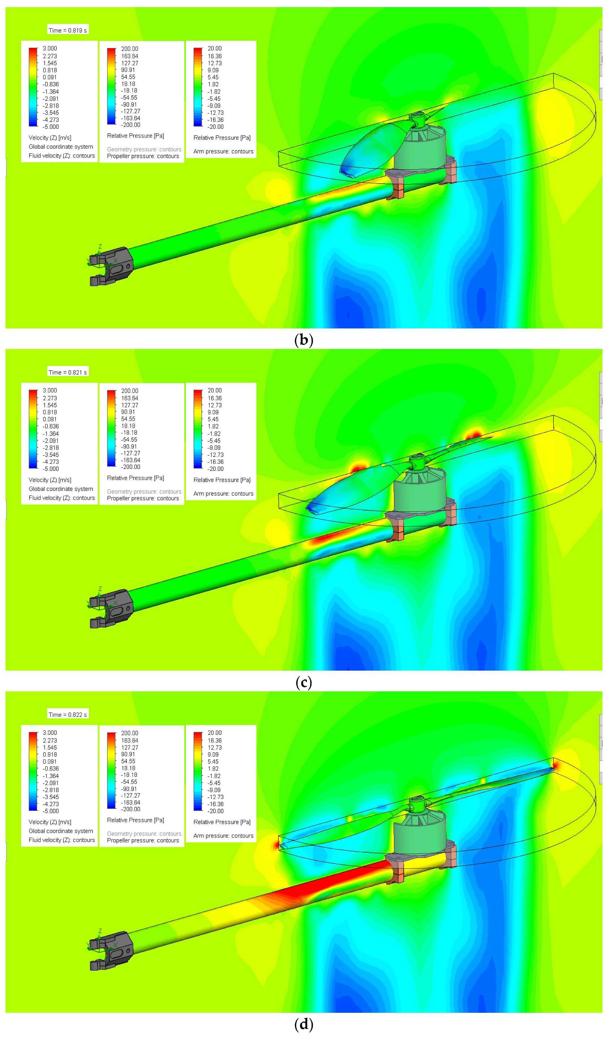
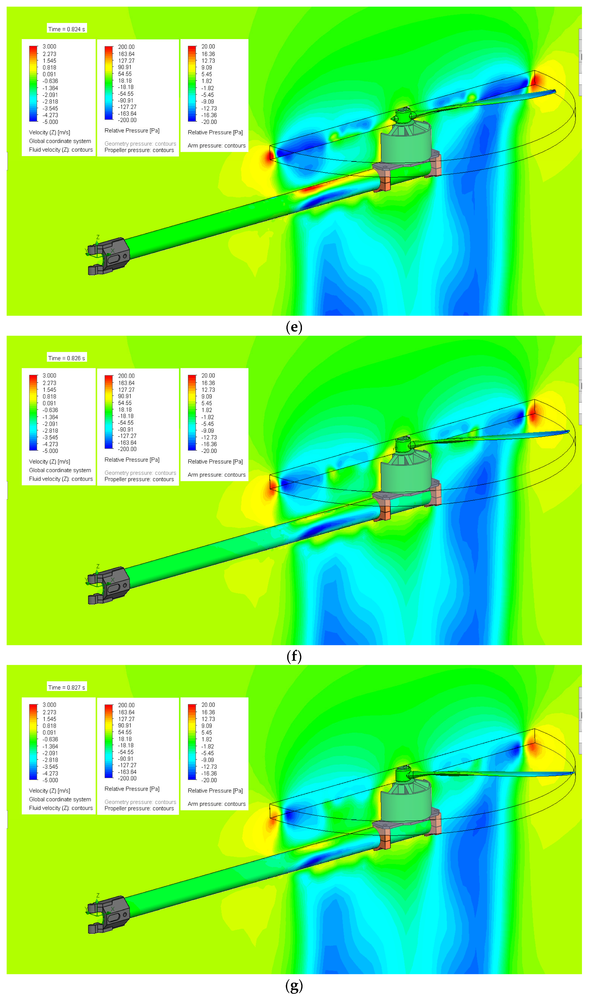
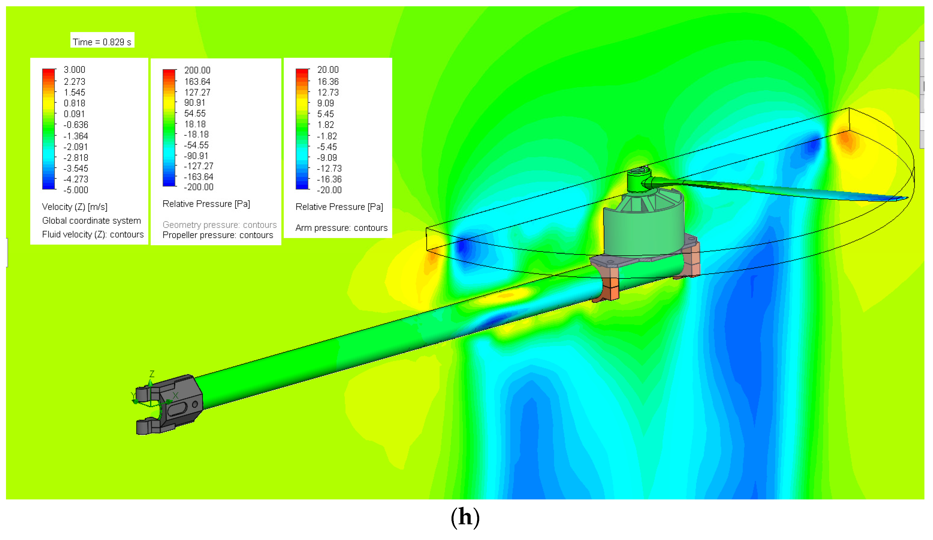
3.2.3. Representation of the Variations in the Air Speed Component in the Z-Axis Direction

In this sub-chapter, the results obtained regarding the variations in the air velocity component in the direction of the Z-axis, the relative pressure on the surface of the quadcopter arm, and the relative pressure on the surface of the propeller for the case of the engine power cycle of 60% (1350 RPM) are presented following a stroke of the propeller blade of 90° from the −45° to +45° angle in relation to the arm (Figure 22).

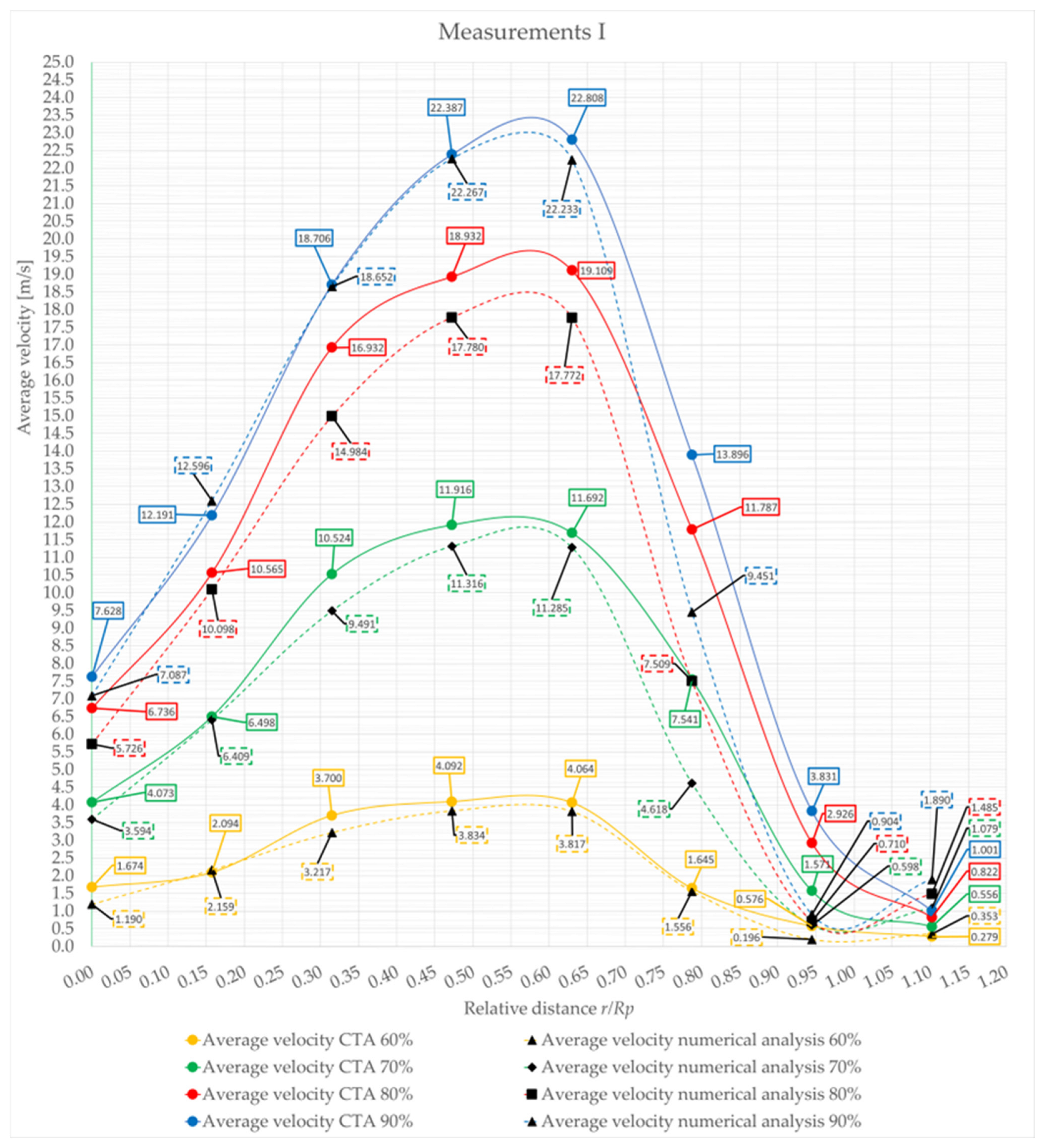
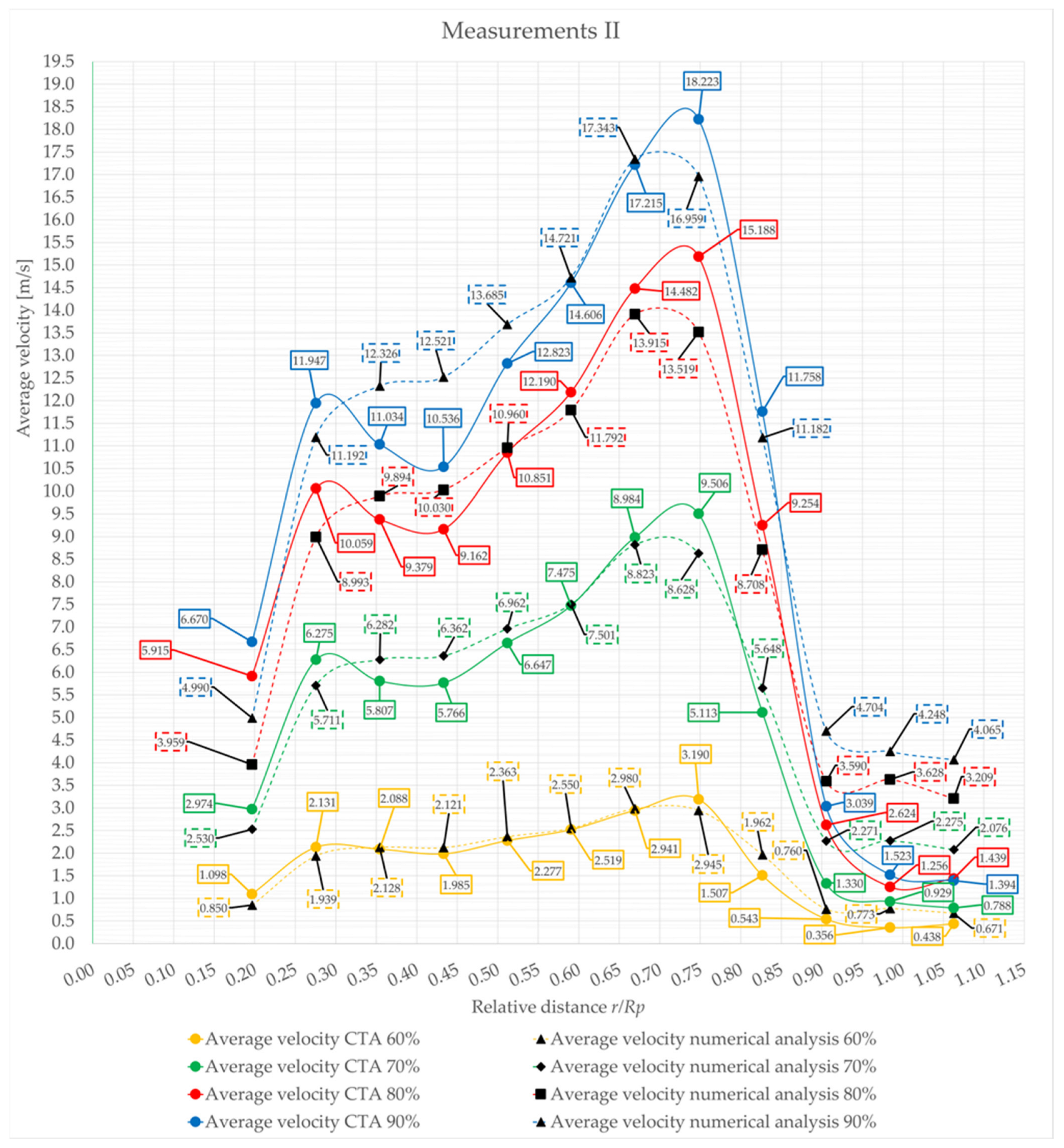
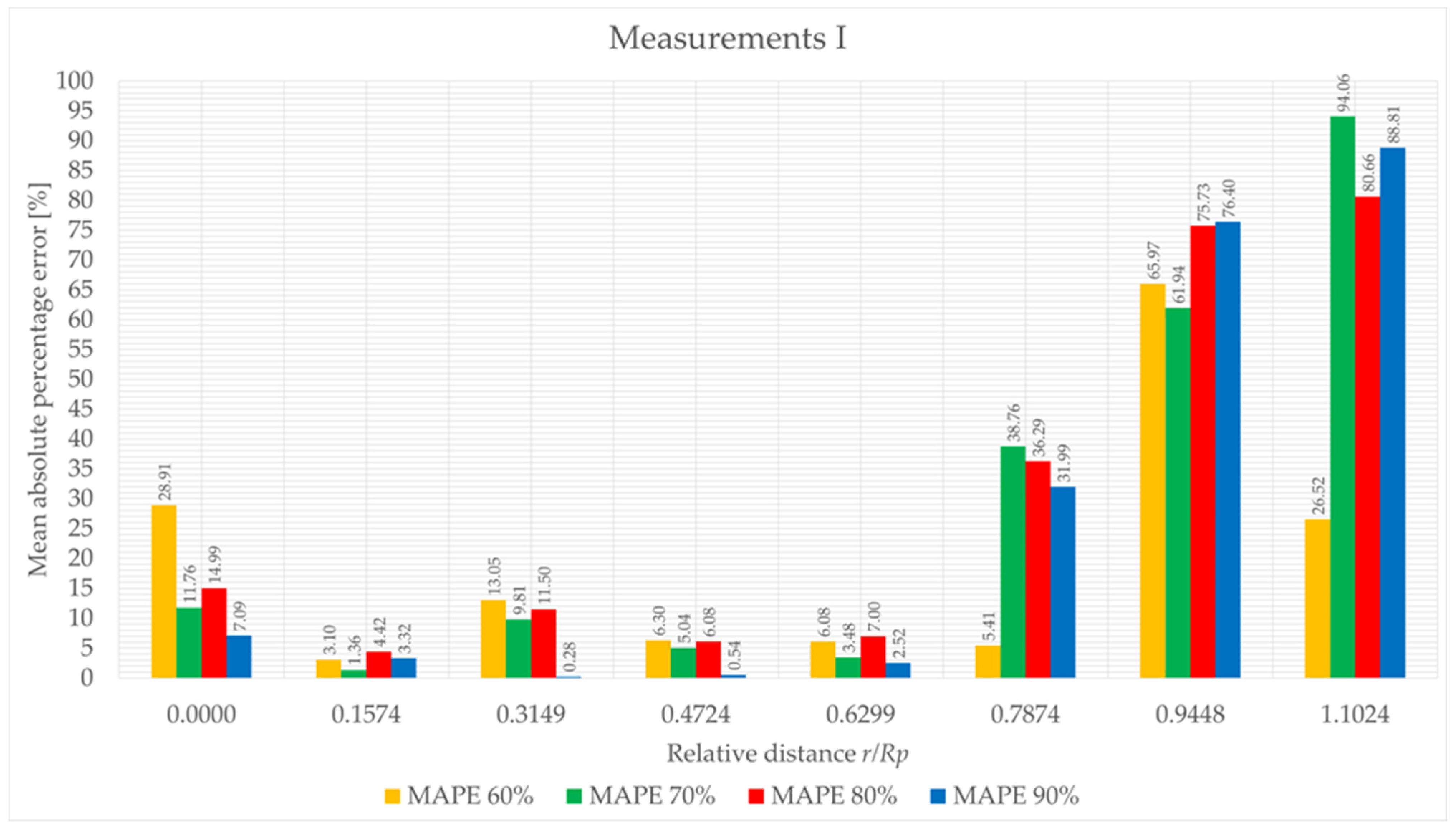
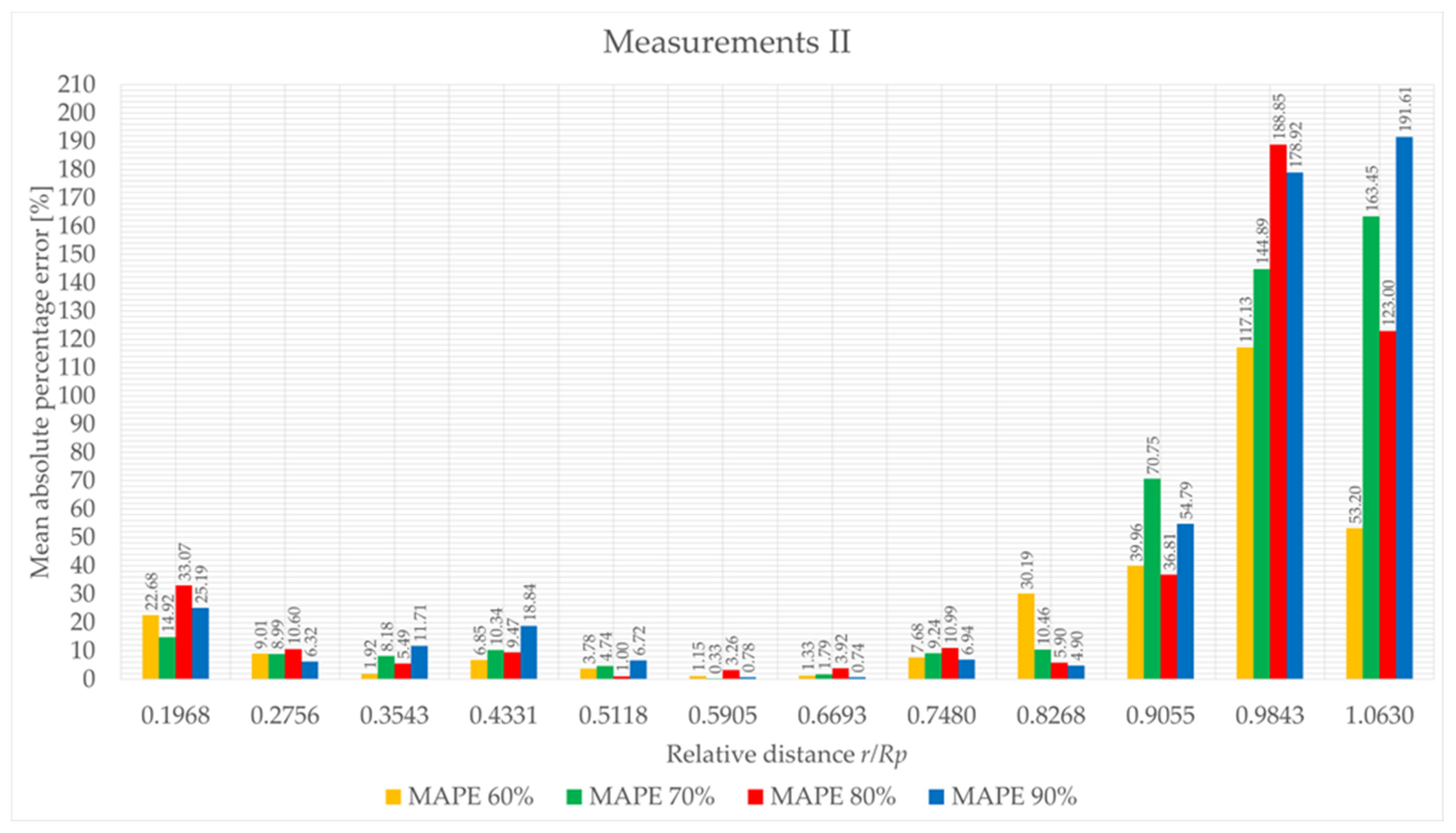
3.3. Comparative Analysis between Experimental and Numerical Results

Following numerical simulations and experimental measurements, the results of the comparative analysis between the average values of the speed measured with the CTA and those obtained from the CFD analysis of the obtained data are presented in Table 4. For the average speed from the CFD analysis, the velocities were composed to obtain a velocity in a plane normal to the direction of the anemometer wire. Thus, for calculation position I, the components of the speed vy and vz were composed, and, in the case of II, the components vx and vz were composed.
The results of the set of measurements I and II of the average speeds determined experimentally with CTA and those determined numerically for the 4 engine operating regimes (60%, 70%, 80%, 90%). Are presented in Figure 23 and Figure 24.
The average absolute percentage error calculated between the results of the set of measurements I of the average speeds determined experimentally with CTA and those determined numerically for the 4 engine operating regimes (60%, 70%, 80%, 90%). Are presented in Figure 25 and Figure 26.

4. Conclusions

From the analysis of the results, it is noted that the agreement between the experimental and simulation results for the set of measurements I is in the range of a 20–80 mm distance from the axis of the propeller, and that the error in this range is around 5%. For a single case in the 20–80 mm interval, at measurement point 12, at a distance of 40 mm from the propeller axis for the engine operating regime of 60%, the error reaches 13%. For r = 0, when the anemometric probe is positioned under the engine, the errors are higher, where the maximum value is 28.91%, corresponding to the engine operating regime of 60%. This can be explained by the fact that the geometry of the motor is not exactly modeled: there are windings (coils) that have not been modeled due to the geometric complexity. For distances from the motor axis greater than 80 mm, the errors increase to approximately 35% for 100 mm from the motor axis at 70%, 80%, and 90% regimes, to approximately 70% at 120 mm, and to 80% at 140 mm.
For measurement set II, a similar behavior is noted. The errors are between 10% and 25% for distances between 25 and 65 mm from the motor axis, fall below 5% for distances between 65 and 85 mm, and start to increase with the distance from the axis, reaching 191% at 135 mm from the front of the motor axis for the 90% motor duty cycle.
This increase in error comes from the insufficient calculation time chosen (the flow has not stabilized) and the insufficient density of calculation cells in the area of interest from the geometric deviations of the components in the model compared to the real ones.
The novelty and scientific contribution of the work lies in the fact that we developed an analytical–numerical model capable of determining the pressure distribution on the drone’s arm for different engine operating modes. The validation of the numerical model was carried out based on a comparison of the speeds determined experimentally with those determined numerically. This allowed us to make structural changes (aerodynamic engine arm) so as to reduce vibrations. The drone is small enough to be used autonomously in order to be able to identify different targets through image interpretation. For this type of mission, the size, quietness in operation, and energy autonomy are essential.
The variable interaction of the air current produced by the propeller with the motor arm represents an excitation factor. Since the experimental determination of the pressures on the upper face of the arm is difficult, an experimental determination of the velocities is necessary for confirming the validity of the numerical calculation. The final goal of the current research, namely the choice of a motor arm with an aerodynamic profile, has been achieved. From our research, it emerged that such an arm profile leads to a reduction in the intensity of the forces and, consequently, to a reduction in the amplitude of the vibrations.

5. Further Directions of Development

In future research, a spectral analysis will also be presented, which is used to provide information on how the signal energy is distributed in the frequency domain. The aperiodic, finite energy signals will be analyzed in the frequency domain using Fourier transform. Afterwards, we plan to design and build an adapter for the quadcopter arm so that the amplitude of the forced vibrations induced by the air jet developed by the motor–propeller assembly is reduced. In addition, we will add other sensors to measure or film the temperature so that we have better control over the thermodynamic state of the propeller propulsion system.
The use of sensors measuring the speed of the hot wire anemometer was not very suitable due to the difficult positioning of the probes in the vicinity of the experimental assembly. In the future, we propose the use of a particle image velocimetry (PIV) device. It would allow for the production of two-dimensional or even three-dimensional vector fields, whereas the anemometer measures the speed only at one point.
Another direction of development is the creation of a dynamic damping system, which uses a piezoelectric actuator to reduce vibrations. The heterogeneous character will be a measurement and control system of a multitude of integrated subsystems depending on the missions that the drone is to perform.
In the future, based on the obtained results, we want to design an aerodynamic motor arm that allows small drones to be used autonomously for various surveillance and monitoring missions. Equipment used for image identification is very sensitive to vibrations. In addition, reducing the noise level will allow the drone to go unnoticed. Another aspect to be pursued is an increase in the reliability of drones.

Author Contributions

Conceptualization, A.T.-N., A.Ș. and L.Ș.G.; methodology, I.O.; software, A.T.-N. and A.Ș.; validation, A.T.-N., A.Ș. and L.Ș.G.; formal analysis, A.T.-N. and A.Ș.; investigation, A.Ș., A.T.-N. and L.Ș.G.; writing—original draft preparation, I.O. and A.T.-N.; writing—review and editing, I.O. All authors have read and agreed to the published version of the manuscript.

Funding

This research received no external funding.

Institutional Review Board Statement

Not applicable.

Informed Consent Statement

Not applicable.

Data Availability Statement

Not applicable.

Acknowledgments

This paper benefited from material support and scientific consulting through the CESATAS—Center of Excellence in Self-Propelled Systems and Technologies for Defense and Security.

Conflicts of Interest

The authors declare no conflict of interest.

References

  1. Krijnen, D.; Dekker, C. AR Drone 2.0 with Subsumption Architecture. In Artificial Intelligence Research Seminar; Leiden University: Leiden, The Netherland, 2014; Available online: https://coendekker.nl/media/pdf/rsai_subsumption_drone.pdf (accessed on 23 November 2022).
  2. Cavoukian, A. Privacy and Drones: Unmanned Aerial Vehicles; Information and Privacy Commissioner of Ontario: Toronto, ON, Canada, 2012; Available online: https://www.ipc.on.ca/wp-content/uploads/resources/pbd-drones.pdf (accessed on 23 November 2022).
  3. Bachmann, R.J.; Boria, F.J.; Vaidyanathan, R.; Ifju, P.G.; Quinn, R.D. A Biologically Inspired Micro-Vehicle Capable of Aerial and Terrestrial Locomotion. Mech. Mach. Theory 2009, 44, 513–526. [Google Scholar] [CrossRef] [Green Version]
  4. Hassanalian, M.; Khaki, H.; Khosravi, M. A new method for design of fixed wing micro air vehicle. Proc. Inst. Mech. Eng. Part G J. Aerosp. Eng. 2014, 229, 837–850. [Google Scholar] [CrossRef]
  5. Hassanalian, M.; Abdelkefi, A.; Wei, M.; Ziaei-Rad, S. A novel methodology for wing sizing of bio-inspired flapping wing micro air vehicles: Theory and prototype. Acta Mech. 2017, 228, 1097–1113. [Google Scholar] [CrossRef]
  6. IMAV 2021 Competition Rules for Indoor and Outdoor Competitions, and Special Challenges. International Micro Vehicle Conference and Competition, [Interactiv]. Available online: https://imav2021.inaoep.mx (accessed on 15 July 2022).
  7. Mohamed, A.; Abdulrahim, M.; Watkins, S.; Clothier, R. Development and flight testing of a turbulence mitigation system for micro air vehicles. J. Field Robot. 2015, 33, 639–660. [Google Scholar] [CrossRef]
  8. Deng, X.; Schenato, L.; Sastry, S.S. Attitude control for a micromechanical flying insect including thorax and sensor models. In Proceedings of the International Conference on Robotics & Automation, Taipei, Taiwan, 14–19 September 2003. [Google Scholar]
  9. Nvss, S.; Esakki, B.; Yang, L.-J.; Udayagiri, C.; Vepa, K.S. Design and Development of Unibody Quadcopter Structure Using Optimization and Additive Manufacturing Techniques. Designs 2022, 6, 8. [Google Scholar] [CrossRef]
  10. Geronel, R.S.; Botez, R.M.; Bueno, D.D. Design and Experimental Study on Vibration Reduction of an UAV Lidar Using Rubber Material. Actuators 2022, 11, 345. [Google Scholar] [CrossRef]
  11. Ge, C.; Dunno, K.; Singh, M.A.; Yuan, L.; Lu, L.-X. Development of a Drone’s Vibration, Shock, and Atmospheric Profiles. Appl. Sci. 2021, 11, 5176. [Google Scholar] [CrossRef]
  12. Zhou, H.; Ma, A.; Niu, Y.; Ma, Z. Small-Object Detection for UAV-Based Images Using a Distance Metric Method. Drones 2021, 6, 308. [Google Scholar] [CrossRef]
  13. Beltran-Carbajal, F.; Yañez-Badillo, H.; Tapia-Olvera, R.; Favela-Contreras, A.; Valderrabano-Gonzalez, A.; Lopez-Garcia, I. On Active Vibration Absorption in Motion Control of a Quadrotor UAV. Mathematics 2022, 10, 235. [Google Scholar] [CrossRef]
  14. Kang, N.; Sun, M. Simulated flowfields in near-ground operation of single- and twin-rotor configurations. J. Aircr. 2000, 37, 214–220. [Google Scholar] [CrossRef]
  15. Raza, S.A.; Sutherland, M.; Etele, J.; Fusina, G. Experimental validation of quadrotor simulation tool for flight within building wakes. Aero. Sci. Technol. 2017, 67, 169–180. [Google Scholar] [CrossRef]
  16. Kaya, K.; Ozcan, O. A numerical investigation on aerodynamic characteristics of an air-cushion vehicle. J. Wind Eng. Ind. Aerod. 2013, 120, 70–80. [Google Scholar] [CrossRef]
  17. Kutty, H.A.; Rajendran, P. 3D CFD simulation and experimental validation of small APC slow flyer propeller blade. Aerospace 2017, 4, 10. [Google Scholar] [CrossRef] [Green Version]
  18. Stajuda, M.; Karczewski, M.; Obidowski, D.; J’ozwik, K. Development of a CFD model for propeller simulation. Mech. Mech. Eng. 2016, 20, 579–593. [Google Scholar]
  19. Zhang, T.; Wang, Z.; Huang, W.; Ingham, D.; Ma, L.; Pourkashanian, M. A numerical study on choosing the best configuration of the blade for vertical axis wind turbines. J. Wind Eng. Ind. Aerod. 2020, 201, 104162. [Google Scholar] [CrossRef]
  20. Joo, S.; Choi, H.; Lee, J. Aerodynamic characteristics of two-bladed H-Darrieus at various solidities and rotating speeds. Energy 2015, 90, 439–451. [Google Scholar] [CrossRef]
  21. ANSYS. ANSYS Fluent Theory Guide; ANSYS: Canonsburg, PA, USA, 2016. [Google Scholar]
  22. Fernandes, N.D.S. Design and Construction of a Multi-Rotor with Various Degrees of Freedom. Master’s Thesis, Technical University of Lisbon, Lisbon, Portugal, 2011. [Google Scholar]
  23. Theys, B.; Dimitriadis, G.; Hendrick, P.; De Schutter, J. Influence of propeller configuration on propulsion system efficiency of multi-rotor Unmanned Aerial Vehicles. In Proceedings of the 2016 International Conference on Unmanned Aircraft Systems (ICUAS), Arlington, VA, USA, 7–10 June 2016. [Google Scholar]
  24. Penkov, I.; Aleksandrov, D. Analysis and study of the influence of the geometrical parameters of mini unmanned quad-rotor helicopters to optimise energy saving. Int. J. Automot. Mech. Eng. 2017, 14, 4730–4746. [Google Scholar] [CrossRef]
  25. Negru, A.; Ștefan, A.; Barbu, C. Aspects Regarding the Transverse Vibrations Eigenmodes of a Cantilever Beam Used for Clamping the Electric Motor on Unmanned Aerial Vehicle. In Proceedings of the 2019 E-Health and Bioengineering Conference (EHB), Iasi, Romania, 21–23 November 2019. [Google Scholar]
  26. Ștefan, A.; Negru, A.; Bucur, F. On the analytical, numerical and experimental models for determining the mode shapes of transversal vibrations of a cantilever beam. U.P.B. Sci. Bull. 2020, 82, 169–178. [Google Scholar]
  27. Jørgensen, F.E. The computer-controlled constant-temperature anemometer. Aspects of set-up, probe calibration, data acquisition and data conversion. Meas. Sci. Technol. 1996, 7, 1378–1387. [Google Scholar] [CrossRef]
  28. Teo, C.J.; Khoo, B.C.; Chew, Y.T. The dynamic response of a hot-wire anemometer: IV. Sine-wave voltage perturbation testing for near-wall hot-wire/film probes and the presence of low-high frequency response characteristics. Meas. Sci. Technol. 2000, 12, 37–51. [Google Scholar] [CrossRef]
  29. Bearman, P.W. Corrections for the Effect of Ambient Temperature Drift on Hot-Wire Measurements in Incompressible Flows; DISA Information No. 11; National Technical Reports Library: Springfield, VA, USA, 1971. [Google Scholar]
  30. Ali, S.F. Hot-wire anemometry in moderately heated flow. Rev. Sci. Instrum. 1975, 46, 185–191. [Google Scholar] [CrossRef]
  31. Bradshaw, P.; Woods, W.A. An Introduction to Turbulence and Its Measurement; Pergamon Press: Oxford, UK, 1971. [Google Scholar]
  32. Bruun, H.H. Hot-Wire Anemometry, Principles and Signal Analysis; Oxford Science Publications: Oxford, UK, 1995. [Google Scholar]
  33. Freymuth, P. Frequency response and electronic testing for constant-temperature hot-wire anemometers. J. Phys. E Sci. Instrum. 1977, 10, 705–710. [Google Scholar] [CrossRef]
  34. Smol’yakov, A.V.; Tkachenko, V.M. The Measurement of Turbulent Fluctuations: An Introduction to Hot-Wire Anemometry and Related Transducers; Springer: Berlin/Heidelberg, Germany; New York, NY, USA, 1983. [Google Scholar]
  35. Negru, A.; Pahonie, R.-C.; Mihai, R.-V.; Mihăilă-Andres, M. Tailoring capabilities of carbon fiber angle ply composites. MTA Rev. 2016, XXVI, 337–350. [Google Scholar]
  36. Wieczorowski, M. Industrial application of optical scanner. Zesz. Nauk. Akad. Tech.-Humanist. Bielsk. Białej 2006, 22, 381–390. [Google Scholar]
  37. Galanulis, K.; Reich, C.; Thesing, J.; Winter, D. Optical Digitizing by ATOS for Press Parts and Tools; Publikacja wewnętrzna GOM: Braunschweig, Germany, 2005; pp. 65–89. [Google Scholar]
Figure 1. Experimental configuration for quadcopter arm testing: 1—Quadcopter arm; 2—Brushless electric motor; 3—Propeller; 4—Electronic speed controller; 5—Signal generator; 6—DC power supply; 7—Vise; 8—Data recorder; 9—Computer for CATMAN-HBM; 10—Fixing system for CTA probe support; 11—Computer for StreamWare Basic—CTA; 12—Signal amplifier; 13—Constant temperature anemometer (CTA); 14—Wire probe and probe support; 15—CTA calibration system; 16—NI acquisition board.
Drones 07 00199 g001
Figure 2. CTA measurement chain.
Drones 07 00199 g002
Figure 3. Sensor calibration chain CTA: 1—Constant temperature anemometer CTA; 2—CTA calibration system; 3—Wire probe and probe support; 4—Hardware CTA calibration; 5—Air filter; 6—Air compressor; 7—Air pressure manometer; 8—Wire probes; 9—Computer for StreamWare Basic and Streamline Pro Automatic Calibrator Tool V6.10 software’s.
Drones 07 00199 g003
Figure 4. Polynomial calibration curve of CTA probe sensor.
Drones 07 00199 g004
Figure 5. Plot of residuals.
Drones 07 00199 g005
Figure 6. CTA sensor positioning for measurement set I.
Drones 07 00199 g006
Figure 7. CTA sensor positioning for measurement set II.
Drones 07 00199 g007
Figure 8. Description of quadcopter arm geometry and propeller dimensions.
Drones 07 00199 g008
Figure 9. The variation in traction of the engine–propeller assembly depending on the speed.
Drones 07 00199 g009
Figure 10. Propeller geometry: (a) the propeller meshing resulting from the 3D scan; (b) propeller sketch; (c) propeller dimensions.
Drones 07 00199 g010
Figure 11. Defining the dimensions of the computational domain.
Drones 07 00199 g011
Figure 12. The region of rotation defined by the cylindrical volume surrounding the propeller area.
Drones 07 00199 g012
Figure 13. Discretization of the flow project: (a) discretization of the computational domain in relation to the ensemble; (b) discretization of the rotation region; (c) discretization of the quadcopter arm assembly.
Drones 07 00199 g013
Figure 14. Velocity at points equivalent to experimental measurements I at 60% engine duty cycle (1350 RPM).
Drones 07 00199 g014
Figure 15. Velocity at points equivalent to experimental measurements I at 70% engine duty cycle (3900 RPM).
Drones 07 00199 g015
Figure 16. Velocity at points equivalent to experimental measurements I at 80% engine duty cycle (6100 RPM).
Drones 07 00199 g016
Figure 17. Velocity at points equivalent to experimental measurements I at 90% engine duty cycle (7600 RPM).
Drones 07 00199 g017
Figure 18. Velocity at points equivalent to experimental measurements II at 60% engine duty cycle (1350 RPM).
Drones 07 00199 g018
Figure 19. Velocity at points equivalent to experimental measurements II at 70% engine duty cycle (3900 RPM).
Drones 07 00199 g019
Figure 20. Velocity at points equivalent to experimental measurements II at 80% engine duty cycle (6100 RPM).
Drones 07 00199 g020
Figure 21. Velocity at points equivalent to experimental measurements II at 90% engine duty cycle (7600 RPM).
Drones 07 00199 g021
Figure 22. Variations in air velocity vz, arm surface relative pressure, and propeller for time instant: (a) 0.81730 s; (b) 0.81895 s; (c) 0.82060 s; (d) 0.82225 s; (e) 0.82390 s; (f) 0.82555 s; (g) 0.82720 s; (h) 0.82885 s.
Drones 07 00199 g022aDrones 07 00199 g022bDrones 07 00199 g022cDrones 07 00199 g022d
Figure 23. The results of the set of measurements I of the average speeds determined experimentally with CTA and those determined numerically for the 4 engine operating regimes (60%, 70%, 80%, 90%).
Drones 07 00199 g023
Figure 24. The results of the set of measurements II of the average speeds determined experimentally with CTA and those determined numerically for the 4 engine operating regimes (60%, 70%, 80%, 90%).
Drones 07 00199 g024
Figure 25. The average absolute percentage error calculated between the results of the set of measurements I of the average speeds determined experimentally with CTA and those determined numerically for the 4 engine operating regimes (60%, 70%, 80%, 90%).
Drones 07 00199 g025
Figure 26. The average absolute percentage error calculated between the results of the set of measurements I of the average speeds determined experimentally with CTA and those determined numerically for the 4 engine operating regimes (60%, 70%, 80%, 90%).
Drones 07 00199 g026
Table 1. Calibration data for the CTA sensor.
No. Calibration PointU GeneratedUE1T [°C]P [kPa]U1calc
10.5000.5011.42422.512101.3250.504
20.6190.6181.44522.516101.3250.616
30.7670.7811.47122.518101.3250.777
40.9500.9471.49422.518101.3250.945
51.1771.1731.52222.514101.3251.175
61.4581.4601.55122.511101.3251.462
71.8051.8411.58622.507101.3251.846
82.2362.2321.61622.509101.3252.237
92.7702.8181.65522.509101.3252.815
103.4303.4291.69022.515101.3253.425
114.2494.3141.73522.514101.3254.310
125.2635.2611.77622.520101.3255.243
136.5186.6101.82922.522101.3256.627
148.0748.0731.87722.529101.3258.082
1510.00010.0221.93322.521101.32510.015
Table 2. Velocity variation in the experimental measurement points.
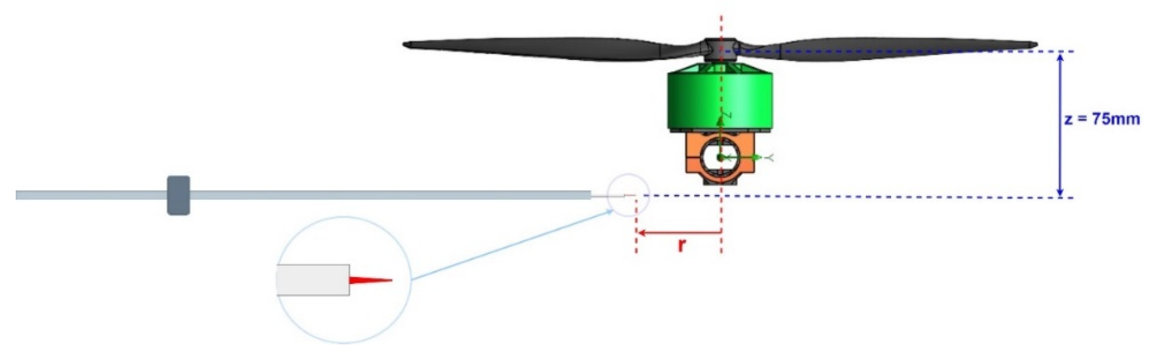
Measurements I—Sensor in the Direction Perpendicular to the Arm and the Propeller Axis at a Distance of 75 mm and r = 0
Regime 60%Regime 70%
Drones 07 00199 i001Drones 07 00199 i002
Regime 80%Regime 90%
Drones 07 00199 i003Drones 07 00199 i004
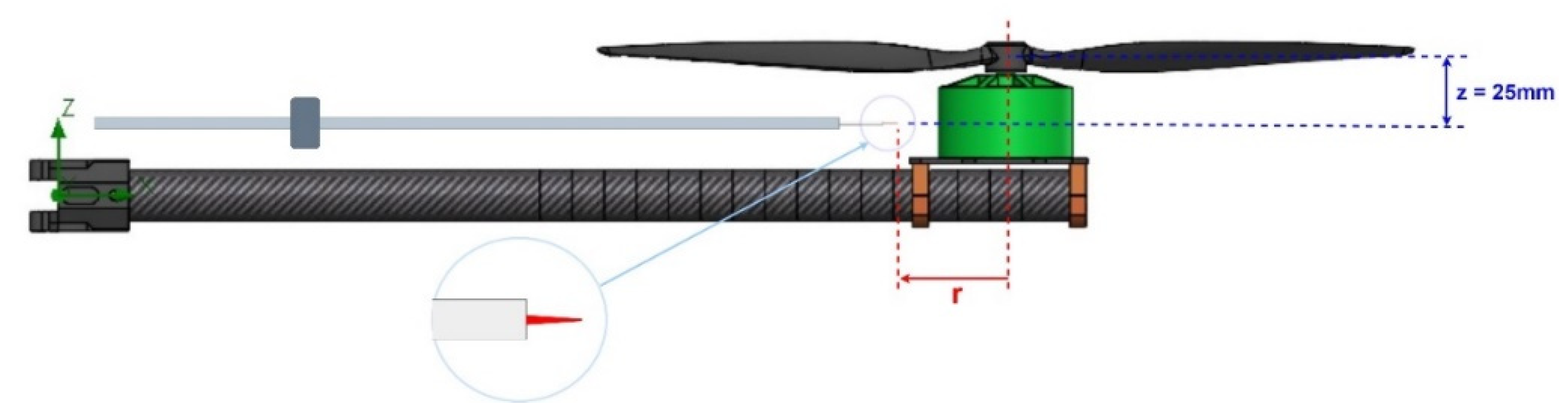
Measurements II—Sensor parallel to the arm at a distance of 25 mm from the plane of the propeller and r = 25 mm
Regime 60%Regime 70%
Drones 07 00199 i005Drones 07 00199 i006
Regime 80%Regime 90%
Drones 07 00199 i007Drones 07 00199 i008
Table 3. Equivalence between the experimental measurement points regarding the velocity components and the recording points of the velocity components from the numerical flow simulations.
Experimental Measurements for Positions I and IIThe Distance r Relative to the Helix Origin for the Measurement PointThe Relative Distance r/Rp
(Rp—Propeller Radius)
Equivalent Point from Numerical Analysis
Measurements I—sensor in the direction perpendicular to the arm in the position 0 degrees at the height z = 75 mmr = 00PG Velocity (Z) 4
r = 200.1574PG Velocity (Z) 8
r = 400.3149PG Velocity (Z) 12
r = 600.4724PG Velocity (Z) 16
r = 800.6299PG Velocity (Z) 20
r = 1000.7874PG Velocity (Z) 24
r = 1200.9448PG Velocity (Z) 28
r = 1401.1024PG Velocity (Z) 32
Measurements II—sensor on the direction along the arm in the position 0 degrees at the height z = 25 mmr = 250.1968PG Velocity (Z) 36
r = 350.2756PG Velocity (Z) 40
r = 450.3543PG Velocity (Z) 44
r = 550.4331PG Velocity (Z) 48
r = 650.5118PG Velocity (Z) 52
r = 750.5905PG Velocity (Z) 56
r = 850.6693PG Velocity (Z) 60
r = 950.7480PG Velocity (Z) 64
r = 1050.8268PG Velocity (Z) 68
r = 1150.9055PG Velocity (Z) 72
r = 1250.9843PG Velocity (Z) 76
r = 1351.0630PG Velocity (Z) 80
Table 4. Comparison between the values of the velocity components recorded at points from the experimental measurements with the CTA and the values of the velocity components resulting from the numerical flow analysis.
Experimental Measurements for Positions I and IIThe Relative Distance r/Rp
(Rp—Propeller Radius)
Equivalent Point from Numerical AnalysisEngine Power Cycles [%]Average Velocity Component Measured with Dantec Dynamics CTA [m/s]Average Velocity from Numerical Analysis [m/s]Absolute Percentage Error
[%]
Measurements I—sensor on the direction along the arm in the position 0 degrees at the height z = 75 mm0460%
70%
80%
90%
1.674
4.073
6.736
7.628
1.190
3.594
5.726
7.087
28.91
11.76
14.99
7.09
0.1574860%
70%
80%
90%
2.094
6.498
10.565
12.191
2.159
6.409
10.098
12.596
3.10
1.36
4.42
3.32
0.31491260%
70%
80%
90%
3.700
10.524
16.932
18.706
3.217
9.491
14.984
18.652
13.05
9.81
11.50
0.28
0.47241660%
70%
80%
90%
4.092
11.916
18.932
22.387
3.834
11.316
17.780
22.267
6.30
5.04
6.08
0.54
0.62992060%
70%
80%
90%
4.064
11.692
19.109
22.808
3.817
11.285
17.772
22.233
6.08
3.48
7.00
2.52
0.78742460%
70%
80%
90%
1.645
7.541
11.787
13.896
1.556
4.618
7.509
9.451
5.41
38.76
36.29
31.99
0.94482860%
70%
80%
90%
0.576
1.571
2.926
3.831
0.196
0.598
0.710
0.904
65.97
61.94
75.73
76.40
1.10243260%
70%
80%
90%
0.279
0.556
0.822
1.001
0.353
1.079
1.485
1.890
26.52
94.06
80.66
88.81
Measurements II—sensor on the direction along the arm in the position 0 degrees at the height z = 25 mm0.19683660%
70%
80%
90%
1.098
2.974
5.915
6.670
0.850
2.530
3.959
4.990
22.68
14.92
33.07
25.19
0.27564060%
70%
80%
90%
2.131
6.275
10.059
11.947
1.939
5.711
8.993
11.192
9.01
8.99
10.60
6.32
0.35434460%
70%
80%
90%
2.088
5.807
9.379
11.034
2.128
6.282
9.894
12.326
1.92
8.18
5.49
11.71
0.43314860%
70%
80%
90%
1.985
5.766
9.162
10.536
2.121
6.362
10.030
12.521
6.85
10.34
9.47
18.84
0.51185260%
70%
80%
90%
2.277
6.647
10.851
12.823
2.363
6.962
10.960
13.685
3.78
4.74
1.00
6.72
0.59055660%
70%
80%
90%
2.519
7.475
12.190
14.606
2.550
7.501
11.792
14.721
1.15
0.33
3.26
0.78
0.66936060%
70%
80%
90%
2.941
8.984
14.482
17.215
2.980
8.823
13.915
17.343
1.33
1.79
3.92
0.74
0.74806460%
70%
80%
90%
3.190
9.506
15.188
18.223
2.945
8.628
13.519
16.959
7.68
9.24
10.99
6.94
0.82686860%
70%
80%
90%
1.507
5.113
9.254
11.758
1.962
5.648
8.708
11.182
30.19
10.46
5.90
4.90
0.90557260%
70%
80%
90%
0.543
1.330
2.624
3.039
0.760
2.271
3.590
4.704
39.96
70.75
36.81
54.79
0.98437660%
70%
80%
90%
0.356
0.929
1.256
1.523
0.773
2.275
3.628
4.248
117.13
144.89
188.85
178.92
1.06308060%
70%
80%
90%
0.438
0.788
1.439
1.394
0.671
2.076
3.209
4.065
53.20
163.45
123.00
191.61
Disclaimer/Publisher’s Note: The statements, opinions and data contained in all publications are solely those of the individual author(s) and contributor(s) and not of MDPI and/or the editor(s). MDPI and/or the editor(s) disclaim responsibility for any injury to people or property resulting from any ideas, methods, instructions or products referred to in the content.

