1. Introduction
Drones are agile, especially quadrotors; ideally, they should fly as fast as they can for excellent movement advantage, both in manual control and autonomous flight. In recent years, the real-time local trajectory planning method for quadrotors is well understood, together with more accurate location and control algorithms, making autonomous flight develop from theoretical scientific research into real-world applications.
A collision-free and dynamically feasible trajectory is indeed the key to autonomous flight. However, the current method only focuses on safety and feasibility, resulting in overly conservative trajectories generated and wasting the agility of the quadrotors. Aggressive local planning remains a huge challenge, which requires rapidly generating high-quality trajectories with faster speed while maintaining safety and feasibility.
Currently, trajectory planning methods can achieve autonomous flight requirements with a moderate speed in an unknown environment. These methods require lots of computational time for redundant environment representation and optimization to generate absolutely safe but conservative low-speed trajectories, which wastes the agility advantage of quadrotors. Therefore, the gradient-based planning method, which continuously optimizes the initial trajectory by gradient information, has great potential to improve the planning and flight speed and is receiving more and more attention.
Among these, Zhou [
1] decouples the online trajectory planning problem as a front-end kino-dynamic path searching and a back-end trajectory optimization, and in optimization, the initial path is further improved in smoothness and clearance by gradient-based information provided by a pre-built Euclidean signed distance field(ESDF) map. However, as the statistics (EWOK [
2]’s Table 2) state, the ESDF build spends time takes up to about 70% of total local planning time. More unfortunately, as analyzed by Zhou [
3], most of the distance gradient information generated by the current ESDF construction methods [
4,
5] is useless for local planning, which causes extra calculation wastes and conservative planning speed. Another gradient-based local planner [
3] aimed at achieving distance gradient information more efficiently compared the colliding trajectory with a collision-free guiding path found by A* algorithm to formulate the collision term in the penalty function. It provided a new way of thinking about how to obtain the necessary distance gradient information to avoid local obstacles; however, its strategy of generating gradient information was not efficient and required many iterations, resulting in it still taking a long time to plan qualified trajectories, especially in complex environments with dense obstacles. In addition, the fitness cost term introduced by the time reallocation problem made the trajectory too conservative, wasting the quadrotor’s natural agility advantage.
Therefore, in this paper, we propose an aggressive gradient-based local planner called Speed-First, which aims to improve planning speed and flight speed under safe and executable conditions. Firstly, a more efficient gradient information generation strategy is proposed, which finds a free-collision Hybrid A* path to replace the collision control points and generates a distance gradient. Secondly, a novel time span cost is presented to aggressively tackle the unfeasible problem and improve the overall trajectory speed. In general, our method can rapidly generate trajectories with a faster speed for more aggressive gradient-based trajectory optimization.
The contributions of our work are summarized as follows:
- (1)
A more efficient distance gradient information generation strategy for faster aggressive planning, which takes only a fraction of the time to drive the trajectory out of obstacles.
- (2)
A novel time span cost term in the second optimization to aggressively but rapidly solve the unfeasible problem and improve the overall trajectory speed.
- (3)
Extensive simulation and real-world experiments to validate our proposed method.
Section 1 and
Section 2: Introduction and overview of the related work of aggressive flight planning.
Section 3: The system overview to introduce the process and key of our method.
Section 4: The distance gradient information generation strategy.
Section 5: A novel time span cost design and the back-end optimization.
Section 6 and
Section 7: Experimental verification including simulation and real-world, conclusion about our work.
2. Related Work
2.1. Quadrotor Trajectory Planning
Trajectory planning for Quadrotors is a key part of achieving autonomous flight. Currently, trajectory planning methods are widely studied and broadly divided into hard-constrained methods and gradient-based optimization methods.
Mellinger [
6] innovatively generated piecewise polynomial trajectories into minimum-snap trajectories through quadratic programming (QP). Richter [
7] further proposed a closed-form solution to minimum-snap trajectories. Gao [
8] generated a flight corridor for the quadrotor to travel through by inflating the path against the environment. Hard constraint methods have evolved to generate trajectories in a two-step pipeline, which searches out initial paths in safe regions and continues to optimize for smooth and feasible final trajectories. The methods rely excessively on the selection of initial paths. On the one hand, the quality of initial paths determines the time for optimization in the back end, and on the other hand, an unreasonable time allocation of piecewise polynomials often leads to unsatisfactory results, which may violate the quadrotor’s dynamics.
As mentioned earlier, the other classical gradient-based trajectory optimization method has received increasing attention because of its high planning success rate and fast planning speed and is becoming the mainstream for UAV local trajectory generation. It formulates the trajectory planning problem as unconstrained nonlinear optimization and utilizes trajectory smoothness and clearance with sufficient gradient information; achieving the gradient information is the key to the problem. General methods rely on a pre-built ESDF map to evaluate the gradient magnitude and direction. ESDF was first introduced in robotic motion planning by Ratliff [
9], which presented a novel method for continuous path refinement that used covariant gradient techniques to improve the quality of sampled trajectories. Oleynikova [
10] presented a continuous-time trajectory optimization method for real-time collision avoidance, which ran at a high rate to continuously recompute safe trajectories as the robot gained information about its environment. Although [
10] slightly relieved the typical local minima by random optimization restarts, it still suffered from a relatively low planning success rate. Usenko [
1] represented the trajectories by using uniform B-splines, which ensured that the trajectory was sufficiently smooth and simultaneously allowed for efficient optimization. To increase the success rate of planning, Gao [
11] found a high-quality collision-free initial path as the front-end and improved the quality of trajectory when kinodynamic constraints [
1] were taken into account. The above work used ESDF to obtain the gradient magnitude and direction needed for keeping a safe distance from nearby obstacles; however, ESDF is expensive and costs a lot of computational resources to achieve mostly useless global gradient information about the environment. Therefore, faster planning speed and how to represent gradient information instead of ESDF is critical to improving planning efficiency.
Zhou [
3] presented an ESDF-Free gradient-based local planner. The planner compared the colliding trajectory with a collision-free guiding path to formulate the collision cost in the penalty function and generated gradient information to wrap the trajectory out of the way of obstacles. After rebounding a few times around local obstacles, the trajectory was absolutely safe in the free region; however, this method still had many disadvantages. On the one hand, the incomplete gradient information generation strategy made the initial trajectory need more optimization iterations to generate an executable trajectory, which wastes a lot of planning time. On the other hand, the fitness cost term introduced to optimize the infeasibility of the trajectory made the whole trajectory too conservative and wastes the agility of the quadrotor. In addition, the fitness cost term changed the size of the trajectory, which required repeated obstacle checks and optimizations for safety that increased precious planning time.
In this paper, we propose a more well-established method to address the above problems. A higher-quality guide path is generated by the Hybrid-A* instead of A* algorithm, considering the dynamic constraints of the quadrotor. The control points trapped in the obstacles in the original trajectory are replaced by collision-free and dynamic guide path points, thereby reducing the optimization pressure and effectively improving the planning speed. In addition, the time span cost term is innovatively proposed. On the one hand, the infeasibility of the trajectory is solved without compromising the trajectory’s aggression. On the other hand, it brings the time span of the trajectory represented by the uniform B-spline closer to the limit, which lifts the whole speed of the trajectory.
2.2. Aggressive Flight in Unknown Environments
Achieving onboard high-speed flight or generating a more aggressive trajectory requires efficient planning speed and ultimate flight speed under feasibility conditions.
Specifically, a widely accepted idea is that the quadrotor can replan new trajectories to avoid unexpected obstacles in a very short reaction time. The typical work represented by Zhou [
12] finds a locally optimal trajectory confined within a topologically equivalent class by capturing a collection of distinct useful paths in 3D environments. Although increasing the planning success rate and speed, it does not necessarily contain a satisfactory solution for smooth and safe navigation, especially on the fast flight. Ref. [
13] presents a new idea to solve the problem of sudden obstacles that appear during the movement due to the limitation of the field of view(FOV) and failure to replan. It introduces a perception-aware planning strategy to observe the local environment and avoid unknown obstacles in advance. The risk-aware trajectory refinement ensures that unknown obstacles which may endanger the quadrotor can be observed earlier and avoided in time. However, perception-aware planning causes the trajectory to become relatively conservative, making the trajectory lengthy and the flight speed slower.
Recent work [
14] has demonstrated a stunning achievement of high-speed flight in an unknown environment using a receding flight corridor. In particular, it generated the safe receding horizon flight corridor rapidly by using a 3D Gaussian distribution sampler and tested up to 13.8 m/s in an unknown environment. However, the Gaussian distribution sampler method is tricky, and the empirical parameter settings make the method unsuitable for any scenario, which means it has a non-negligible risk in corner cases. In addition, the bottom line is that excellent real-world flight may depend more on the effectiveness of costly, but fast, instant LiDAR map building, and the role of planning is relatively less important in the realization of high-speed flight.
Ref. [
15] proposes an innovative solution to solve autonomous fast flight in an unknown environment. It argues that the traditional pipeline solution divides the implementation of autonomous flight into sensing, mapping, and planning, which leads to increased processing latency and compounding of errors. Therefore, it presents an end-to-end approach that directly maps noisy sensory observations to collision-free trajectories and furthermore, performs the sensorimotor mapping by a convolutional network. In the end, it achieves zero-shot transfer from simulation to the real world. Unfortunately, although it runs high-speed autonomous flight in a cluttered outdoor environment, instability due to dependence on training data quality and size potentially limits the real application of this work.
In this paper, we still stand for a traditional pipeline solution and focus on improving the efficiency of the planning module compared to the classical gradient-based local planning method [
3]. The speed of the whole trajectory will be improved at the limit by a fresh span time cost term based on safety, smoothness, and feasibility.
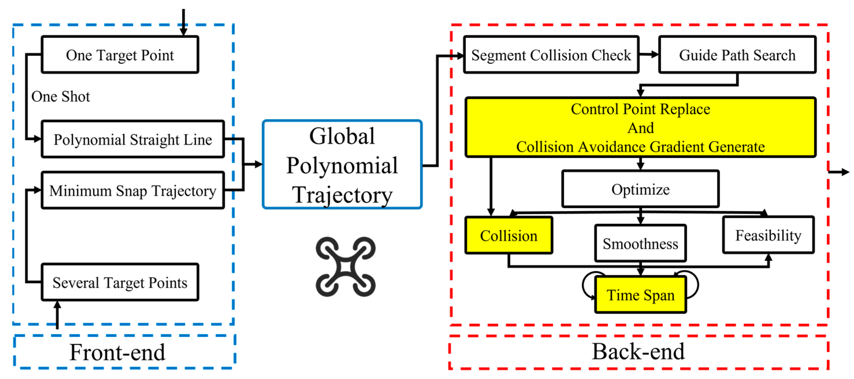
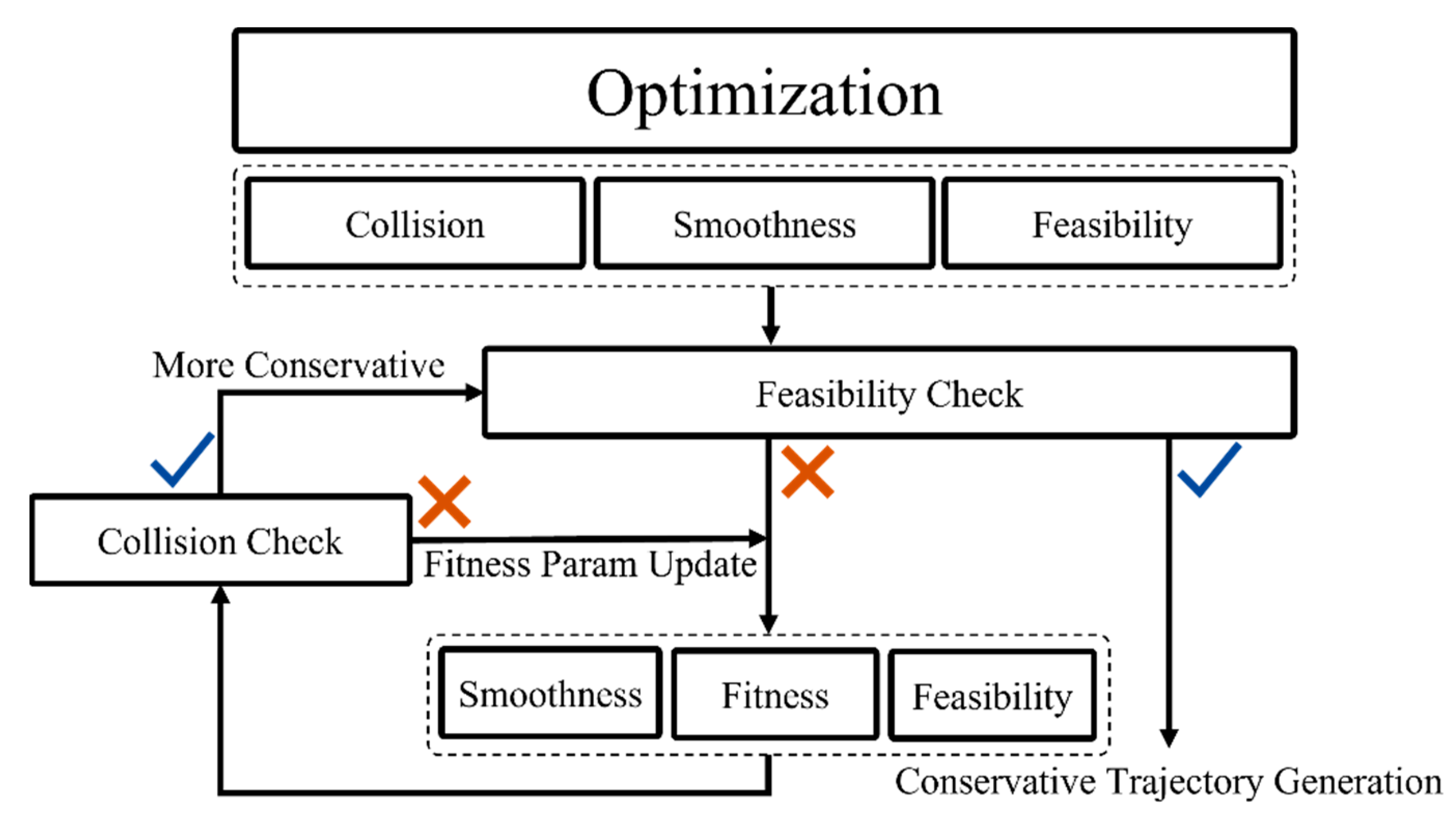
3. System Overview
In this article, as shown in
Figure 1, we follow a two-step trajectory planning framework similar to [
3], which plans an initial global polynomial trajectory in the front end and optimized the local trajectories based on local environment information in the back end.
In the front end, when the number of target points is unique, we use a one-shot strategy to represent the global trajectory directly with a polynomial straight line (smoothly changing velocity and constant acceleration) to ensure it is the shortest. When there are several target points arriving in a certain order, we generate a minimum snap trajectory [
6] as the global trajectory to smoothly connect the target points. In the front end, the generated global polynomial trajectory ignores the environmental information.
In the back end, we check the global trajectory collisions segment by segment only in the local environment within the sensor range. A local guide path is searched by Hybird-A* when collisions occur. We replace the control points in obstacles with responding guide path points and generate collision avoidance gradient information, including magnitude and direction. Trajectory optimization is divided into two stages. In the first stage, the initial trajectory is optimized for safety, smoothness, and feasibility to rapidly generate a high-quality trajectory. The fresh time span cost term is added to continuously optimize the previous trajectory. The shape and size of the trajectory represented by uniform B-splines do not change with the time span. Therefore, a more aggressive trajectory is generated that guarantees safety, smoothness, and feasibility.
4. Distance Gradient Information Generation
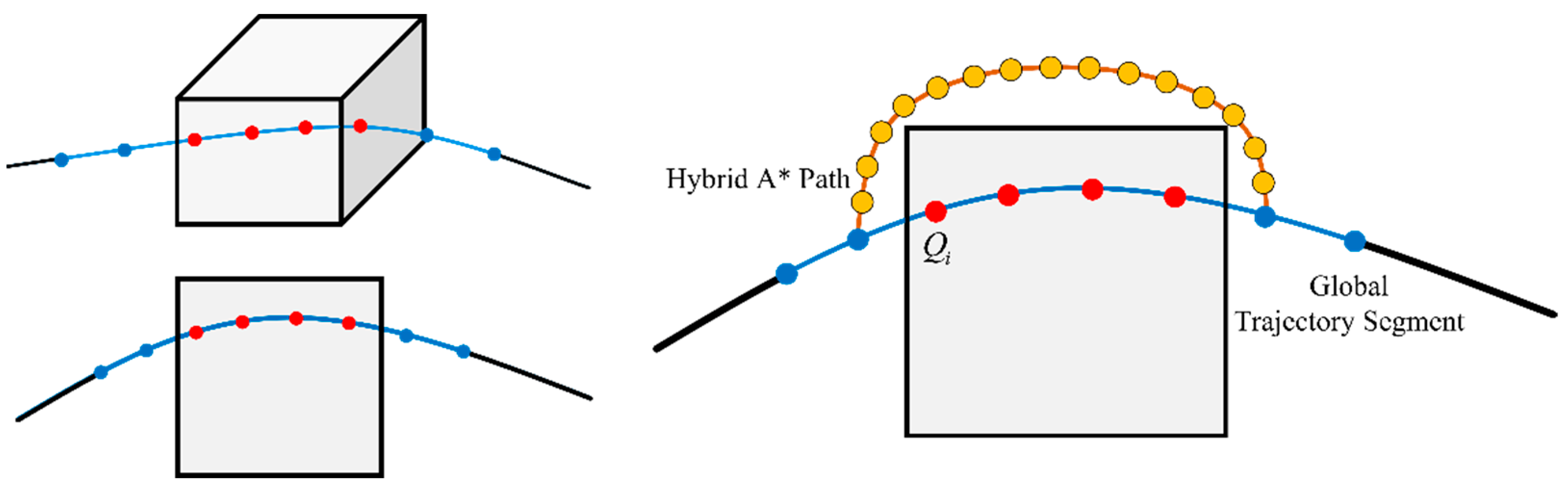
4.1. Control Point Replacement
The essence of the B-spline curve is a parametric polynomial obtained by fitting the control points and knot span
. In the front-end, we have obtained a global polynomial trajectory ignoring environment obstacles that connect the start and target points, which is essentially a B-spline curve that satisfies the terminal constraint. Each segment is checked in an iteration of whether in obstacle. When the collision occurs, a collision-free Hybrid A* path is generated. Hybrid-A* algorithm [
16] was first used to generate smooth paths for an autonomous vehicle. Here we apply it to find a smooth but close to obstacles guide path for replacing collision-free control points and generating high-quality distance gradient information.
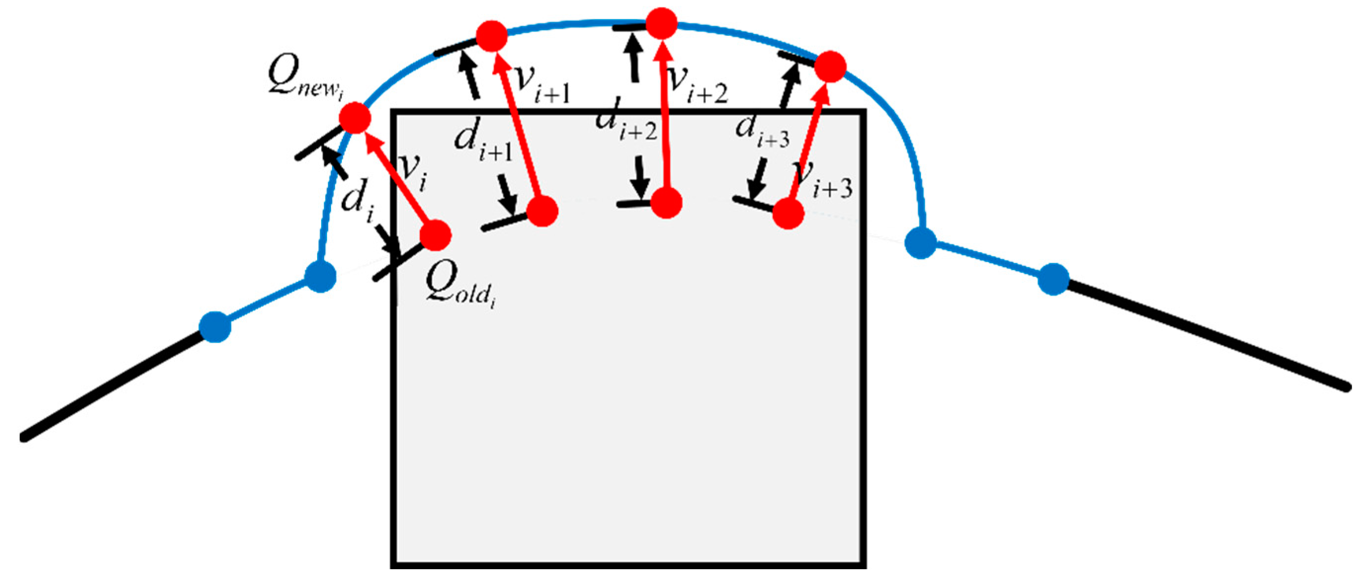
As shown in
Figure 2, when several control points
are in obstacle, a Hybrid-A* path will be generated as a guide collision-free path starting from the last control point that does not enter the obstacle and ending at the first control point that leaves the obstacle. In [
3], as compared in
Figure 3, when collisions occur, the guide path is generated by A* algorithm, which generates low-quality gradients in an unsmooth shape and results in more iterations for back-end optimization. This issue will be mentioned in detail in
Section 4.2.
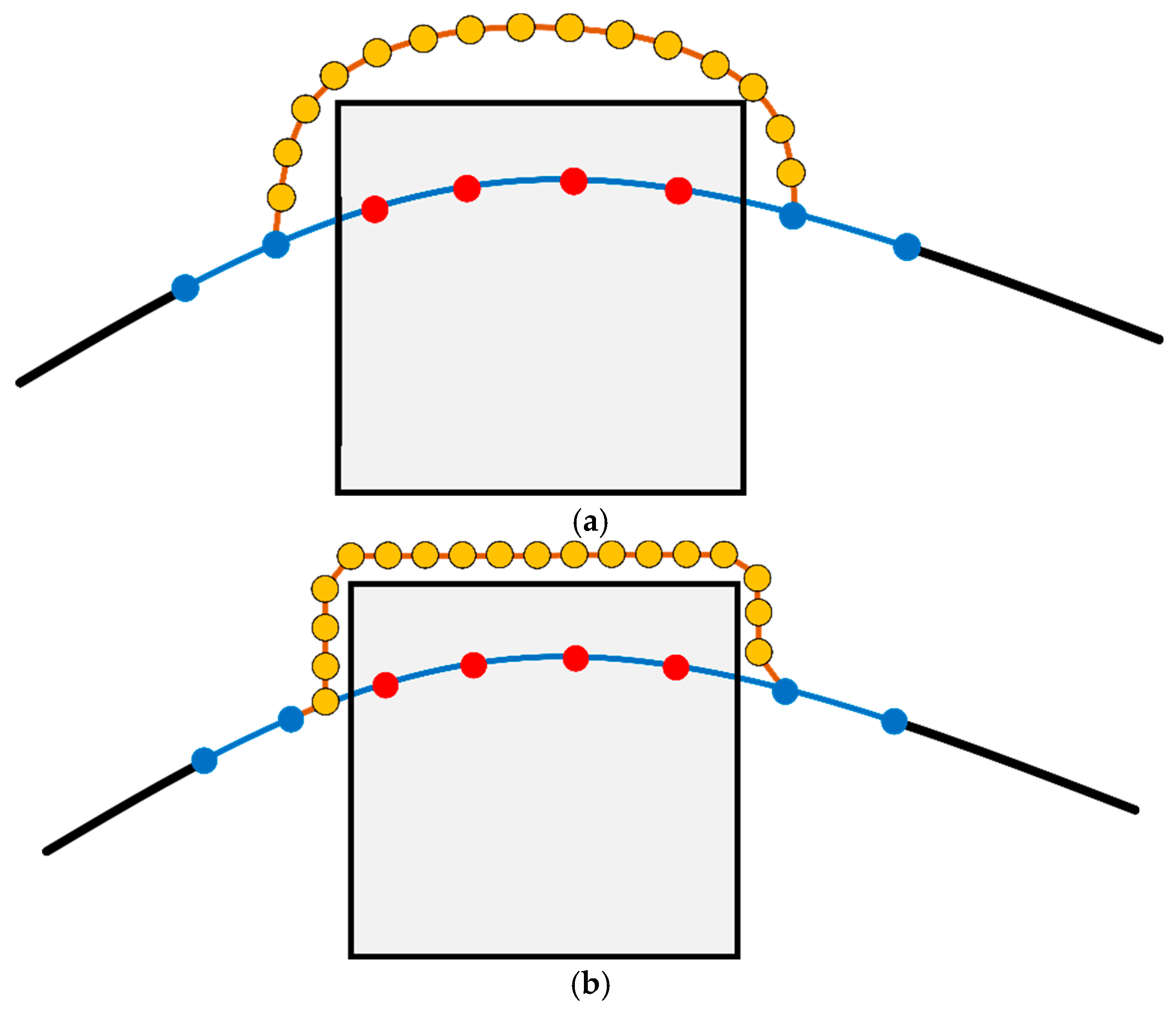
After achieving the absolute collision-free guide path, we adopt a replacement strategy, which replaces the corresponding guide path points with the original control points in the obstacle according to the serial number.
Figure 4 shows the specific method for control point replacement. The guide points are evenly divided according to the number of control points in the obstacle. Then corresponding guide points replace them as the new correct sequence of control points.
The newly generated B-spline curve is already collision-free, but it is too close to the obstacle, which is a higher threat to the safety of the quadrotor. Therefore, it is absolutely necessary to use the distance gradient information to optimize the current trajectory and improve its smoothness and clearance. We will present in the next section how to define the gradient information from the refined new control points and the corresponding old control points instead of using a pre-build ESDF map.
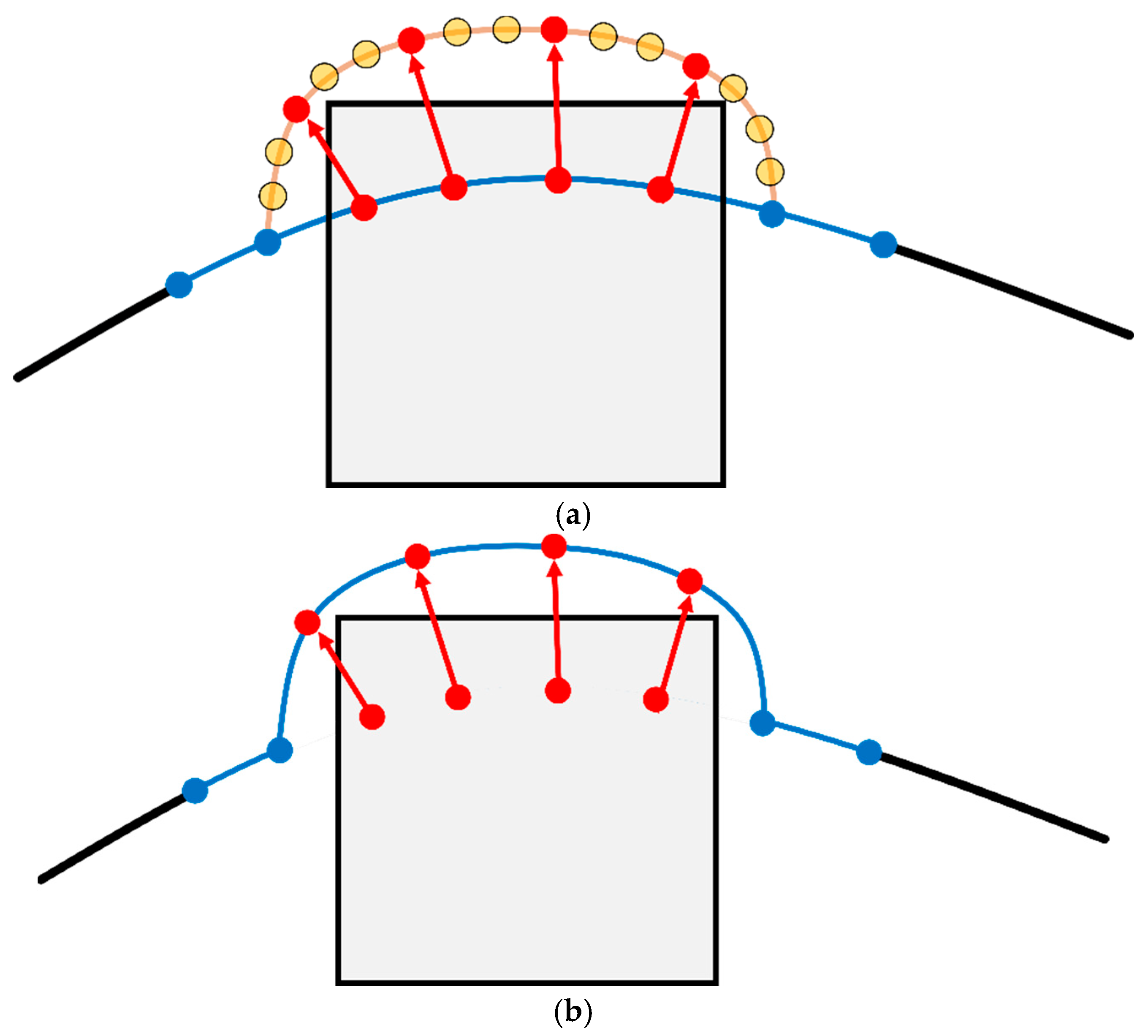
4.2. Collision Avoidance Gradient Generation
We have gained the information about new refined control points and the corresponding old control points in order, which can be seen as a pair of repulsive point sets. The old control points
are considered as repulsion source, which generates a repulsive field that only pushes outwards towards the corresponding new control points
, which is inspired by the artificial potential field method proposed by Khatib [
17].
The collision avoidance gradient for collision optimization contains the gradient magnitude and direction. As shown in
Figure 5, the Euclidean distance
of between
and
is estimated to express the gradient magnitude, and the vector
is used to indicate the gradient direction.
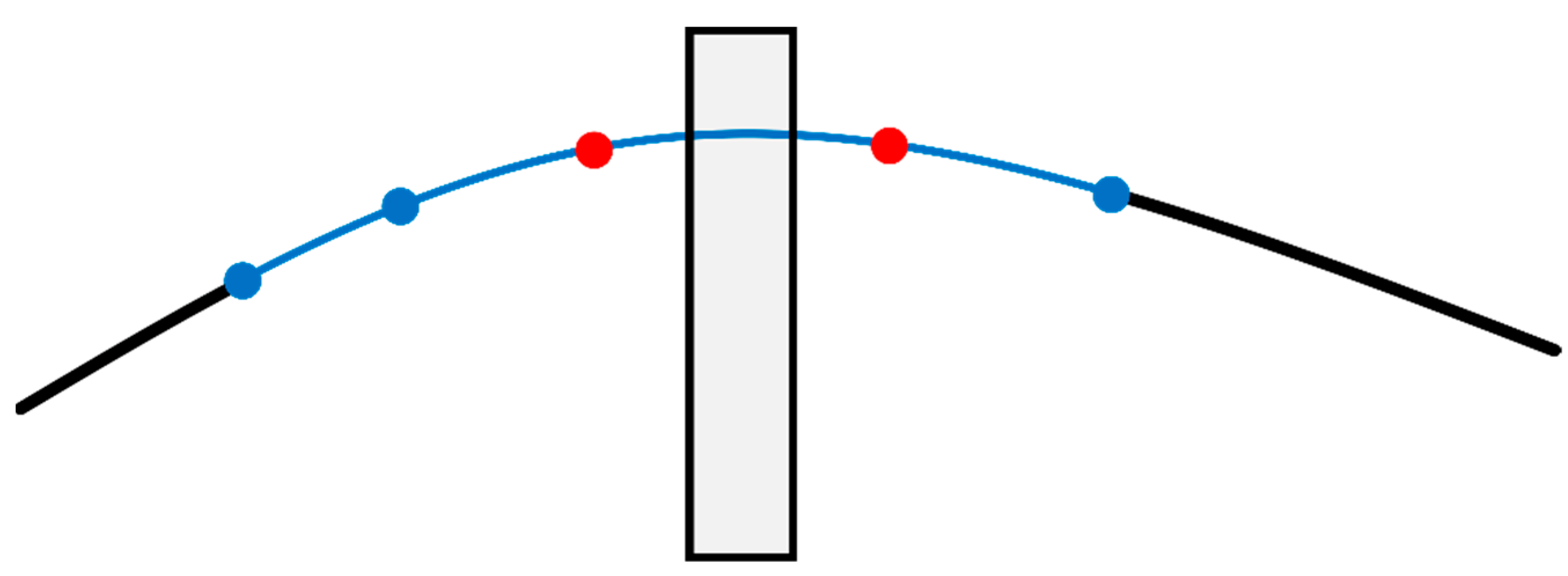
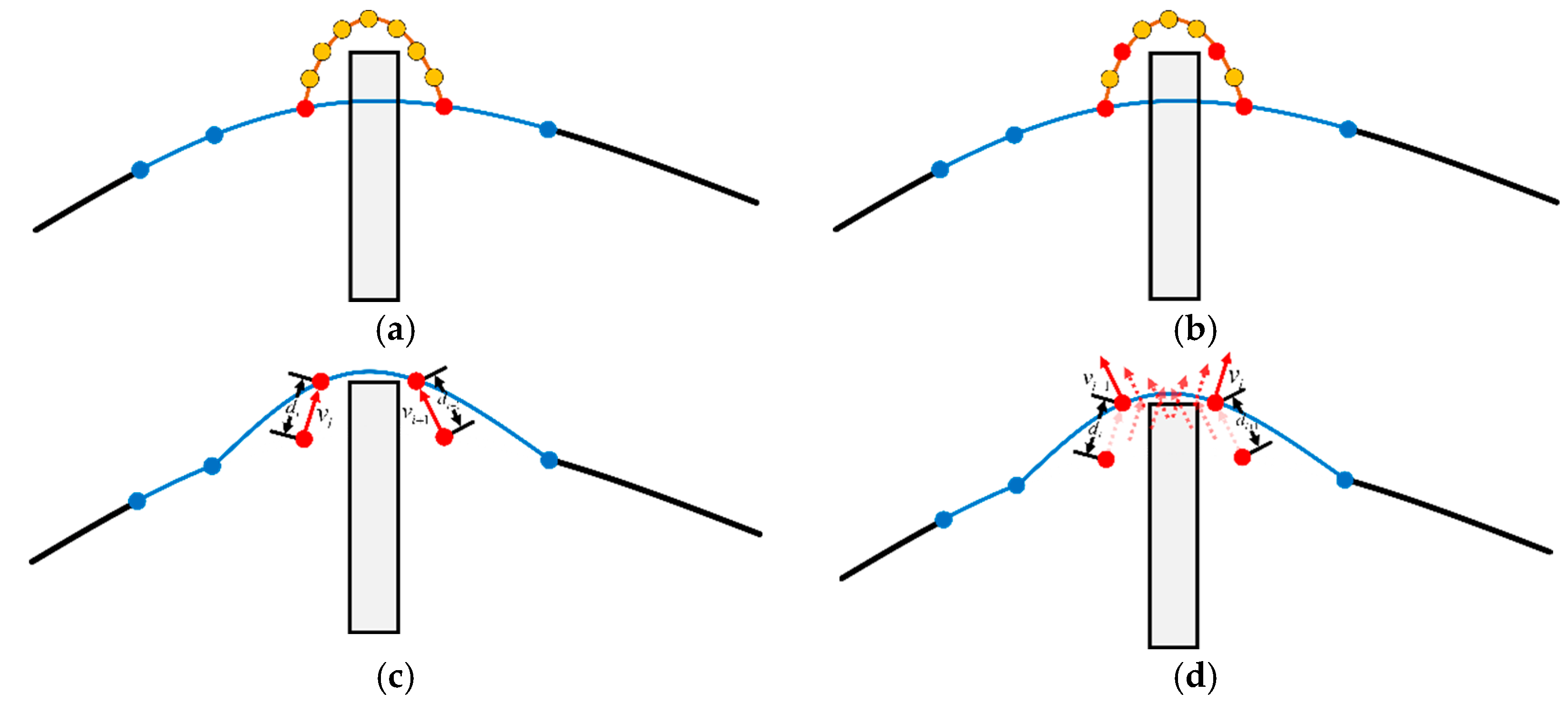
Additional attention is required for a special case shown in
Figure 6, which means the obstacle is too thin to cover the control points of the initial global trajectory. In the thin case, a guide Hybrid-A* path is generated in the same way as
Section 4.1 mentioned. The guide path points will be divided into three to take the middle two points as refined new control points.
As shown in
Figure 7, after the initial definition of collision avoidance force, the gradient direction is swapped to ensure that the new control points close to the obstacle are pushed correctly away from the obstacle.
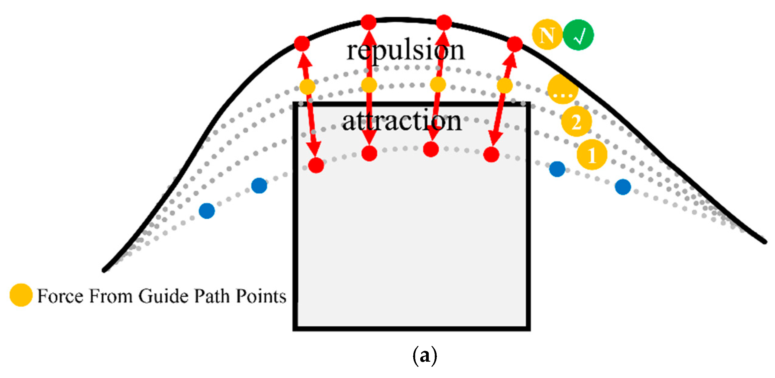
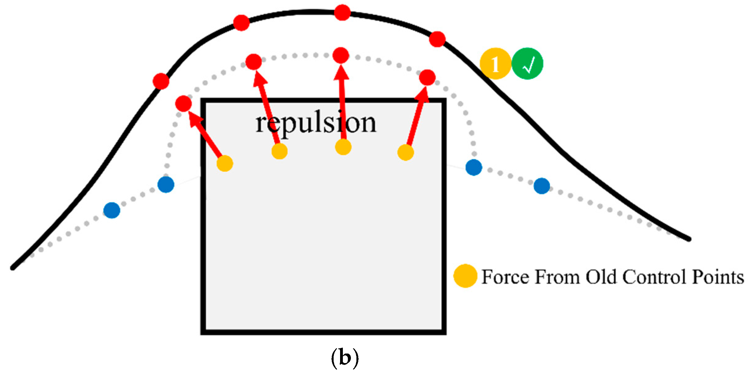
Compared to [
3], which projects the gradients onto the colliding control points and generates an estimated gradient with an A* guide path to wrap them out of obstacles, the method we upgraded effectively increases planning speed. As shown in
Figure 8, in the original work [
3], guide A* path points were used as the power source. The power attracted the global trajectory to pull it out of the obstacle when the global path was trapped in the obstacle, and then converted to repulsive force to push it away to a safe distance. This process often takes several iterations, which include a shift in gradient direction that is detrimental to the optimization. Therefore, we creatively used the Hybrid-A* algorithm to find a dynamic guidance path and control points replacement strategy to optimize the redefined and absolutely safe trajectory with higher-quality gradient information. The planning speed was improved for more optimization-friendly gradient information and fewer iterations. We verified the effectiveness of the method in our experiments, as shown in
Section 5.
5. Time Span Optimization for Faster Flight
As mentioned earlier, current methods are overly conservative and waste the agile nature of drones. Undoubtedly, we need to set the dynamic limits , according to the actual motion ability of the drone. A high-quality trajectory that can be executed realistically must meet the dynamic feasibility, which requires that the speed and acceleration of the entire trajectory do not exceed the limits , set in advance. However, current methods over-optimize the feasibility cost to generate a conservative trajectory which loses the agility of the quadrotor.
Therefore, in this section, we divide trajectory optimization into two stages. In the first stage, the initial trajectory is optimized for safety, smoothness, and feasibility. And a time span cost term is proposed to increase the speed of the entire trajectory under dynamic limits to make it as close to the maximum speed as possible.
5.1. Problem Formulation
A B-spline is a piecewise polynomial uniquely determined by its degree , a set of control points , and a knot vector , in which , , and . A B-spline trajectory is parameterized by time , where . For a uniform B-spline, each knot has the same value . This is the basic principle of the B-spline representing polynomial trajectories.
In our work, the trajectory is parameterized by a uniform B-spline curve, which represents each knot is separated by the same time span. The problem formulation is based on the classic quadrotor local planning framework [
1], which divides the trajectory into three categories of indicators for optimization.
5.2. First Optimization
The optimization problem in the first stage is formulated as follows:
where
,
are smoothness, collision, and feasibility costs.
,
are the weights for each cost term.
- (1)
Smoothness cost
In previous work [
2], the smoothness cost is formalized as the time integral over square derivatives (acceleration, jerk, and snap) of the trajectory, which increases the complexity of the solution. In the framework [
1], only geometric information is considered, but the time span is ignored. Therefore, we follow the smoothness cost designed by [
3], which considers the time span to generate higher-order information on the trajectory.
An elastic band cost function inspired by [
18,
19] is used to define the smoothness cost
:
where is the velocity
calculated by adjacent control points. The cost function consists of the acceleration
and the jerk
between adjacent control points
,
, and
, which captures the geometric information of the trajectory and carefully considers the time span
. Benefiting from the convex hull property, it is sufficient to reduce these derivatives along the whole curve by minimizing the control points of higher-order derivatives of the B-spline trajectory. A more smooth trajectory is obtained by minimizing
, which is more friendly to the execution of the trajectory.
- (2)
Collision cost
In [
3], an unreasonable definition of gradient magnitude complicates the estimation of avoidance force, in which the distance value used for cost calculation may be negative. So in our work, as described in the previous section, the distance value is strictly limited to the positive value range by the control point redefinition strategy, so the calculation of the collision term is simplified. The Euclidean distance
between
and
is estimated to express the gradient magnitude.
Therefore, the collision cost function is formulated as:
where
is the safe distance set in advance, and
is the collision cost for each control point. A twice continuously differentiable cost function is made to further facilitate optimization.
- (3)
Feasibility cost
As the quadrotor dynamics are differentially flat [
6], we can ensure feasibility by restricting the higher-order derivatives of the trajectory on every single dimension. And it’s sufficient for constraining derivatives of the control points to constrain the whole trajectory thanks to the convex hull property of the B-spline. We follow the method [
3] to design the feasibility cost, and the cost function is formulated as:
where
,
,
are weights for each term.
is a twice continuously differentiable metric function of higher-order derivatives of control points and is composed as follows:
where
. And
is further designed as:
where
,
,
,
,
,
are the parameters set for the second-order continuity,
is the limit of derivative, and
is the splitting points of the quadratic interval and the cubic interval.
is the flexible elastic coefficient ranging 0–1 to make the final results meet the constraints.
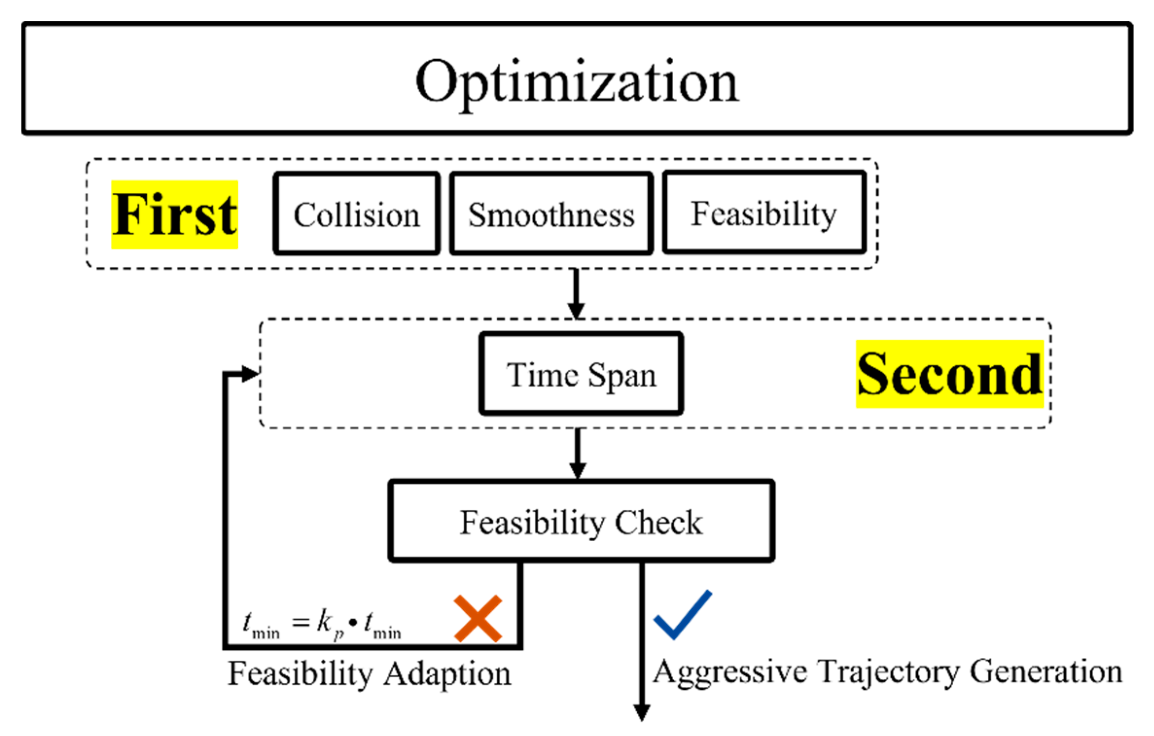
5.3. Time Span Second Optimization
As mentioned before, suffering from the conservative trajectory planning, the quadrotor can fly at low speed in the environment resulting in the waste of agility. Therefore, in this section, we propose a fresh time span optimization cost term that innovatively considers the time span into the secondary optimization.
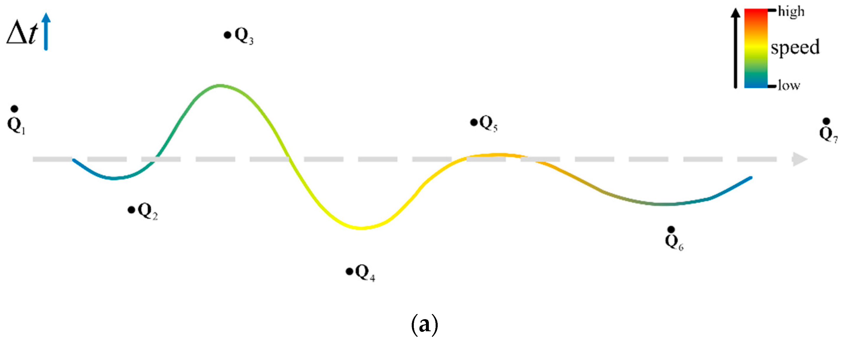
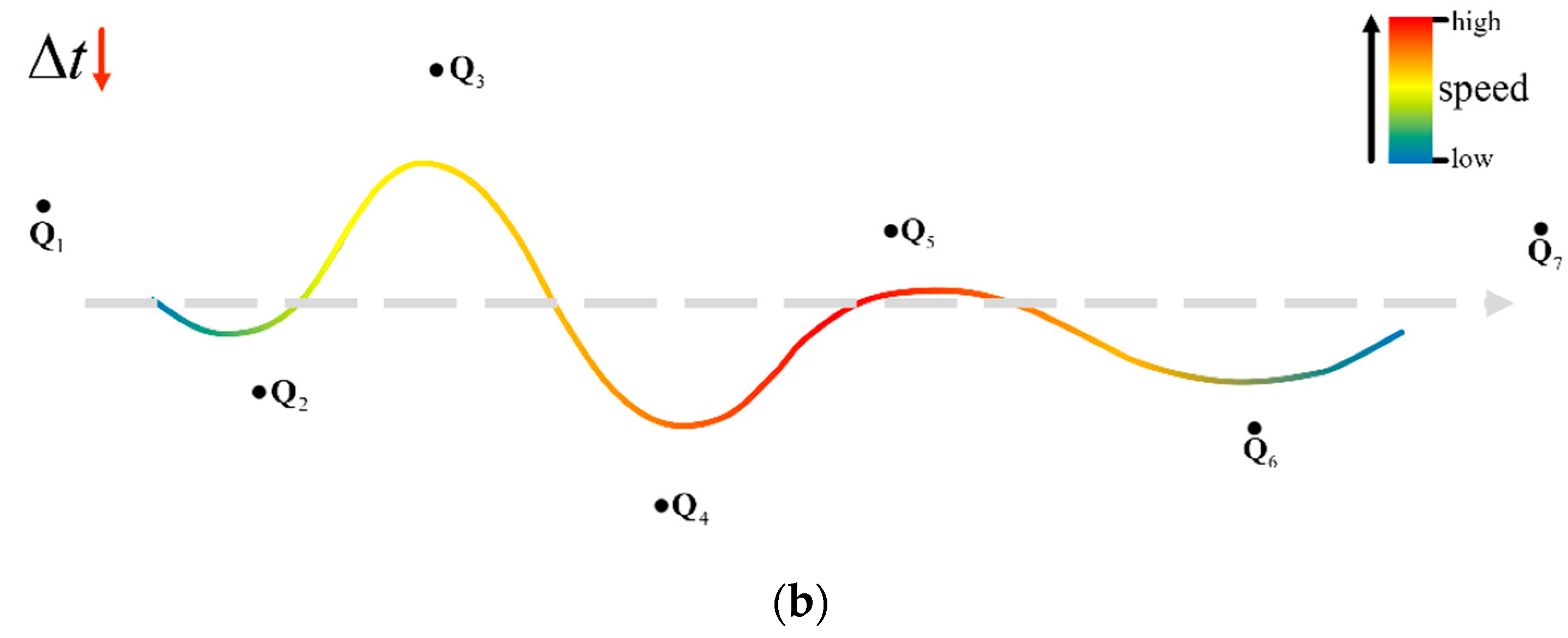
Unlike Bezier curves, the value of
in B-spline is not limited to [0, 1]. For a uniform B-spline curve that has the same distance between two control points, expanding
does not change the spatial shape of the B-spline curve but influences the speed (velocity and acceleration) of the whole trajectory, which shows in
Figure 9.
Therefore, after the first optimization has determined the curve spatial property, the trajectory is continued to be optimized for faster flight under the dynamic limit without worrying about collisions due to the secondary optimization. In the previous section, a smooth, safe, but conservative trajectory has been generated by the first optimization which has ensured the specific position for each control point . Based on this trajectory, a time span cost term is designed to make the speed closer to the limit for an aggressive motion.
Thanks to the fixed position of the control points after the first optimization, the minimum span time
can be calculated by the distance between two adjacent control points
,
and the limit velocity
:
The time span cost function is formulated as:
is used for the second stage optimization and the trajectory will be checked for feasibility.
is a gain factor. If there is a speed or acceleration beyond the limits
,
, an iteration of the secondary optimization will yield, which carefully increases the minimum span time
by a scale factor
.
Figure 10 shows the process of optimization more clearly.
In the first stage of optimization, the initialized global trajectory is rapidly optimized to a safe trajectory that basically meets the flight requirements. After this, the second stage continues to optimize the quality of the first stage trajectory (including the overall speed and dynamically feasible improvement) at a negligible time cost in order to achieve a faster generation of more aggressive trajectories compared to the classical gradient-based method [
3]. On the one hand, the creation of the time span optimization cost term simplifies feasibility adaption problem that the trajectory does not strictly meet the feasibility after the gradient optimization of the feasibility cost term, on the other hand, the speed of the whole trajectory is reasonably improved within the allowable range, making the trajectory more aggressive.
However, the method [
3], which is the classical ESDF-free gradient-based optimization method and proposed an anisotropic curve fitting algorithm to adjust higher order derivatives of the trajectory, has a more complicated optimization process shown in
Figure 11.
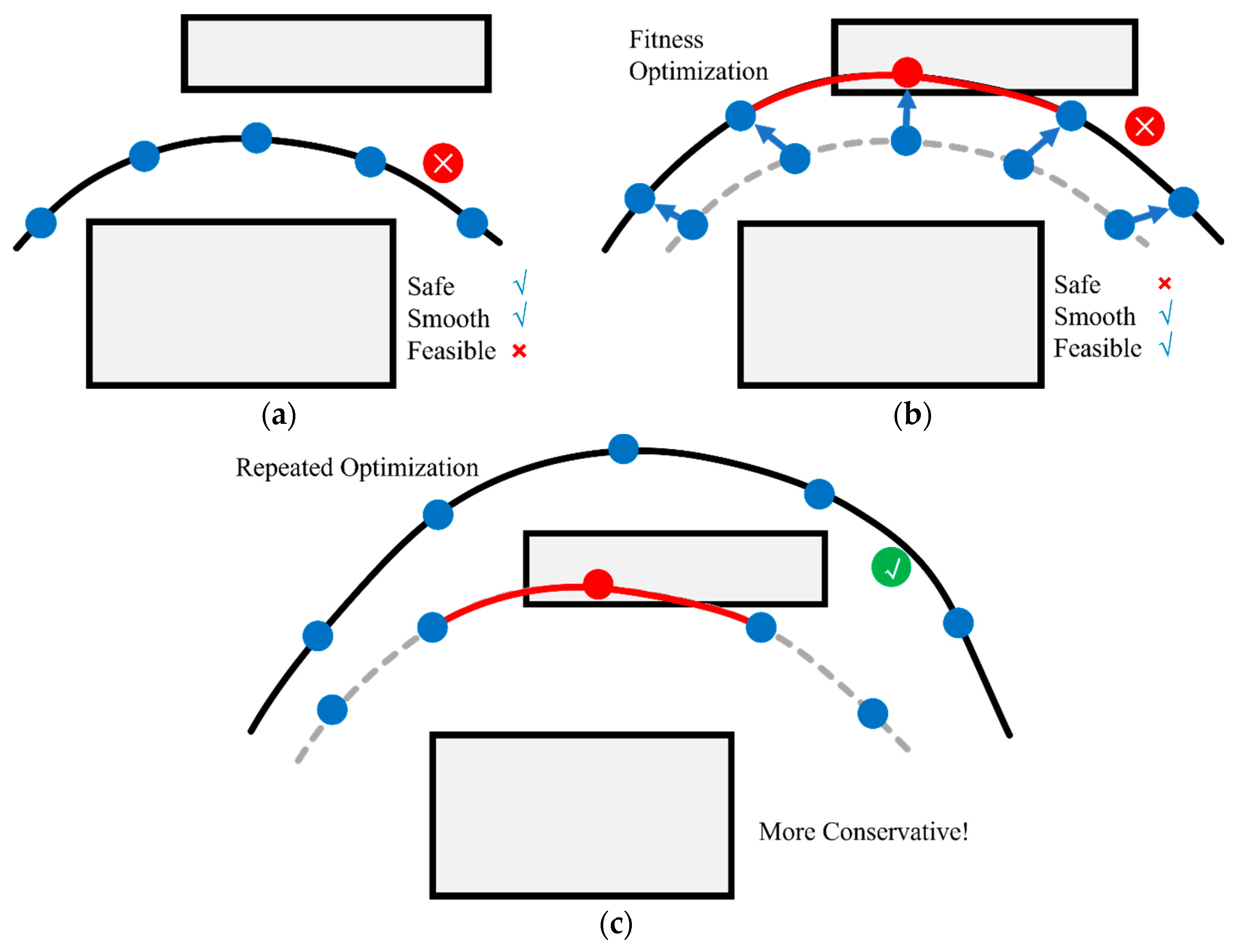
Fitness cost term can solve the problem of infeasible dynamics, but it also has other disadvantages. As shown in
Figure 12, firstly, the fitness cost term
is optimized by combining smoothness and feasibility cost term, which will change the shape and size of the trajectory and may occur a bad new collision resulting in repeated optimization. Secondly, the complicated optimization process increases the planning time and reduces the real-time planning. Thirdly, repeated and conservative optimization leads to a more lengthy trajectory, resulting in longer trajectory length and lower flight speed.
6. Experiment result
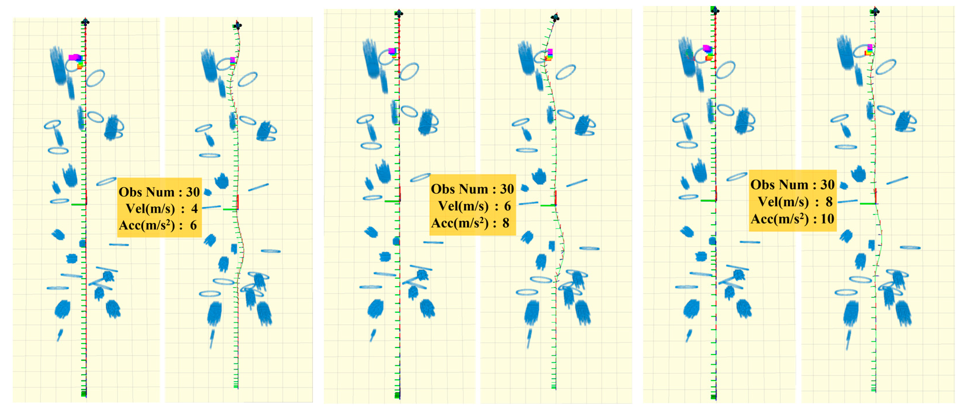
6.1. Simulation and Analysis
We verified our work in simulation and compared it with the classical ESDF-free local planning method Ego-Planner [
3]. Simulation experiments were tested in three 5 × 20 × 3 m
3 complex maps with different obstacle densities, as shown in
Figure 13.
Two methods used almost identical parameters, as shown in
Table 1, differing only in the presence of weighting factors for different optimization terms. The FOVs of the sensors in simulations were set as [80 × 60] deg with a maximum range of 4.5 m.
As shown in
Figure 14,
Figure 15 and
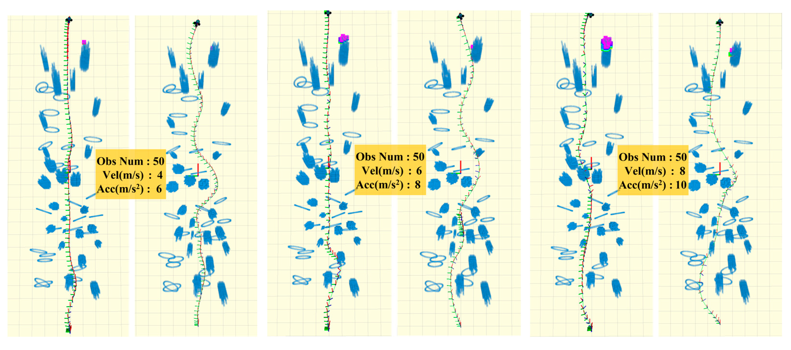
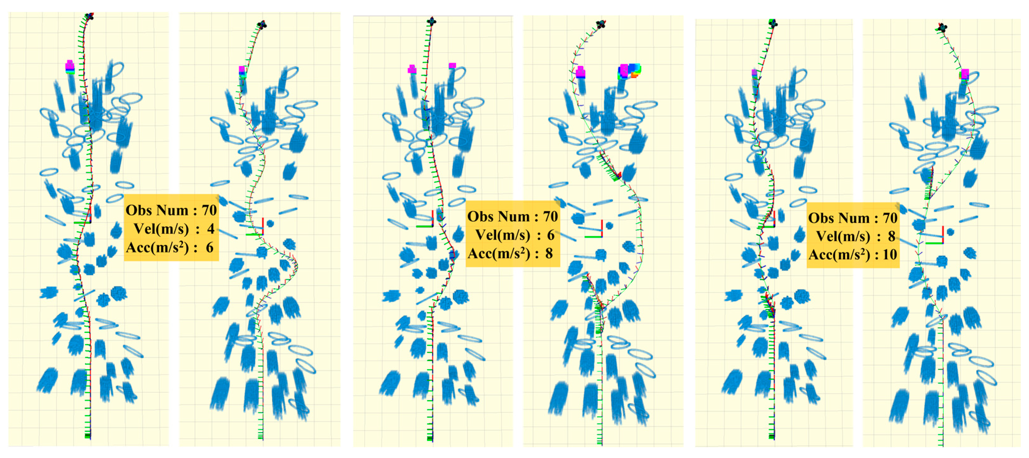
Figure 16, each test had the same start (−12,0,1) and endpoint (12,0,1). The quadrotor was required to avoid obstacles with different densities during flight under dynamic limits we set in advance. Planning time refers to the average time required by the planner to generate a desired local trajectory, which reflects the lightness and planning speed of the methods. Flight time, max flight velocity, and mean flight velocity reflects the higher dimensional velocity information of the desired trajectory and the true speed in execution, which measures the aggressiveness of the methods.
Through the comparison of three sets of simulations, the conclusion can be summed up as follows: (1) relatively straight trajectories were generated by the method we proposed compared to Ego, benefitting from a more flexible gradient information generation strategy and time span cost term instead of repeating optimization. (2) As shown in
Table 2,
Table 3 and
Table 4, the performance (planning and flight speed) of our method was consistently better than Ego under various conditions. (3) The more dense the environment with obstacles, the more obvious were the advantages of our approach. (4) Ego failed to generate a trajectory with conditions: 70 obstacles,
= 8 m/s,
= 10 m/s
2, while our method still generated a safe and executable trajectory in such a harsh environment.
The reasons are analyzed why we can maintain relatively better performance in empty and crowded environments:
When the quadrotor is in a completely empty environment and there are no obstacles around, the collision cost is always 0, but the cost of feasibility will decline if the speed of the whole trajectory becomes smaller. That is why the quadrotor illogically slows down in areas that are almost free of obstacles. Therefore, we proposed the time span cost to ameliorate this unreasonable conservative planning and make the speed increase.
When the quadrotor is in a cluttered and complex environment, the repeated iterative optimization of Ego allows the trajectory to avoid collisions safely and satisfy dynamic feasibility but increases the planning time and makes the trajectory too conservative and lengthy, as we mentioned earlier. However, our method retained the safe but unfeasible trajectory after the initial optimization, and the time span optimization item was used for re-optimization on this basis, which generated a more aggressive trajectory.
The reasons for the stability of the Speed-First are also discussed. First, compared to the classical gradient-based methods, Speed-First can generate trajectories faster and fewer iterations of optimization, which avoids the triggering of safety protection and is the common protection mechanism that directly stops flight behavior due to avoiding unavoidable collisions caused by untimely planning. Besides, the control point replacement method, which uses the collision-free A* guide points to replace the original control points in obstacles, guarantees the success rate of planning as long as there is a feasible space, even if the trajectory is not so perfect (meaning that there is still room to improve the smoothness as well as the feasibility).
6.2. Real-World Tests
To verify the effectiveness of our proposed method in the real world, we conducted extensive real-world experiments in a cluttered outdoor scenario and compared it with Ego [
3].
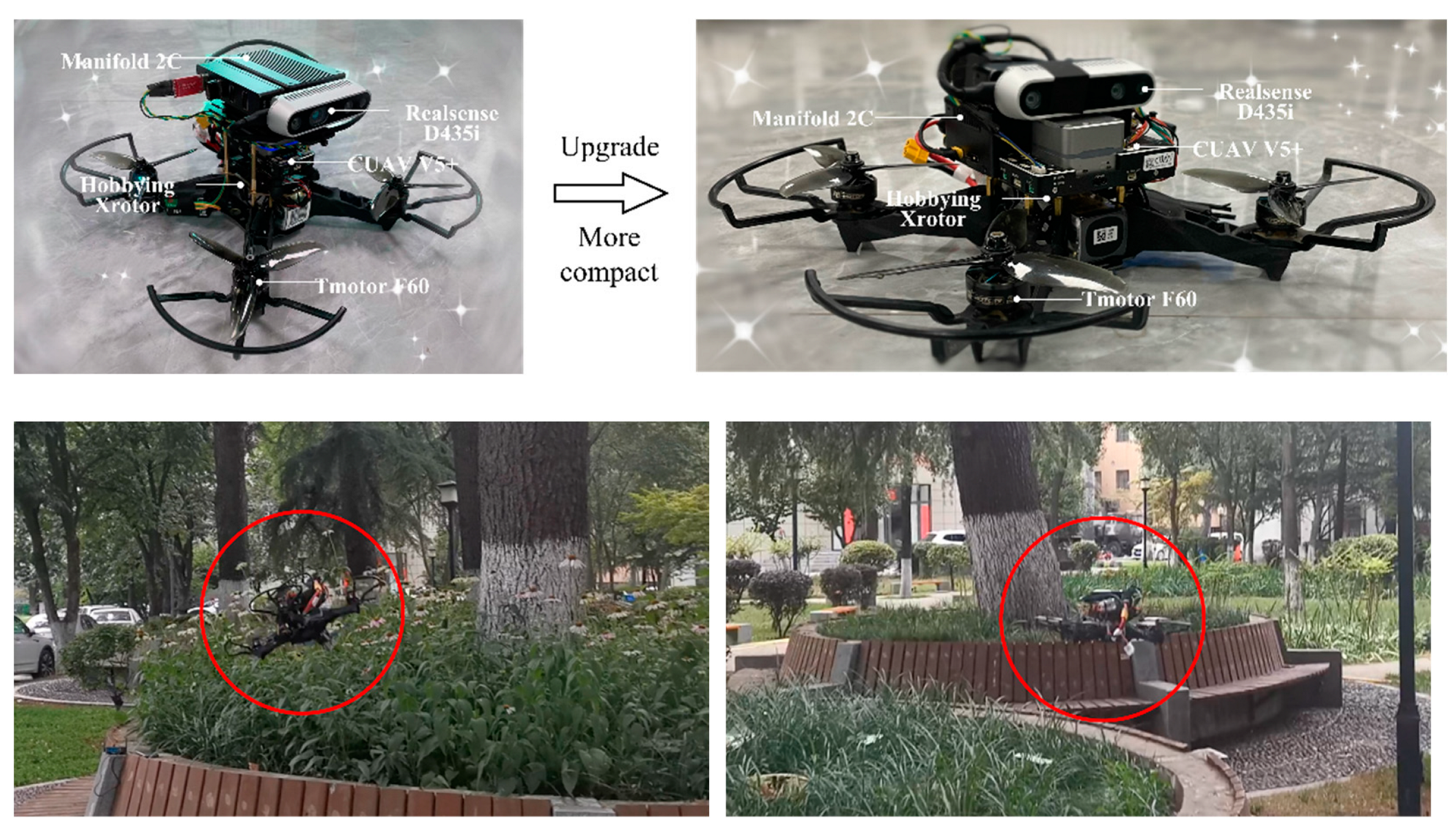
In real-world experiments, a visual-inertial state estimator called VINS-Fusion [
20], which only needs a visual camera and the imu information of the flight controller, was used to provide the necessary localization—a classic controller for quadrotors [
6] to track the trajectories. All experiments were completed by a DIY quadrotor platform. It should be noted that the platform had a great influence on aggressive flight, especially the tracking effect of the trajectory. Therefore, we upgraded our platform, becoming more compact and more advantageous to eliminate the influence of other factors and highlight the effect of planning. The hardware configuration of the platform is shown in
Table 5, and the look and performance in the real world of the compact platform are shown in
Figure 17.
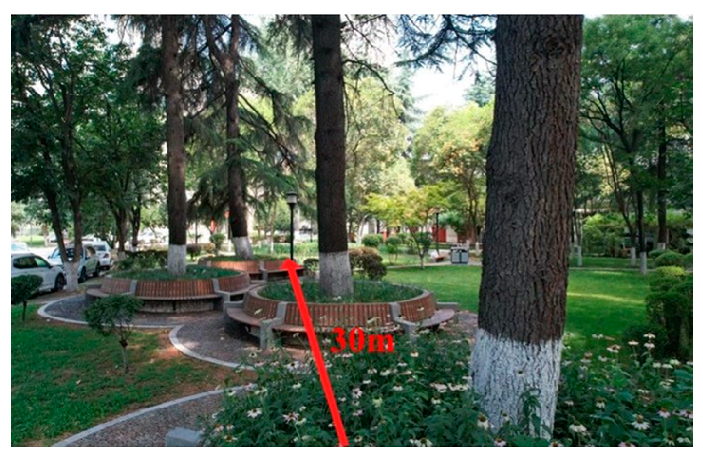
The real-world experiments were tested in a cluttered and messy forest shown in
Figure 18. In each experiment (both ours and Ego [
3]), we required the quadrotor to reach the end point set in advance, which is 30 m away from the start point. And the parameter setting is also following
Table 1.
To verify our method for improving the whole trajectory speed in the real world, a comparison test was conducted under the same dynamic limits
= 2 m/s,
= 3 m/s
2. The performance of two planners is shown in
Figure 19. The specific data are listed in
Table 6. In real-world experiments, our method obtained results similar to those of the simulation, verifying the applicability of our approach. Under the same dynamic limits, the method we proposed can generate more aggressive trajectories while satisfying safety and feasibility. Besides, the planning speed and the overall trajectory speed are improved compared with Ego.
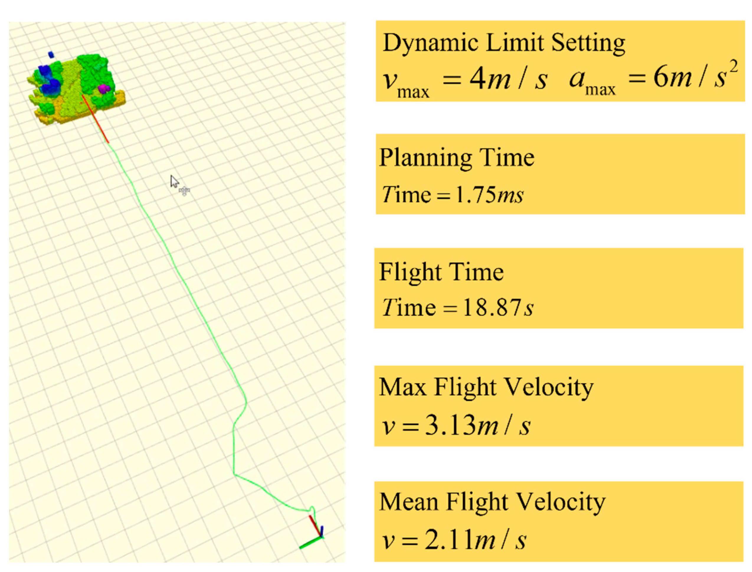
We conducted an extensive experiment to test the extreme flight performance in the real world, which is unavoidably affected by platform hardware conditions, localization and control accuracy, and planner performance, etc. The dynamic limits
= 4 m/s,
= 6 m/s
2 are set in the game. And The platform is able to reach the end point using our method, but fail to accomplish the same mission with Ego. The performance of Speed-First is shown in
Figure 20.
7. Conclusions
In this paper, we proposed an aggressive gradient-based local planner called Speed-First.
Existing methods waste the agility of quadrotors for overly conservative planning. To address the problem, Speed-First generates the gradient information more efficiently for free collision, which replaces the control points in the obstacle with Hybrid-A* guide path and generates more optimization-friendly distance gradient information. Besides, a novel time span cost term is created to rapidly optimize the overall trajectory speed at the same time as solving the unfeasibility problem.
Both simulations and real-world tests show that Speed-First can effectively improve the planning speed and flight speed at the limits of dynamic and accomplish a more aggressive autonomous flight.
Author Contributions
Conceptualization, J.Y. and J.L.; methodology, J.Y.; software, J.Y.; validation, J.Y., J.L. and T.Z.; formal analysis, J.Y.; writing—original draft preparation, J.Y.; writing—review and editing, J.Y. and J.L.; visualization, J.Y., J.L. and T.Z.; supervision, T.Z. and B.Y.; project administration, B.Y., S.L. and Z.M.; funding acquisition, B.Y., S.L. and T.Z. All authors have read and agreed to the published version of the manuscript.
Funding
This research was funded by National Natural Science Foundation of China grant number 61603297 and Natural Science Foundation of Shaanxi Province grant number 2023JC-YB-503.
Data Availability Statement
Data available on request due to restrictions eg privacy or ethical. The data presented in this study are available on request from the corresponding author.
Conflicts of Interest
The authors declare no conflict of interest.
References
- Zhou, B.; Gao, F.; Wang, L.; Liu, C.; Shen, S. Robust and efficient quadrotor trajectory generation for fast autonomous flight. IEEE Robot. Autom. Lett. 2019, 4, 3529–3536. [Google Scholar] [CrossRef] [Green Version]
- Usenko, V.; von Stumberg, L.; Pangercic, A.; Cremers, D. Real-time trajectory replanning for MAVs using uniform b-splines and a 3D circular buffer. In Proceedings of the 2017 IEEE/RSJ International Conference on Intelligent Robots and Systems (IROS), Vancouver, BC, Canada, 24–28 September 2017. [Google Scholar]
- Zhou, X.; Wang, Z.; Ye, H.; Xu, C.; Gao, F. EGO-planner: An ESDF-free gradient-based local planner for quadrotors. IEEE Robot. Autom. Lett. 2020, 6, 478–485. [Google Scholar] [CrossRef]
- Han, L.; Gao, F.; Zhou, B.; Shen, S. FIESTA: Fast incremental euclidean distance fields for online motion planning of aerial robots. In Proceedings of the 2019 IEEE/RSJ International Conference on Intelligent Robots and Systems (IROS), The Venetian Macao, Macau, 3–8 November 2019. [Google Scholar]
- Felzenszwalb, P.; Huttenlocher, D. Distance Transforms of Sampled Functions. Theory Comput. 2012, 8, 115–428. [Google Scholar] [CrossRef]
- Mellinger, D.; Kumar, V. Minimum snap trajectory generation and control for quadrotors. In Proceedings of the 2011 IEEE international conference on robotics and automation, Shanghai, China, 9–13 May 2011. [Google Scholar]
- Richter, C.; Bry, A.; Roy, N. Polynomial Trajectory Planning for Aggressive Quadrotor Flight in Dense Indoor Environments ISRR. In Robotics Research: The 16th International Symposium ISRR; Springer: Berlin/Heidelberg, Germany, 2016. [Google Scholar]
- Gao, F.; Wu, W.; Lin, Y.; Shen, S. Online Safe Trajectory Generation for Quadrotors Using Fast Marching Method and Bernstein Basis Polynomial. In Proceedings of the 2018 IEEE International Conference on Robotics and Automation (ICRA), Brisbane, Australia, 21–25 May 2018. [Google Scholar]
- Ratliff, N.; Zucker, M.; Bagnell, J.A.; Srinivasa, S. CHOMP: Gradient optimization techniques for efficient motion planning. In Proceedings of the 2009 IEEE International Conference on Robotics and Automation, Kobe, Japan, 12–17 May 2009. [Google Scholar]
- Oleynikova, H.; Burri, M.; Taylor, Z.; Nieto, J.; Siegwart, R.; Galceran, E. Continuous-time trajectory optimization for online UAV replanning. In Proceedings of the 2016 IEEE/RSJ International Conference on Intelligent Robots and Systems (IROS), Daejeon, Republic of Korea, 9–14 October 2016. [Google Scholar]
- Gao, F.; Lin, Y.; Shen, S. Gradient-based online safe trajectory generation for quadrotor flight in complex environments. In Proceedings of the 2017 IEEE/RSJ International Conference on Intelligent Robots and Systems (IROS), Vancouver, BC, Canada, 24–28 September 2017. [Google Scholar]
- Zhou, B.; Gao, F.; Pan, J.; Shen, S. Robust Real-time UAV Replanning Using Guided Gradient-based Optimization and Topological Paths. In Proceedings of the 2020 IEEE International Conference on Robotics and Automation (ICRA), Paris, France, 31 May–31 August 2020. [Google Scholar]
- Zhou, B.; Pan, J.; Gao, F.; Shen, S. RAPTOR: Robust and perception-aware trajectory replanning for quadrotor fast flight IEEE transactions on robotics. IEEE Trans. Robot. 2021, 37, 1992–2009. [Google Scholar] [CrossRef]
- Ren, Y.; Zhu, F.; Liu, W. Bubble planner: Planning high-speed smooth quadrotor trajectories using receding corridors. In Proceedings of the 2022 IEEE/RSJ International Conference on Intelligent Robots and Systems (IROS), Kyoto, Japan, 23–27 October 2022; IEEE: Piscataway Township, NJ, USA, 2022; pp. 6332–6339. [Google Scholar]
- Loquercio, A.; Kaufmann, E.; Ranftl, R.; Müller, M.A.; Koltun, V.; Scaramuzza, D. Learning high-speed flight in the wild. Sci. Robot. 2021, 6, eabg5810. [Google Scholar] [CrossRef] [PubMed]
- Dolgov, D.; Thrun, S.; Montemerlo, M.; Diebel, J. Practical search techniques in path planning for autonomous driving. Ann Arbor 2022, 1001, 18–80. [Google Scholar]
- Khatib, O. Real-time obstacle avoidance for manipulators and mobile robots. Int. J. Robot. Res. 1986, 5, 90–98. [Google Scholar] [CrossRef]
- Quinlan, S.; Khatib, O. Elastic bands: Connecting path planning and control. In Proceedings of the 1993 IEEE International Conference on Robotics and Automation, Atlanta, GA, USA, 2–6 May 1993. [Google Scholar]
- Zhu, Z.; Schmerling, E.; Pavone, M. A convex optimization approach to smooth trajectories for motion planning with car-like robots. In Proceedings of the 2015 54th IEEE conference on decision and control (CDC), Osaka, Japan, 15–18 December 2015. [Google Scholar]
- Qin, T.; Pan, J.; Cao, S.; Shen, S. A general optimization-based framework for local odometry estimation with multiple sensors. Comput. Vis. Pattern Recognit. arXiv 2019, arXiv:1901.03638. [Google Scholar]
Figure 1.
A framework overview of our proposed method.
Figure 1.
A framework overview of our proposed method.
Figure 2.
A Hybrid-A* path is generated when collisions occur.
Figure 2.
A Hybrid-A* path is generated when collisions occur.
Figure 3.
Comparison of two algorithms to generate the guide path. (a) Guide path generated by Hybrid-A*. (b) Guide path generated by A*.
Figure 3.
Comparison of two algorithms to generate the guide path. (a) Guide path generated by Hybrid-A*. (b) Guide path generated by A*.
Figure 4.
Control point replacement. (a) Points pairing. (b) New control points generation.
Figure 4.
Control point replacement. (a) Points pairing. (b) New control points generation.
Figure 5.
Collision avoidance gradient generation.
Figure 5.
Collision avoidance gradient generation.
Figure 6.
A thin case that requires special care.
Figure 6.
A thin case that requires special care.
Figure 7.
Collision avoidance gradient generation in the thin case. (a) Guide path generation. (b) New control point replacement. (c) Collision avoidance gradient generation. (d) Gradient direction swap.
Figure 7.
Collision avoidance gradient generation in the thin case. (a) Guide path generation. (b) New control point replacement. (c) Collision avoidance gradient generation. (d) Gradient direction swap.
Figure 8.
Comparison between [
3] and our proposed method in collision avoidance gradient generation. (
a) too many iterations due to incomplete definition in [
3]. (
b) almost just one iteration in our proposed method.
Figure 8.
Comparison between [
3] and our proposed method in collision avoidance gradient generation. (
a) too many iterations due to incomplete definition in [
3]. (
b) almost just one iteration in our proposed method.
Figure 9.
Speed performance with the different time span in the third uniform B-spline. (a) case 1: is conservative. (b) case 2: is aggressive.
Figure 9.
Speed performance with the different time span in the third uniform B-spline. (a) case 1: is conservative. (b) case 2: is aggressive.
Figure 10.
The more aggressive process of optimization in our method, which decouples the optimization process into the first (collision, smoothness, and feasibility) stage and second stage (time span).
Figure 10.
The more aggressive process of optimization in our method, which decouples the optimization process into the first (collision, smoothness, and feasibility) stage and second stage (time span).
Figure 11.
A more complicated optimization process in [
3], which spent more time in the optimization and generated more conservative trajectories through continuous iterations.
Figure 11.
A more complicated optimization process in [
3], which spent more time in the optimization and generated more conservative trajectories through continuous iterations.
Figure 12.
A general case for fitness optimization to solve the problem of infeasibility. (a) Infeasible trajectory after optimization. (b) Fitness optimization for feasibility. (c) A more conservative trajectory is generated after repeated optimization.
Figure 12.
A general case for fitness optimization to solve the problem of infeasibility. (a) Infeasible trajectory after optimization. (b) Fitness optimization for feasibility. (c) A more conservative trajectory is generated after repeated optimization.
Figure 13.
The detail of simulation maps.
Figure 13.
The detail of simulation maps.
Figure 14.
The comparison of ours (Left) and Ego (Right) in low density with different dynamic limits. Our method generated completely straight trajectories with the premise of ensuring safety.
Figure 14.
The comparison of ours (Left) and Ego (Right) in low density with different dynamic limits. Our method generated completely straight trajectories with the premise of ensuring safety.
Figure 15.
The comparison of ours (Left) and Ego (Right) in middle-density with different dynamic limits. Our method can generate more aggressive trajectories and avoid unnecessary conservative planning.
Figure 15.
The comparison of ours (Left) and Ego (Right) in middle-density with different dynamic limits. Our method can generate more aggressive trajectories and avoid unnecessary conservative planning.
Figure 16.
The comparison of ours (Left) and Ego (Right) in high density with different dynamic limits. Our method can guarantee safety, with more aggressive trajectories to achieve high-speed flights even in an extreme environment.
Figure 16.
The comparison of ours (Left) and Ego (Right) in high density with different dynamic limits. Our method can guarantee safety, with more aggressive trajectories to achieve high-speed flights even in an extreme environment.
Figure 17.
More compact upgrade DIY platform in the real world.
Figure 17.
More compact upgrade DIY platform in the real world.
Figure 18.
The forest where all experiments were tested here.
Figure 18.
The forest where all experiments were tested here.
Figure 19.
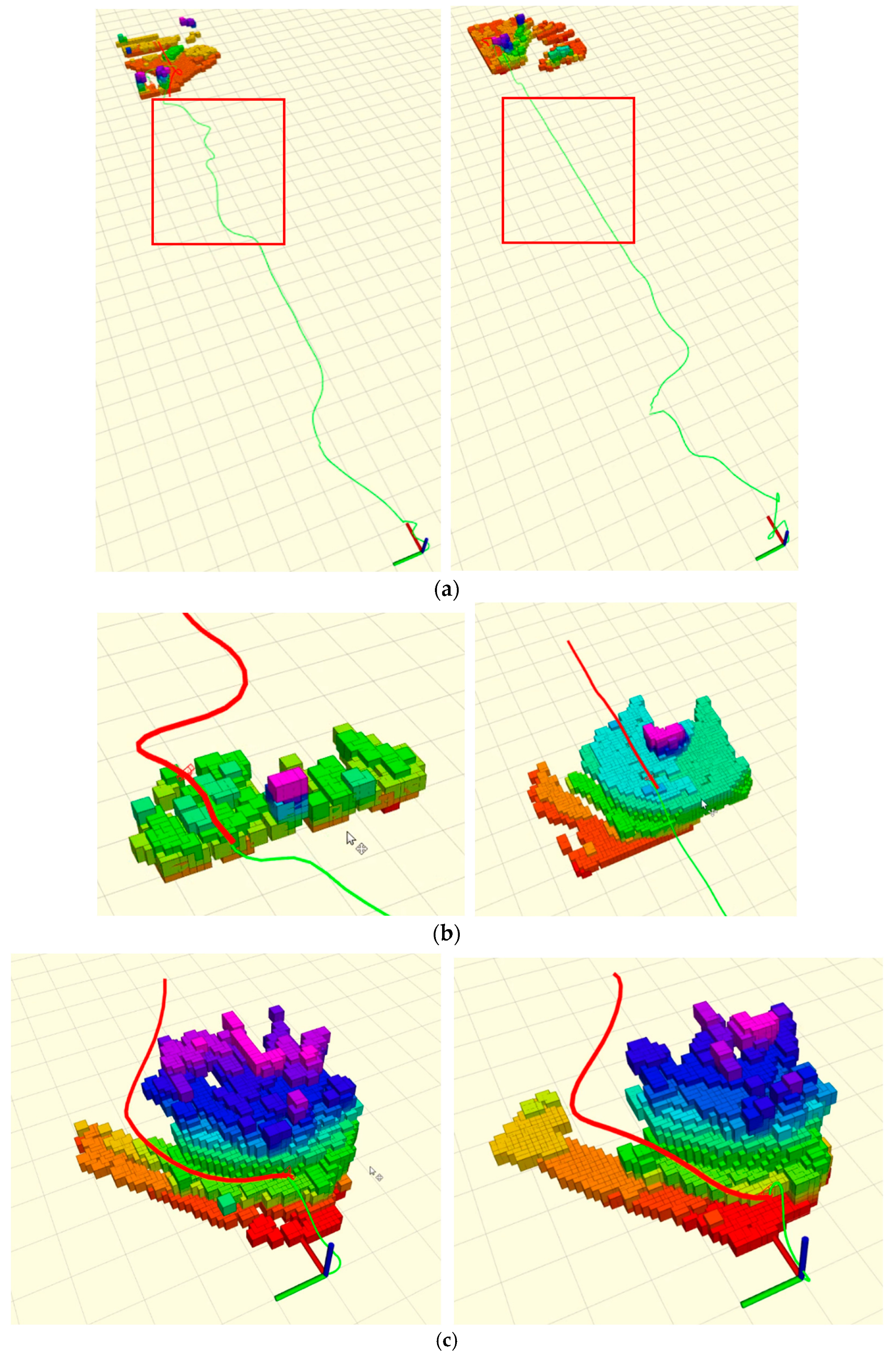
The comparison of Ego and Ours in real-world performance. The overall trajectories and local detail both show our method can generate more aggressive trajectories compared to Ego. (a) The real executed trajectory (left: Ego Right: Ours) shown in the green line. (b) The comparison of detail one (left: Ego Right: ours) in local planning. (c) The comparison of detail two (left: Ego Right: ours) in local planning.
Figure 19.
The comparison of Ego and Ours in real-world performance. The overall trajectories and local detail both show our method can generate more aggressive trajectories compared to Ego. (a) The real executed trajectory (left: Ego Right: Ours) shown in the green line. (b) The comparison of detail one (left: Ego Right: ours) in local planning. (c) The comparison of detail two (left: Ego Right: ours) in local planning.
Figure 20.
The extreme flight performance in the real world.
Figure 20.
The extreme flight performance in the real world.
Table 1.
Parameter setting in all simulation tests.
Table 1.
Parameter setting in all simulation tests.
| Parameter | | | | | |
| Ours | 1.0 | 0.8 | 0.1 | \ | 1.0 |
| Ego [3] | 1.0 | 0.8 | 0.1 | 0.2 | \ |
Table 2.
Performance in a low-density map.
Table 2.
Performance in a low-density map.
Low Density
Obstacle Number
30 | Dynamic Limits Setting | Planning Time (ms) | Flight Time (s) | Max Flight Velocity (m/s) | Mean Flight Velocity (m/s) |
| Ours | Ego | Ours | Ego | Ours | Ego | Ours | Ego |
= 4 m/s
= 6 m/s2 | 0.87 | 0.89 | 8.42 | 11.83 | 3.30 | 3.04 | 2.89 | 2.12 |
= 6 m/s
= 8 m/s2 | 0.91 | 0.90 | 5.71 | 7.35 | 5.23 | 4.74 | 4.28 | 3.54 |
= 8 m/s
= 10 m/s2 | 0.92 | 0.93 | 4.21 | 5.14 | 6.35 | 5.82 | 5.78 | 5.03 |
Table 3.
Performance in a middle-density map.
Table 3.
Performance in a middle-density map.
Low Density
Obstacle Number
50 | Dynamic Limits Setting | Planning Time (ms) | Flight Time (s) | Max Flight Velocity (m/s) | Mean Flight Velocity (m/s) |
| Ours | Ego | Ours | Ego | Ours | Ego | Ours | Ego |
= 4 m/s
= 6 m/s2 | 0.89 | 1.03 | 10.29 | 14.79 | 3.11 | 2.90 | 2.53 | 2.04 |
= 6 m/s
= 8 m/s2 | 1.02 | 1.22 | 7.63 | 9.95 | 4.98 | 4.31 | 3.79 | 3.26 |
= 8 m/s
= 10 m/s2 | 1.35 | 1.78 | 5.89 | 7.34 | 5.84 | 5.07 | 5.10 | 4.65 |
Table 4.
Performance in a high-density map.
Table 4.
Performance in a high-density map.
Low Density
Obstacle Number
70 | Dynamic Limits Setting | Planning Time (ms) | Flight Time (s) | Max Flight Velocity (m/s) | Mean Flight Velocity (m/s) |
| Ours | Ego | Ours | Ego | Ours | Ego | Ours | Ego |
= 4 m/s
= 6 m/s2 | 1.89 | 2.09 | 16.44 | 20.99 | 2.96 | 2.71 | 2.05 | 1.87 |
= 6 m/s
= 8 m/s2 | 2.57 | 2.78 | 10.91 | 15.60 | 4.33 | 4.12 | 3.22 | 2.90 |
= 8 m/s
= 10 m/s2 | 4.37 | \ | 8.78 | \ | 5.78 | \ | 4.19 | \ |
Table 5.
Hardware configuration information.
Table 5.
Hardware configuration information.
| Hardware | Name |
|---|
| Autopilot | CUAV V5+ |
| Depth Camera | RealSense D435i |
| Motor | TMotor F60 |
| ESC | Hobbywing Xrotor |
| Onboard Computer | Manifold 2C (i7–8th) |
Table 6.
Performance in real-world tests.
Table 6.
Performance in real-world tests.
| Dynamic Limits Setting | Planning Time (ms) | Flight Time (s) | Max Flight Velocity (m/s) | Mean Flight Velocity (m/s) |
|---|
| Ours | Ego | Ours | Ego | Ours | Ego | Ours | Ego |
|---|
= 2 m/s
= 3 m/s2 | 1.09 | 1.45 | 34.48 | 45.31 | 1.50 | 1.37 | 1.17 | 0.89 |
| Disclaimer/Publisher’s Note: The statements, opinions and data contained in all publications are solely those of the individual author(s) and contributor(s) and not of MDPI and/or the editor(s). MDPI and/or the editor(s) disclaim responsibility for any injury to people or property resulting from any ideas, methods, instructions or products referred to in the content. |
© 2023 by the authors. Licensee MDPI, Basel, Switzerland. This article is an open access article distributed under the terms and conditions of the Creative Commons Attribution (CC BY) license (https://creativecommons.org/licenses/by/4.0/).


