Article

Fractal Complexity of a New Biparametric Family of Fourth Optimal Order Based on the Ermakov–Kalitkin Scheme

by
Alicia Cordero
1,*,
Renso V. Rojas-Hiciano
2,
Juan R. Torregrosa
1 and
Maria P. Vassileva
3
1
Instituto de Matemática Multidisciplinar, Universitat Politècnica de València, Camino de Vera, s/n, 46022 Valencia, Spain
2
Escuela de Ciencias Naturales y Exactas, Pontificia Universidad Católica Madre y Maestra, Autopista Duarte Km 1.5, Santiago De Los Caballeros 51000, Dominican Republic
3
Instituto Tecnológico de Santo Domingo (INTEC), Av. Los Procéres, Santo Domingo 10602, Dominican Republic
*
Author to whom correspondence should be addressed.
Fractal Fract. 2023, 7(6), 459; https://doi.org/10.3390/fractalfract7060459
Submission received: 3 April 2023 / Revised: 24 May 2023 / Accepted: 31 May 2023 / Published: 3 June 2023
(This article belongs to the Special Issue Applications of Iterative Methods in Solving Nonlinear Equations)

Abstract

:
In this paper, we generalize the scheme proposed by Ermakov and Kalitkin and present a class of two-parameter fourth-order optimal methods, which we call Ermakov’s Hyperfamily. It is a substantial improvement of the classical Newton’s method because it optimizes one that extends the regions of convergence and is very stable. Another novelty is that it is a class containing as particular cases some classical methods, such as King’s family. From this class, we generate a new uniparametric family, which we call the KLAM, containing the classical Ostrowski and Chun, whose efficiency, stability, and optimality has been proven but also new methods that in many cases outperform these mentioned, as we prove. We demonstrate that it is of a fourth order of convergence, as well as being computationally efficienct. A dynamical study is performed allowing us to choose methods with good stability properties and to avoid chaotic behavior, implicit in the fractal structure defined by the Julia set in the related dynamic planes. Some numerical tests are presented to confirm the theoretical results and to compare the proposed methods with other known methods.

1. Introduction

Many problems in science, physics, economics, engineering, etc., need to find the roots of nonlinear equations of the form f ( x ) = 0 , where f : D C C is a real or complex function with some characteristics.
Frequently, there is not an algorithm to obtain the exact solutions of these equations, and we need to approximate them by means of iterative processes. One of the most widely used iterative methods is Newton’s method. It has a second order of convergence, and its iterative expression is (see, for example [1,2])
x k + 1 = x k f x k f x k , k = 0 , 1 ,
The convergence of Newton’s scheme depends on the initial estimate being “close enough” to the solution, but there is no guarantee that this assumption holds when modeling many real-world problems. In an attempt to address this problem, and to make the convergence domain wider, Ermakov and Kalitkin [3] proposed a damped version of Newton’s method for the equations with the general form
x k + 1 = x k λ k f ( x k ) f x k , k = 0 , 1 , ,
where λ k is a sequence of real numbers determined by a certain rule or algorithm. One of the forms that λ k can take is the Ermakov–Kalitkin coefficient
λ k = f x k 2 f x k 2 + f x k f ( x k ) f x k 2 , k = 0 , 1 ,
We can classify iterative methods [4] according to the data needed to determine the next value of the succession of approximations to the root. The method is memoryless if it depends on the value of the last iterate, not the previous ones:
x k + 1 = ϕ x k ; k = 0 , 1 , 2 ,
However, if the method contains memory, then it will also be a function of one or more of the iterates prior to the predecessor:
x k + 1 = ϕ x k , x k 1 , x k 2 , ; k = 0 , 1 , 2 ,
Iterative methods can also be classified [5,6] according to the number of steps in each iteration. Therefore, we consider either one-step or multi-step methods. A one-step method is in the form of the Equation (4), while a multi-step method is described by:
y k = ψ x k x k + 1 = ϕ x k , y k , k = 0 , 1 , 2 ,
For the study of the different iterative methods, we use the order of convergence as a measure of the speed at which the sequence { x k } k 0 generated by the method converges to the root. If lim k x k + 1 α / x k α p = C , where C and p are constants, then p represents the order of convergence.
If p = 1 and C 0 , 1 , we have linear convergence, but if p > 1 and C > 0 , the method has convergence of order p (quadratic, cubic, …)
An iterative method is said to be optimal, if it achieves convergence order 2 d 1 , using d functional evaluations at each iteration. According to the Kung–Traub conjecture [7], the order of convergence of any multi-step method without memory cannot exceed 2 d 1 , where d is the number of functional evaluations per iteration. Therefore, the order 2 d 1 is the optimal order.
When delving into the problem of nonlinear equations to find higher order iterative methods of convergence, methods arise that require, in general, increasing the number of functional evaluations, as well as the number of steps, thus obtaining multi-step methods whose form is the one expressed in [5]. In the following, we present five iterative multi-step procedures with a fourth order of convergence, four of them being optimal. We use them in the numerical tests of this research to compare with some members of the KLAM family.
We consider, for later comparison purposes, Newton’s scheme (an optimal second-order scheme), given by
x k + 1 = x k f x k f x k ; k = 0 , 1 , 2 ,
and Jarratt’s method, presented in [8], with convergence order four and iterative expression
y k = x k 2 3 f x k f x k , x k + 1 = x k 1 2 3 f y k + f x k 3 f y k f x k f x k f x k , k = 0 , 1 , 2 ,
The following schemes are two-step methods, the first one being Newton’s scheme: we start with Ostrowski’s method, [9], with order of convergence four and whose second step is:
x k + 1 = y k f x k f x k 2 f y k f y k f x k ; k = 0 , 1 , 2 ,
Moreover, King’s family of fourth-order methods [10] is given by
x k + 1 = x k f x k f x k f x k + ( β + 2 ) f y k f x k + β f y k f y k f x k ; k = 0 , 1 , 2 , ,
where β R . For β = 2 , Ostrowski’s scheme is obtained.
We also consider the fourth-order Chun method, [11],
x k + 1 = x k f x k f x k 1 + 2 f y k f x k + f y k 2 f x k 2 f y k f x k ; k = 0 , 1 , 2 ,
All these two-steps schemes are optimal according to the Kung and Traub conjecture. For the numerical tests, in the final section, we denote these methods as N2, J4, Os4, K4, and Ch4, respectively.
In order to improve Newton’s method, Budzko et al. in [12] proposed a triparametric family of iterative methods with two steps, using a damped Newton method in the first step (as a predictor). The second step (corrector) resembles the Ermakov–Kalitkin scheme (2), (3). The resulting iterative procedure involves the evaluation of three functions at each iteration,
y k = x k α f x k f x k , x k + 1 = x k f x k 2 b f x k 2 + c f y k 2 f x k f x k , k = 0 , 1 , ,
with α , b , and c , as complex parameters. Budzko et al. showed that if b = 1 α + 2 α 2 2 α 2 , c = 1 2 α 2 ( α 1 ) , a one-parameter family of two-step iterative methods for solving nonlinear equations with a third order of convergence was obtained for values of the parameter α other than 0 or 1. Through numerical tests, they showed that the numerical performance of this family was better, in several problems, than that presented by Newton’s method. We denote scheme (10) as the Budzco x-family or PM.
Cordero et al. in [13] carried out an in-depth study on the dynamics of the Budzco family and determined the convergence properties that allow this method to have a stable dynamical behavior for parameter values close to 0. They called the accelerating factor of the second step, f x k 2 b f x k 2 + c f y k 2 , the “Kalitkin-type factor”. This uniparametric family of methods managed to improve Newton’s, both in order of convergence [12] and in providing much larger basins of attraction. They showed that, for small values of the parameter, the basins of attraction that did not correspond to the roots of the polynomial were indeed small [13].
Our contribution is to present a new biparametric family of two-step iterative methods, also based on the Ermakov–Kalitkin scheme (Section 2) that improves the third order of Budzco’s family of methods and, hence, Newton’s, while keeping the same number of functional evaluations. We obtain a class of fourth-order optimal methods, with low computational cost. The dynamical analysis of the proposed family, with the stability of the fixed points, the behavior of the critical points, etc., are presented in Section 3. We devote Section 4 to the numerical tests and to comparing the proposed methods with other known ones. With some conclusions and the references used, we finish this manuscript.

2. Design and Analysis of the Methods

We want to increase the order of convergence of the iterative methods of the form given in (10) to the fourth order while maintaining the Kalitkin-type factor, and we achieve this, as we show, by finding a weight function introduced in the corrector step:
y k = x k α · g ( x k ) , x k + 1 = x k K μ k · H μ k · g ( x k ) , k = 0 , 1 ,
We include the weight function H μ k to increase the order of convergence of the method, without adding new functional evaluations.
Theorem 1.
Let ξ D be a simple zero of a function f of class C 4 , such that f : D C C in a convex set D, and let x 0 be an initial approximation close enough to ξ. The biparametric family defined by (11) has a fourth order of convergence whenever α = 1 , b 0 , for every weight function H : R R sufficiently differentiable, satisfying H ( 0 ) = H ( 0 ) = b , H ( 0 ) = 2 ( 2 b + c ) , and H ( 0 ) < . Moreover, the error equation is
e k + 1 = c 2 3 5 b + c H ( 0 ) b c 2 c 3 e k 4 + O e k 5 ,
where c k = ( 1 / k ! ) f ( k ) ( ξ ) f ( ξ ) for k = 2 , 3 , and e k = x k ξ .
Proof. 
By using Taylor’s series developments around ξ , we have the expressions for f ( x ) and f ( x ) , respectively,
f x k = f ( ξ ) e k + c 2 e k 2 + c 3 e k 3 + c 4 e k 4 + O e k 5 ,
f x k = f ( ξ ) 1 + 2 c 2 e k + 3 c 3 e k 2 + 4 c 4 e k 3 + O e k 4 .
From (12) and (13), we can obtain the error made in the first step of scheme (11),
y k ξ = ( 1 α ) e k + α c 2 e k 2 2 α c 2 2 c 3 e k 3 + α 4 c 2 3 7 c 2 c 3 + 3 c 4 e k 4 + O e k 5 .
Taylor’s series of f y k around ξ gives
f y k = f ( ξ ) ( 1 α ) e k + 1 α + α 2 c 2 e k 2 2 α 2 c 2 2 + 1 + α 3 α 2 + α 3 c 3 e k 3 + O e k 4 ,
and combining these equations, we obtain the expressions of μ k and K μ k , respectively:
μ k = f ( y k ) f ( x k ) = ( 1 α ) + α 2 c 2 e k α 2 ( 3 c 2 2 + ( 3 + α ) c 3 ) e k 2 + α 2 ( 8 c 2 3 + 2 ( 7 + 2 α ) c 2 c 3 + ( 6 + ( 4 + α ) α ) c 4 e k 3 + O e k 4 , K μ k = 1 b + c μ 2 = ρ 3 ( ρ 2 + ρ 2 γ α 2 c c 2 e k + α 2 c [ b 6 + 6 α + α 2 + 3 γ 2 γ 2 + 1 c c 2 2 2 γ ( α 3 ) ρ c 3 ] e k 2 ) + O e k 3 ,
where ρ = b + ( 1 + α ) 2 c , and γ = 1 + α .
Given that μ k tends to zero when x k tends to ξ , we develop in Taylor series H μ k around zero,
H μ k H ( 0 ) + H ( 0 ) μ k + H ( 0 ) 2 μ k 2 + H ( 0 ) 6 μ k 3 .
Therefore, using Equations (14) and (15), we have the error made in the second step.
e k + 1 = x k + 1 ξ = x k ξ K μ k · g ( x k ) · H μ k = ( 2 ρ ) 1 2 ρ + 2 H ( 0 ) + ( 2 H ( 0 ) + H ( 0 ) H ( 0 ) α ) γ e k + ( 2 ρ 2 ) 1 [ c γ 4 H ( 0 ) α 2 + 2 ( H ( 0 ) + H ( 0 ) ) γ + 2 H ( 0 ) α γ 2 + H ( 0 ) γ 3 + b 2 H ( 0 ) + H ( 0 ) 1 + α + 2 α 2 γ 2 H ( 0 ) α 2 + γ ] c 2 e k 2 + ρ 3 [ ρ α 2 ( H ( 0 ) + H ( 0 ) H ( 0 ) α ) ( b + c + c α ( 2 + ( 3 2 α ) α ) ) c 2 2 + 1 2 ρ 2 α 2 ( 6 H ( 0 ) + 6 H ( 0 ) H ( 0 ) α ( 6 + α ) ) c 2 2 + 2 ( 3 + α ) ( H ( 0 ) + H ( 0 ) H ( 0 ) α ) c 3 1 2 ( 2 H ( 0 ) + ( 2 H ( 0 ) + H ( 0 ) γ ) γ ) 2 b 2 + c 2 γ 2 ( 2 + α ( 2 + 3 α ) ( 2 + ( 2 + α ) α ) ) b c ( 4 + α ( 8 + α ( 12 + α ( 8 + α ) ) ) ) c 2 2 2 ρ b + c γ 1 + α 3 α 2 + α 3 c 3 ] e k 3 + O ( e k 4 ) .
Finally, if we require α = 1 , b 0 ,   H ( 0 ) = H ( 0 ) = b , H ( 0 ) = 2 ( 2 b + c ) , and H ( 0 ) < , then we cancel the coefficients of e k , e k 2 , and e k 3 in expression (16), and we obtain the error equation of the methods
e k + 1 = c 2 3 5 b + c H ( 0 ) b c 2 c 3 e k 4 + O e k 5 .
 ☐
Taking into account the convergence conditions of Theorem 1, by means of some algebraic manipulations and using as weight function the cubic Taylor polynomial, we obtain the iterative expression of the proposed method (11)
x k + 1 = y k 1 + 2 μ k + d μ k 2 1 + λ μ k 2 f ( y k ) f ( x k ) , k = 0 , 1 , ,
where y k is Newton’s scheme, and λ = c / b . This expression defines a family of two-parameter methods, λ and d, which we call Ermakov’s Hyperfamily (EH4).
Taking d = 0 in (18), we obtain a uniparametric family
y k = x k g ( x k ) , x k + 1 = y k 1 + 2 μ k 1 + λ μ k 2 f ( y k ) f ( x k ) , k = 0 , 1 , ,
which we call the KLAM family.
This family includes some known schemes as particular cases:
(i)
If λ = 4 , in the KLAM family, presented in (19), then we have Ostrowski’s classical method, described in iterative expression (7).
(ii)
If λ = β 2 and d = β ( β + 2 ) in the Ermakov Hyperfamily, presented in (18), then we have King’s Family, described in iterative expression (8).
(iii)
If λ = 0 and d = 1 , in the Ermakov Hyperfamily, presented in (18), then we have Chun’s fourth-order method, described in the iterative expression (9).

3. Dynamical Behavior of the KLAM Family

Complex dynamics has become, in recent years, a very useful tool to deepen the knowledge of rational functions obtained by applying iterative processes on low-degree polynomials p ( z ) . This knowledge gives us important information about the stability of the iterative method.
The tools of complex dynamics are applied to the rational function resulting from acting an iterative scheme on the quadratic polynomial p ( z ) = ( z a 1 ) ( z a 2 ) = 0 . When a parametric class of iterative algorithms is applied to p ( z ) , a parametric rational function is obtained. This analysis allows us to choose the members of the class with good stability properties and avoid the elements with chaotic behavior.
We recall some concepts of complex dynamics. Extended information can be found in [14].
Let R : C ^ C ^ be a rational function, where C ^ is the Riemann sphere. The orbit of a point z 0     C ^ is the set of successive images of z 0 by the rational function z 0 , R z 0 , R 2 z 0 , , R n z 0 , .
A point z 0 C ^ is a fixed point of R , if R ( z 0 ) = z 0 , and it is classified as attractor, a repulsor, and neutral or parabolic, if R z 0 < 1 ,   R z 0 > 1 , and | R z 0 | = 1 , respectively. When | R ( z 0 ) ) | = 0 , it is a superattractor. On the other hand, a point z 0 C ^ is a periodic point of period p > 1 , if R p z 0 = z 0 and R k z 0 z 0 , k < p . Finally, z 0 C ^ is a critical point of R, if R z 0 = 0 .
The basin of attraction A ( z ¯ ) of a fixed point (or periodic) attractor z ¯ C ^ is formed by the set of its pre-images of any order; that is, A ( z ¯ ) = z 0 C ^ : R n z 0 z ¯ , n + .
The Fatou set is formed by those points whose orbits tend to an attractor. The Julia set is the complementary set in the Riemann sphere of the Fatou set.
Theorem 2.
(Julia and Fatou [15,16]) Let R be a rational function. The basin of attraction of a periodic (or fixed) attractor point contains at least one critical point.
This last result has important consequences: by locating the critical points and calculating their orbits, we determine whether there can be other types of basins of attraction other than the roots of the polynomial. It is useful to analyze the behavior of a critical point used as the initial estimation of the iterative method; its orbit tends to a root of the polynomial or to another attractor element.
On the other hand, the scaling theorem allows us to extend the stability properties obtained for p ( z ) to any quadratic polynomial.

3.1. Rational Operator and Conjugacy Classes

We prove that the rational operator associated with the KLAM family, presented in (19), on p ( z ) = ( z a 1 ) ( z a 2 ) , satisfies the scaling theorem.
Theorem 3.
(Scaling theorem of the KLAM family) Let g ( z ) be an analytic function, and let A ( z ) = α z + κ , with α 0 , be an affine application. Let h ( z ) = γ ( g A ) ( z ) , with γ 0 . Let B g ( z ) be the fixed point operator of the KLAM method on p ( z ) . Then,
A B h ( z ) = B g ( z ) A ( z ) ;
that is, B g and B h are affine conjugate by A.
Proof. 
Let B g : C ^ C ^ be the fixed point operator of the KLAM family of methods, presented in (19), on a function g ( z ) ; that is
B g ( z ) = y ( z ) 1 + 2 ν ( z ) 1 + λ ν ( z ) 2 g y ( z ) g ( z ) ,
where
y ( z ) = z g ( z ) g ( z ) , and ν ( z ) = g ( y ) g ( z ) .
First, let us determine B g A ( z ) ,
B g A ( z ) = A ( y ( z ) ) 1 + 2 ν A ( z ) 1 + λ ν A ( z ) 2 g ( A ( y ( z ) ) ) g ( A ( z ) ) .
Now,
B h ( z ) = y ( z ) 1 + 2 ν ( A ( z ) ) 1 + λ ν ( A ( z ) ) 2 g A ( y ( z ) ) κ g ( A ( z ) ) .
As A ( m n ) = A ( m ) A ( n ) + κ , then
A B h ( z ) = A ( y ( z ) ) 1 + 2 ν ( A ( z ) ) 1 + λ ν ( A ( z ) ) 2 g A ( y ( z ) ) α g ( A ( z ) ) = A ( y ( z ) ) A 1 α 1 + 2 ν ( A ( z ) ) 1 + λ · ν ( A ( z ) ) 2 g A ( y ( z ) ) g ( A ( z ) ) + κ = A ( y ( z ) ) 1 + 2 ν ( A ( z ) ) 1 + λ ν ( A ( z ) ) 2 g A ( y ( z ) ) g ( A ( z ) ) .
So, it is concluded that the scaling theorem is satisfied by the KLAM family, presented in (19).  ☐
Now, we analyze the dynamical behavior of the fourth-order parametric family (19), studying the rational operator obtained to apply the family on the quadratic polynomial p ( z ) = ( z a 1 ) ( z a 2 ) . This operator depends on the roots of p ( z ) and parameter λ ,
B g ( z , a 1 , a 2 , λ ) = N D a 1 a 2 + 2 z ,
where
N = a 1 5 a 2 + 5 a 1 4 a 2 ( a 2 2 z ) + a 1 3 a 2 λ ( a 2 z ) 2 + 10 ( a 2 2 z ) 2 + a 1 2 5 a 2 4 2 a 2 3 ( λ + 20 ) z + 3 a 2 2 ( λ + 30 ) z 2 60 a 2 z 3 ( λ + 5 ) z 4 + a 1 a 2 5 10 a 2 4 z + a 2 3 ( λ + 40 ) z 2 60 a 2 2 z 3 + a 2 ( 20 3 λ ) z 4 + 2 ( λ + 7 ) z 5 z 4 a 2 2 ( λ + 5 ) 2 a 2 ( λ + 7 ) z + ( λ + 10 ) z 2 ,
and
D = a 1 2 a 2 2 λ 2 a 1 λ z 3 2 a 2 λ z 3 32 a 1 z 3 32 a 2 z 3 + a 1 2 λ z 2 + a 2 2 λ z 2 + 4 a 1 a 2 λ z 2 + 24 a 1 2 z 2 + 24 a 2 2 z 2 + 48 a 1 a 2 z 2 2 a 1 a 2 2 λ z 2 a 1 2 a 2 λ z 8 a 1 3 z 8 a 2 3 24 a 1 a 2 2 z 24 a 1 2 a 2 z + a 1 4 + a 2 4 + 4 a 1 a 2 3 + 6 a 1 2 a 2 2 + 4 a 1 3 a 2 + λ z 4 + 16 z 4 .
In order to eliminate the dependence of a 1 and a 2 , we apply the Möbius transformation
M ( z ) = z a 1 z a 2 ,
whose inverse is [ M ( z ) ] 1 = z a 2 a 1 z 1 . So,
E ( z , λ ) = ( M B g ( z , a 1 , a 2 , λ ) M 1 ) ( z ) = z 4 ( λ + z ( z + 4 ) + 5 ) z ( ( λ + 5 ) z + 4 ) + 1 .
The set of values of the parameter that reduces the expression of operator E ( z , λ ) is
10 , 5 , 4 , 2 , 1 , 0 .
We analyze the dynamics of this operator.

3.2. Stability Analysis of the Fixed Points

Both the number of fixed points and their stability depend on the parameter λ . We need to determine an expression for the differential operator, for analyzing the stability of the fixed points and to determine the critical points.
E ( z , λ ) = 2 z 3 λ 2 z 2 + 2 λ z ( z + 1 ) z ( z + 2 ) + 3 + 1 + 10 ( z + 1 ) 4 ( z ( ( λ + 5 ) z + 4 ) + 1 ) 2 .
It is not difficult to verify that both z = 0 and z = are superattracting fixed points, since they come from the zeros polynomial. However, the stability of the other fixed points depends on the value of λ .
Proposition 1.
The fixed points of rational operator E ( z , λ ) are the roots of equation E ( z , λ ) = z . Then, for each value of λ, it has the next fixed points:
(a)
z = 0 and z = are superattractor fixed points for any value of λ.
(b)
z = 1 is a fixed point, if and only if λ 10 .
(c)
The strange fixed points, ex1 ex2, ex3, and ex4 are 1 4 ϕ ± ϕ 2 ± 10 ϕ + 9 5 , where ϕ ( λ ) = 4 λ 7 .
  • In the following result, we analyze the stability of z = 1 .
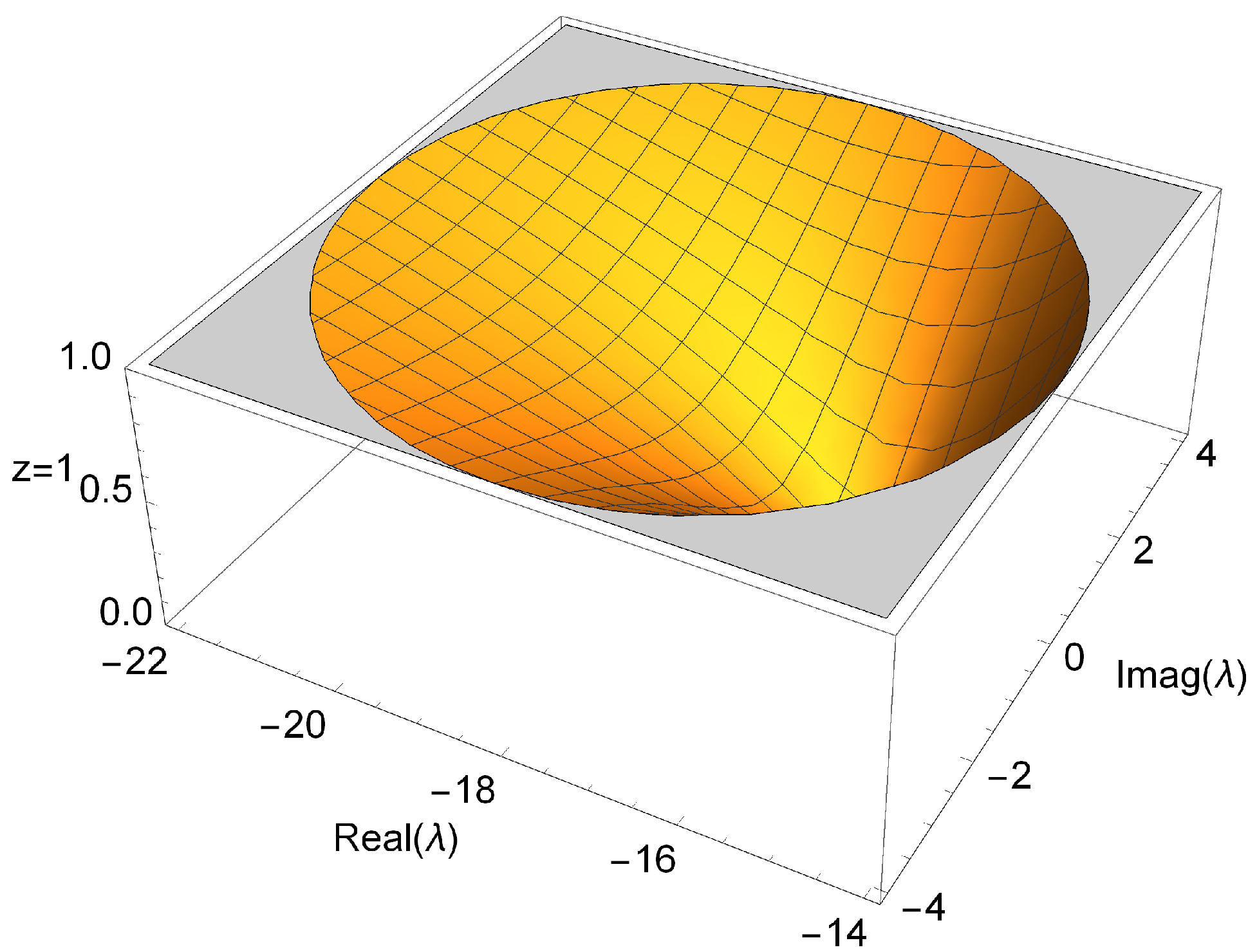
Theorem 4.
The character of the strange fixed point z = 1 , where λ 10 , is as follows:
(i)
z = 1 is an attractor, if and only if λ + 18 < 4 . It can be a superattractor for λ = 16 .
(ii)
z = 1 is a parabolic point in the circumference λ + 18 = 4 .
(iii)
z = 1 is a repulsor, if and only if λ + 18 > 4 ,   λ 10 .
Proof. 
First let us apply the operator E ( z , λ ) in (3.2) on z = 1 ,
E 1 , λ = 2 ( λ + 16 ) λ + 10 .
Let us analyze E ( 1 , λ ) < 1 , taking λ = w + i y , and after some algebraic manipulations, we have ( w + 18 ) 2 + y 2 < 16 , as shown in Figure 1. Then, the fixed point z = 1 is an attractor, if and only if
| λ + 18 | < 4 .
Analogously, the rest of the statements of the theorem are satisfied.  ☐
Now, we study the stability of the strange fixed points e x 1 , e x 2 , e x 3 , and e x 4 .
Theorem 5.
The character of the strange fixed points e x 1 and e x 2 is as follows:
  • If λ + 1 32 11 145 + 189 2 + 1 1024 11 145 + 133 2 < 1 16 11 145 + 133 λ + 7 4 , then e x 1 and e x 2 are attractors. They are superattractors for λ = 5 7 3 .
  • When λ + 1 32 11 145 + 189 2 + 1 1024 11 145 + 133 2 = 1 16 11 145 + 133 λ + 7 4 , e x 1 and e x 2 are parabolic points.
  • If λ + 1 32 11 145 + 189 2 + 1 1024 11 145 + 133 2 > 1 16 11 145 + 133 λ + 7 4 , then e x 1 and e x 2 are repulsors.
Proof. 
First, let us consider the stability function E ( z , λ ) on strange fixed points e x 1 and e x 2 :
E e x 1 , 2 , λ = ( M + ϕ + 5 ) 3 M ϕ 3 + 27 ϕ 2 265 ϕ + 45 + ϕ 4 + 32 ϕ 3 42 ϕ 2 1040 ϕ + 153 4 M ϕ 2 8 ϕ 33 + ϕ 3 + 17 ϕ 2 101 ϕ 93 2 ,
where M ( ϕ ) = ϕ 2 + 10 ϕ + 9 and ϕ ( λ ) = 4 λ 7 .
Let us make λ = w + i y , and after some algebraic manipulations, we have
E e x 1 , 2 , λ < 1 ,
if and only if
w + 1 32 11 145 + 189 2 + y 2 + 1 1024 11 145 + 133 2 2 < 1 256 11 145 + 133 2 w + 7 4 2 + y 2 ,
as shown in Figure 2. Therefore, e x 1 , 2 are attractors, if and only if
λ + 1 32 11 145 + 189 2 + 1 1024 11 145 + 133 2 < 1 16 11 145 + 133 λ + 7 4 .
Analogously, the rest of statements of the theorem are satisfied.  ☐
Theorem 6.
The character of the strange fixed points e x 3 and e x 4 is as follows:
(a)
If λ + 1 16 323 + 11 145 < 1 / 16 29 + 11 145 , then e x 3 and e x 4 are attractors. They are superattractors for λ = 5 3 + 7 .
(b)
In the circumference λ + 1 16 323 + 11 145 = 1 16 29 + 11 145 , or for λ = 7 4 , e x 3 and e x 4 are parabolic points.
(c)
If λ + 1 16 323 + 11 145 > 1 / 16 29 + 11 145 , λ 7 4 , then e x 3 and e x 4 are repulsors.
Proof. 
The stability function E ( z , λ ) on strange fixed points e x 3 and e x 4 is
E e x 3 , 4 , λ = ( P ϕ + 5 ) 3 ϕ 2 ( 14 M + 13 P + 219 ) + ϕ ( 111 M 154 P 355 ) ( M + 17 ) ϕ 3 + 9 ( 5 P + 17 ) 4 ϕ ( 13 M + 5 P + 102 ) + ( M + 9 ) ϕ 2 + 33 P + 93 2 ,
where P ( ϕ ) = ϕ 2 + 10 ϕ 9 , M ( ϕ ) = ϕ 2 + 10 ϕ + 9 , a n d ϕ ( λ ) = 4 λ 7 .
Let us make λ = w + i y , and after some algebraic manipulations, we have
E e x 3 , 4 , λ < 1 ,
if and only if
w + 1 16 323 + 11 145 2 + y 2 < 1 / 256 29 + 11 145 2 ,
as shown in Figure 2. Therefore, e x 3 , 4 are attractors, if and only if
λ + 1 16 323 + 11 145 < 1 / 16 29 + 11 145 .
In analogous way, the rest of the Theorem is proved.  ☐
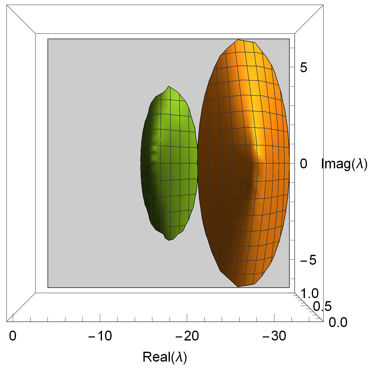
The strange fixed points for the values of the parameter that reduce the operator are the following:
(a)
λ = 10 :   e x 1 = 5.1792 ,   e x 2 = 0.19308 ,   e x 3 , 4 = 0.186141 ± 0.98252523 i ;
(b)
λ = 5 :   z = 1 ,   e x 1 = 4.05624 ,   e x 2 = 0.246534 ,   e x 3 , 4 = 0.348612 ± 0.937267 i ;
(c)
λ = 4 :   e x 3 , 4 = 0.5 ± 0.866025 i ;
(d)
λ = 2 :   z = 1 ,   e x 1 = 2.61803 ,   e x 2 = 0.381966 ,   e x 3 , 4 = 1 ;
(e)
λ = 1 :   z = 1 ,   e x 1 , 2 = 2.12196 ± 1.05376 i ,   e x 3 , 4 = 0.378036 ± 0.18773 i ;
(f)
λ = 0 :   z = 1 ,   e x 1 , 2 = 2.19428 ± 1.53703 i ,   e x 3 , 4 = 0.305725 ± 0.214151 i .

3.3. Analysis of Critical Points

From the definition of the critical point, given in Section 3.1, it is easy to prove that z = 0 and z = are critical points, for all values of the parameter. In addition, there are other critical points that we call “free”.
Theorem 7.
The rational operator has the following free critical points:
(i)
z = 1 , if λ 10 ,
(ii)
c r 1 , 2 = n s + λ m s ± C ( λ ) ,
(iii)
c r 3 , 4 = n s λ m s ± C ( λ ) ,
where
m = 2 λ 2 + 13 λ + 20 , n = 3 λ + 20 , n = λ + 5 , C ( λ ) = 2 λ 4 + 15 λ 3 + 80 λ 2 150 λ n s λ m s 3 .
The free critical points in the values reducing the operator are c r 1 , 2 = 2 ± 3 for λ = 10 ;   c r 1 , 2 = 1 4 ( 7 ± 33 ) for λ = 5 ; none for λ = 4 ;   c r 1 , 2 = 1 3 ( 4 7 ) for λ = 2 ;   c r 1 = 2 , c r 3 , 4 = 7 8 15 8 i for λ = 1 ; and z = 1 for λ = 0 .
Let us note that if λ = 4 , then the only fixed points are the roots of the polynomial, without free critical points. We can observe that it is among the best values that we can assign to the parameter, because it reduces the rational operator to x 4 . So, with this value our method has the most stable behavior.

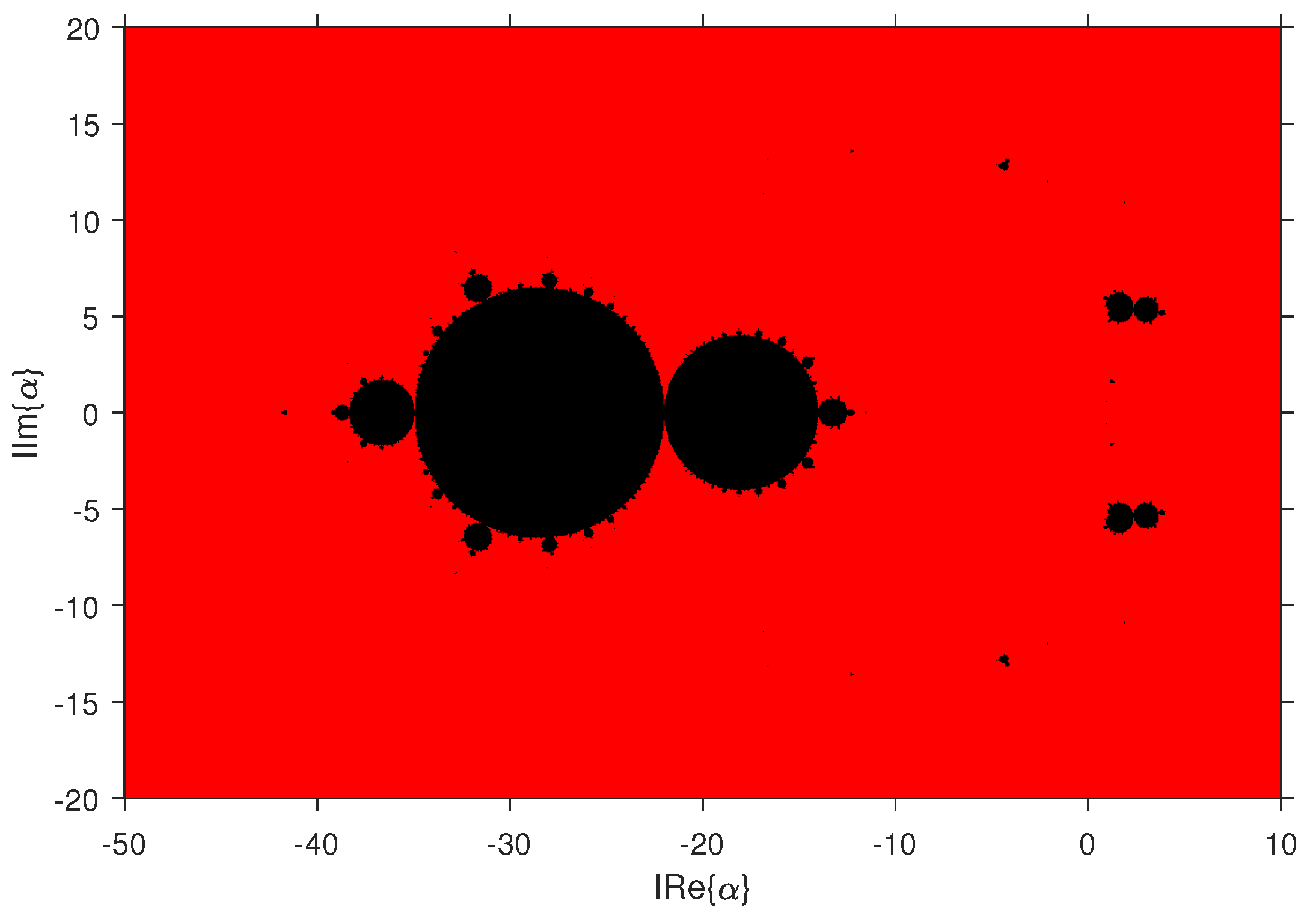
3.4. Parameter Planes of Critical Points

Chicharro et al. in [14] contributed to the generalized study of dynamic planes and parameter planes of families of iterative method. We conduct a similar study for the KLAM family (19).
There is one parameter plane for each independent free critical point. It is obtained by iterating the method taking as initial estimate each free critical point. We first define the mesh for complex values of the parameter and then consider each of its nodes as an element of the iterative method family. When iterating that method over the free critical point used as the initial estimate, we represent the parameter plane by assigning the color red or black, depending on whether that critical point converges to 0 or infinity, or not, respectively. The elements used are meshing in the desired domain, 500 × 500 points; the maximum number of iterations is 80, with tolerance 10 3 .
Let us now examine the two big regions that complete the study of the instability of the KLAM family of methods, based on the attractiveness of the fixed points, shown in Figure 3. The region where strangers 1 and 2 are attractors is very small and is not visualized in this graph, even if we consider the interval where it is contained.
Some regions where the extraneous fixed points are attractors, indicated in Figure 3, are the same in Figure 4 and Figure 5 that do not lead to the solution.

3.5. Dynamical Planes

To draw the dynamic planes, as with the Section 3.5 about parameter planes, we base our work on the contributions of Chicharro et al. in [14], applying the study to the KLAM family.
To generate the dynamical planes, we proceed in a similar way as for the parameter planes. In this case, parameter λ is constant, then the dynamical plane is related to a specific element of KLAM family. Each point of the plane is considered as an initial point in the iterative scheme, and different colors are used, depending on its convergence point.
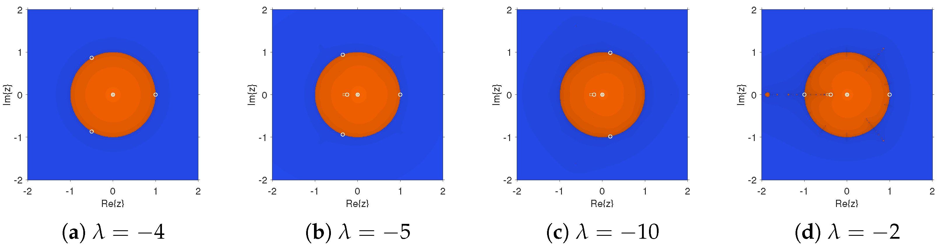
To obtain the dynamical planes, we used a mesh of 1000 × 1000 points of the complex plane, and a maximum of 200 iterations. We have chosen the parameter values shown in red in the parameter plane of the Figure 4 and Figure 5. We represent the superattractor fixed points with asterisk, the fixed points as circles, and the critical points as squares.
We took some values that simplified the parameter, as indicated in the Section 3.2, among others −4, −5, −10, and −2. These were the best choices for λ . We obtained the corresponding drawings in Figure 6.
According to Theorems 4–6 about the strange fixed points, we knew the values of the parameter for which they were attracting, repulsive, parabolic, or superattracting points. We presented the dynamical planes with some values, where all strange fixed points were repulsors, and we obtained the planes of the Figure 7. We noticed that only two basins appeared, corresponding to the superattracting z = 0 and z = . It can be seen that the larger the absolute value of λ , the more the method tended to a single shape.
The closer we moved to zero, the wider the basin of z = 0 , until it became compact at λ = 0 , where we had only two critical points, z = 0 and z = 1 , while the strange fixed points were z = 1 , e x 1 , 2 = 2.19428 ± 1.53703 i , and e x 3 , 4 = 0.30572525 ± 0.214151 i . We recall that with this value of λ , our scheme corresponded to Chun’s method.
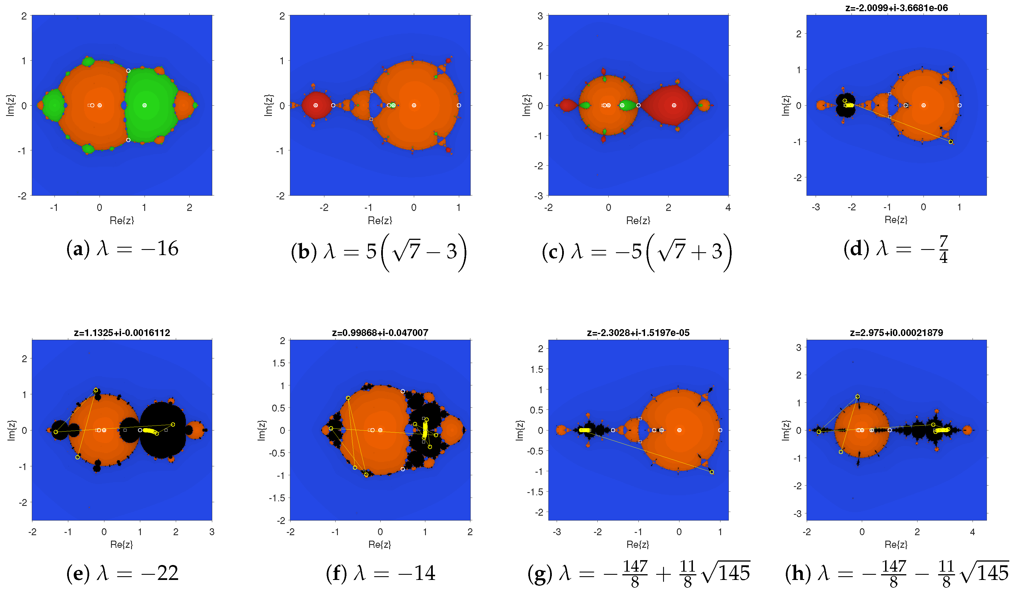
Figure 8 corresponds to values of the parameter where the strange fixed points were neutral or superattactors. In all these cases, there were three or four basins of attraction.

4. Computational Implementation

We compared three of the most stable elements of the KLAM family, specifically for λ 5 , 10 , 2 , and three of the more unstable methods of the family, as indicated in Theorems 4–6, where λ 22 , 16 , 5 ( 7 + 3 ) , which we call KLAM5, KLAM10, KLAM2, KLAM22, KLAM16, KLAM73, respectively; with the methods of Newton, Jarratt, (6), Ostrowski, (7), King ( β = 1 ), (8), and Chun, (9). These last four schemes are optimal methods of order four. We also compared our methods with the third-order scheme PM (10).
We used MATLAB R2020a for each of the tests, in a computer with the following specifications, Intel(R) Core(TM) i3-7100U CPU @2.40 GHz, 16 GB RAM.
The input parameters required for the programs of the iterative methods were the nonlinear function, the initial estimate previously deduced (approximated graphically), a tolerance of 10 15 , and a maximum number of iterations. We worked with 2000-digit variable precision arithmetic mantissa, and used as the stopping criterion x k + 1 x k + f x k + 1 . We provided as output the computational approximation of the order of convergence ACOC, the error estimates x k + 1 x k , the total error x k + 1 x k + f x k + 1 , the number of iterations “iter”, the approximate solution, and the time elapsed in seconds.
The nonlinear equations that we solved numerically were
  • f 1 ( x ) = c o s ( x ) x e x + x 2 = 0 , ξ 0.639154 .
  • f 2 ( x ) = 10 x e x 2 1 = 0 , ξ 1.6796306104284499 .
  • (Sphere floating in water) A sphere of density ρ e and radius r was partially submerged in water to a depth x, we calculated this depth:
    ρ a x 3 3 r ρ a x 2 + 4 ρ e r 3 = 0 , x 0 = 11 , ξ 11.8615 ,
    considering the density of water was ρ a = 1 g / cm 3 , the radius of the sphere was r = 10 cm and the wooden sphere of density was ρ e = 0.638 g / cm 3 .
  • (Compression of a real spring) An object of mass m was dropped from a height h onto a real spring, whose elastic force was F e = k 1 x + k 2 x 3 / 2 , where x was the compression of the spring; we calculated the maximum compression of the spring:
    m g h + m g x 1 2 k 1 x 2 2 5 k 2 x 5 / 2 = 0 , x 0 = 0.2 , ξ 0.1667 ,
    considering that the gravity was g = 9.81 m / s 2 ; the proportionality constants were k 1 = 40 , 000 g / s 2 ,   k 2 = 40 g / s 2 m 0.5 ; the mass of the object was m = 95 g ; and the height was h = 0.43 m .
By plotting the nonlinear functions whose zero we are looking for, we observed an initial estimate for the iterative process in each case.
Some numerical test results for various iterative schemes are presented in Table 1, Table 2, Table 3 and Table 4, where e k = | x k + 1 x k | and E k = e k + | F ( x k + 1 ) | .
We must take into account that the approximate computational order of convergence (ACOC), defined as
p A C O C = ln | x k + 1 x k | | x k x k 1 | / ln | x k x k 1 | | x k 1 x k 2 | .
We obtained the results detailed below.
  • Case 1: f 1 ( x ) = cos ( x ) x e x + x 2 , x 0 = 1.99 .
    KLAM5 was better, requiring only four iterations. All the unstable representatives diverged. The more stable ones behaved similarly and even better than the classical ones, as shown in Table 1.
  • Case 2: f 2 ( x ) = 10 x e x 2 1 ,   x 0 = 1.5 .
    This function had steep rises and falls. The only values that converged were the close ones to the solution, for all methods. The best performance was the KLAM5 with three iterations. All the other methods, even the unstable ones, converged and required, as the classical ones, four iterations, except N2 that needed six, as show in Table 2.
  • Case 3: f 3 ( x ) = x 3 30 x 2 + 2552 ,   x 0 = 13.8 .
    KLAM5 was better, requiring only three iterations. All others needed four, including the most unstable members of the KLAM family. KLAM2 was better than others, including classics. KLAM10 was behind Os4; but it was as J4, as shown in Table 3.
  • Case 4: f 4 ( x ) = 801 , 477 2000 + 18 , 639 20 x 20 , 000 x 2 16 x 2.5 ,   x 0 = 0.13 .
    For our last function, with real-world applications, KLAM5, KLAM2, and KLAM16 (unstable member) had the best performance with fewer iterations than all the others: four. The other two unstable representatives behaved as the classics in this problem, as shown in Table 4.

5. Conclusions

The biparametric Ermakov Hyperfamily, presented in this paper, improves the uniparametric Budzco third-order family, thus achieving a significant improvement over Newton’s method, since Budzco’s has wider regions of convergence and achieves a higher order than the latter. Our new family provides fourth-order optimal methods. This implies that many applied problems will be able to use our method, which is simple in its scheme but more powerful than Newton’s scheme.
This new family generalizes some important classical schemes, such as King’s family and Chun’s method, of proven application and reference for fourth-order methods. A new class, as a particular case of the Ermakov Hyperfamily, is the uniparametric KLAM family, also presented in this paper, whose dynamical behavior we have analyzed. It is a class of very stable iterative schemes for any value of the parameters, except in a few cases where a black region appears in the parameter plane, which is minuscule, compared to the stable region.
We note that Ostrowski’s method is a particular case, with λ = 4 , as it is Chun, with λ = 0 . The method performs very well with other values of the parameter λ 5 , 10 , 2 , outperforming in many cases this and the other classical methods in numerical tests. The best-performing representative in all the numerical tests was the KLAM5, corresponding to λ = 5 , which in the dynamical study for quadratic problems was higher than the fourth order.
The Ermakov Hyperfamily, with its subfamily KLAM, constitutes a significant contribution to the scientific community. We consider that we have a very stable family that can be extended to systems. If it behaves with similar stability in the vector case, we have a family that could be a reference for fourth-order methods in the multidimensional case.

Author Contributions

Conceptualization, A.C.; methodology, R.V.R.-H.; software, M.P.V.; validation, J.R.T.; formal analysis, A.C.; investigation, R.V.R.-H.; writing—original draft preparation, R.V.R.-H. and M.P.V.; writing—review and editing, A.C. and J.R.T.; supervision, J.R.T. All authors have read and agreed to the published version of the manuscript.

Funding

This research received no external funding.

Conflicts of Interest

The authors declare no conflict of interest.

References

  1. Ortega, J.M.; Rheinboldt, W.G. Iterative Solutions of Nonlinear Equations in Several Variables; Academic Press: New York, NY, USA, 1970. [Google Scholar]
  2. Traub, J.F. Iterative Methods for the Solution of Equation; Chelsea Publishing Company: New York, NY, USA, 1982. [Google Scholar]
  3. Ermakov, V.V.; Kalitkin, N.N. The optimal step and regularization for Newton’s method. USSR Comput. Math. Math. Phys. 1981, 21, 235–242. [Google Scholar] [CrossRef]
  4. Chicharro, F. Análisis dinámico y aplicaciones de métodos iterativos de resolución de ecuaciones no lineales. Ph.D. Thesis, Universitat Politècnica de València, Valencia, Spain, 2017. Available online: https://riunet.upv.es/bitstream/handle/10251/83582/Chicharro (accessed on 1 March 2023).
  5. Amorós, C. Estudio Sobre Convergencia y Dinámica de los Métodos de Newton, Stirling y Alto Orden. Ph.D. Thesis, Universidad Internacional de la Rioja, Madrid, Spain, 2020. Available online: https://reunir.unir.net/bitstream/handle/123456789/10259/TesisCristinaAmorosCanet.pdf?sequence=3 (accessed on 1 March 2023).
  6. Artidiello, S. Diseño, Implementación y Convergencia de Métodos Iterativos para Resolver Ecuaciones y Sistemas No Lineales Utilizando Funciones Peso. Ph.D. Thesis, Universitat Politècnica de València, Valencia, Spain, 2014. Available online: https://riunet.upv.es/bitstream/handle/10251/44230/ARTIDIELLO (accessed on 1 March 2023).
  7. Kung, H.T.; Traub, J.F. Optimal order of one-point and multi-point iteration. J. ACM 1974, 21, 643–651. [Google Scholar] [CrossRef]
  8. Jarratt, P. Some fourth order multipoint iterative methods for solving equations. Math. Comput. 1966, 20, 434–437. [Google Scholar] [CrossRef]
  9. Ostrowski, A.M. Solutions of Equations and Systems of Equations; Academic Press: Cambridge, MA, USA, 1966. [Google Scholar]
  10. King, R. A family of fourth order methods for nonlinear equations. SIAM J. Numer. Anal. 1973, 10, 876–879. [Google Scholar] [CrossRef]
  11. Chun, C.; Lee, M.Y.; Neta, B.; Dzunic, J. On optimal fourth-order iterative methods free from second derivative and their dynamics. Appl. Math. Comput. 2012, 218, 6427–6438. [Google Scholar] [CrossRef] [Green Version]
  12. Budzko, D.A.; Cordero, A.; Torregrosa, J.R. A new family of iterative methods widening areas of convergence. Appl. Math. Comput. 2015, 252, 405–417. [Google Scholar] [CrossRef]
  13. Cordero, A.; Torregrosa, J.R.; Vindel, P. Dynamical Analysis to Explain the Numerical Anomalies in the Family of Ermakov-Kalitkin Type Methods. Math. Model. Anal. 2019, 24, 335–350. [Google Scholar] [CrossRef] [Green Version]
  14. Chicharro, F.; Cordero, A.; Torregrosa, J.R. Drawing dynamical and parameters planes of iterative families and methods. Sci. World J. 2013, 2013, 780153. [Google Scholar] [CrossRef] [Green Version]
  15. Julia, G. Mémoire sur l’iteration des fonctions rationnelles. J. Math. Pures Appl. 1918, 8, 47–245. [Google Scholar]
  16. Fatou, P. Sur les équations fonctionelles. Bull. Soc. Math. Fr. 1919, 47, 161–271. [Google Scholar] [CrossRef] [Green Version]
Figure 1. Stability of the fixed point z = 1 .
Fractalfract 07 00459 g001
Figure 2. Stability of the fixed points e x 1 , 2 and e x 3 , 4 .
Fractalfract 07 00459 g002
Figure 3. Stability of the fixed points z = 1 , e x 3 and e x 4 .
Fractalfract 07 00459 g003
Figure 4. Parameter plane critical points c r 1 and c r 2 .
Fractalfract 07 00459 g004
Figure 5. Parameter plane critical points c r 3 and c r 4 .
Fractalfract 07 00459 g005
Figure 6. Parameter values with stable behavior.
Fractalfract 07 00459 g006
Figure 7. Good choices for parameter λ .
Fractalfract 07 00459 g007
Figure 8. Some poor parameter value choices.
Fractalfract 07 00459 g008
Table 1. f 1 ( x ) = cos ( x ) x e x + x 2 , x 0 = 1.99 .
MethodIter e k E k ACOC Time
N283.41444 × 10 21 3.41444 × 10 21 2.00060.039454
Os451.83671 × 10 40 2.75506 × 10 40 4.00030.046839
J451.83671 × 10 40 2.75506 × 10 40 3.99730.043834
K456.97665 × 10 21 6.97665 × 10 21 3.98390.052808
Ch451.79197 × 10 26 1.79197 × 10 26 3.99570.047364
PM52.48073 × 10 20 2.48073 × 10 20 3.03670.04878
KLAM543.78449 × 10 20 3.78449 × 10 20 3.95430.036386
KLAM1043.78449 × 10 20 3.78449 × 10 20 3.95430.036547
KLAM253.20552 × 10 33 3.20552 × 10 33 3.998360.049646
KLAM22-----
KLAM16-----
KLAM73-----
Table 2. f 2 ( x ) = 10 x e x 2 1 , x 0 = 1.5 .
MethodIter e k E k ACOC Time
N261.2344 × 10 27 1.23445 × 10 27 2.00000.036938
Os4403.67342 × 10 40 -0.043133
J4401.83671 × 10 40 -0.04651
K443.6734 × 10 40 5.51013 × 10 40 3.97450.046658
Ch443.6734 × 10 40 7.34684 × 10 40 3.81000.054437
PM41.7016 × 10 22 1.70159 × 10 22 2.99970.050942
KLAM534.911 × 10 16 4.91102 × 10 16 4.22730.05847
KLAM10403.67342 × 10 40 -0.062514
KLAM24 3.6734 × 10 40 1.65304 × 10 39 3.99830.047483
KLAM2245.5615 × 10 31 5.5615 × 10 31 4.00320.046064
KLAM1647.3990 × 10 36 7.3992 × 10 36 4.00160.048634
KLAM7342.88944 × 10 27 2.88944 × 10 27 4.0057-
Table 3. f 3 ( x ) = x 3 30 x 2 + 2552 , x 0 = 13.8 .
MethodIter e k E k ACOC Time
N251.0736 × 10 19 1.07356 × 10 19 2.00000.02148
Os442.9387 × 10 39 7.55255 × 10 37 4.12180.030254
J445.8775 × 10 39 7.58194 × 10 37 4.12180.038625
K4----
Ch442.9387 × 10 39 1.50757 × 10 36 4.20120.034046
PM44.6207 × 10 24 4.6207 × 10 24 3.08390.041648
KLAM534.0429 × 10 16 4.04291 × 10 16 4.07160.027226
KLAM1045.8775 × 10 39 1.51051 × 10 36 4.26890.037735
KLAM2401.5046 × 10 36 -0.035880
KLAM2242.9387 × 10 39 1.5076 × 10 36 4.57590.044499
KLAM1642.9387 × 10 39 1.5076 × 10 36 4.68770.040360
KLAM7342.9387 × 10 39 1.5076 × 10 36 4.58210.045410
Table 4. f 4 ( x ) = 801 , 477 2000 + 18 , 639 20 x 20 , 000 x 2 16 x 2.5 , x 0 = 0.13 .
MethodIter e k E k ACOC Time
N284.9684 × 10 22 4.96836 × 10 22 2.00000.052285
Os4508.74274 × 10 38 -0.056474
J4501.00744 × 10 37 -0.054038
K451.686 × 10 22 1.68602 × 10 22 3.97630.063776
Ch454.5335 × 10 27 4.53348 × 10 27 3.99060.066177
PM68.2652 × 10 40 4.99388 × 10 36 2.98530.046459
KLAM541.0841 × 10 16 1.08407 × 10 16 4.74610.056326
KLAM1052.0468 × 10 16 2.04679 × 10 16 4.93150.059874
KLAM249.18 × 10 41 8.75 × 10 38 4.25540.044578
KLAM22601.0074 × 10 37 -0.078946
KLAM1645.15 × 10 20 5.15278 × 10 20 6.58170.053013
KLAM7352.75 × 10 31 2.75289 × 10 31 4.00320.077310
Disclaimer/Publisher’s Note: The statements, opinions and data contained in all publications are solely those of the individual author(s) and contributor(s) and not of MDPI and/or the editor(s). MDPI and/or the editor(s) disclaim responsibility for any injury to people or property resulting from any ideas, methods, instructions or products referred to in the content.

