Article

Efficient Generators of the Generalized Fractional Gaussian Noise and Cauchy Processes

by
María Estrella Sousa-Vieira
* and
Manuel Fernández-Veiga
atlanTTic Research Center, Universidade de Vigo, 36310 Vigo, Spain
*
Author to whom correspondence should be addressed.
Fractal Fract. 2023, 7(6), 455; https://doi.org/10.3390/fractalfract7060455
Submission received: 17 April 2023 / Revised: 29 May 2023 / Accepted: 31 May 2023 / Published: 1 June 2023
(This article belongs to the Section Engineering)

Abstract

:
In the last years of the past century, complex correlation structures were empirically observed, both in aggregated and individual traffic traces, including long-range dependence, large-timescale self-similarity and multi-fractality. The use of stochastic processes consistent with these properties has opened new research fields in network performance analysis and in simulation studies, where the efficient synthetic generation of samples is one of the main topics. Nowadays, networks have to support data services for traffic sources that are poorly understood or still insufficiently observed, for which simple, reproducible, and good traffic models are yet to be identified, and it is reasonable to expect that previous generators could be useful. For this reason, as a continuation of our previous work, in this paper, we describe efficient and online generators of the correlation structures of the generalized fractional noise process (gfGn) and the generalized Cauchy (gC) process, proposed recently. Moreover, we explain how we can use the Whittle estimator in order to choose the parameters of each process that give rise to a better adjustment of the empirical traces.

1. Introduction

Fundamental network algorithms and key performance metrics in telecommunication networks and services, such as routing, delay, age of information, or buffer sizing, rely on accurate statistical traffic models capable of replicating the temporal and spatial correlation observable in many diverse packet streams [1,2]. Further, current networks have been architected to support data services for traffic sources that are poorly understood or still insufficiently observed, such as mMTC (massive machine-type communication) or URLLC (ultra reliable low-latency communications) in 5G/6G, for which simple, reproducible, and good traffic models are yet to be developed. Since, in the past, complex correlation structures were empirically observed both in aggregated and individual traffic traces, including long-range dependence (LRD) and large-timescale self-similarity (SS) [3,4,5,6,7,8,9,10,11,12,13,14], it is reasonable to expect that novel or modified flexible stochastic processes have to be analyzed for teletraffic and simulation analysis of such advanced communication services. A similar research effort was made when queuing models with fractal correlated input and the analysis of that on network performance [15,16,17,18,19,20,21,22,23,24,25,26] were thoroughly studied. These works demonstrated that second-order statistics, and their extreme manifestations as LRD and SS, lead to very slow decay of the queue backlogs, thus having a huge impact on loss and delay.
Apart from the specific application in communications networks, long-range dependent and self-similar processes appear in many other fields in science and engineering. In [27], the authors show examples in physics, chemistry and biology. They are also of interest in the analysis of several types of time series, such as meteorological and hydrological data, stock markets data, rare events in finance and insurance, or biometric signals [28] and recently in vehicular traffic data [29].
There are, in the literature, several classes of stochastic processes with LRD and/or SS properties which have been successfully used to model the complex time series of real traffic. These include fractional Gaussian noise [15] (fGn) and its recent generalization [30]; alpha-stable processes [31]; the Cauchy process and its generalization [32]; fractional ARIMA [33] (fARIMA); the sum of on–off sources with sojourn times following a heavy-tailed distribution [7]; the state process of a M/G/ queuing system [34]; and wavelet functions [35].
However, in addition to the analytical tractability and flexibility to give rise to different correlation functions, an important feature with these advanced models is computational efficiency in the numerical simulation of their sample paths, especially because when LRD or SS are present, very long synthetic sample paths are necessary for accurate simulations. In this regard, one major drawback of many direct generators is that these are efficient only because of the application of an off-line algorithm for the creation of the traces.
To overcome this drawback, in our previous work [36,37], we leveraged the singular properties of the occupancy process in the M/G/ queuing system to generate, at low computational cost, arbitrarily long sequences with arbitrary covariance function. The key idea is just to select the service time distribution of customers in the M/G/ according to a suitable discrete probability mass function, and take advantage of the memoryless property in the arrivals to implement a very fast discrete-event simulation of this elementary model. In this paper, we show how to select the service time distribution of the M/G/ system in order to obtain accurate and efficient generators of the generalized fGn process [38] and the generalized Cauchy process [39], two classes of processes that provide a powerful way to describe the multi-fractal phenomena of traffic [40] because they are indexed by two independent parameters.
As an application, we use these efficient generators to reproduce the covariance structure of a real traffic sequence. In order to estimate the parameters of the models, which are the input that the simulator needs, we apply the Whittle estimator [41,42,43], a sufficient and robust statistic that operates in the spectral domain.
The remainder of the paper is organized as follows. In Section 2, we review the main concepts related to short-range dependence (SRD), LRD and self-similarity. The generalized fGn process is presented in Section 3.1 and the generalized Cauchy process is Section 3.2. The main properties of the M/G/ process used in this work are described in Section 4. In Section 5.1 and Section 5.2, we describe the improved M/G/-based generator of the correlation structure of the gfGn and generalized Cauchy processes, respectively and in Section 5.3 we show some results related to the accuracy of the generators. In Section 6, we explain how we can use the Whittle estimator for fitting empirical traffic. Finally, in Section 7, we summarize the conclusions.

2. SRD, LRD and Self-Similarity

We briefly review in this section the definitions and main properties of self-similar stochastic processes and long-range statistical correlation [44].
A stationary stochastic process X = ( X n ) n 0 is said to have short-range dependence (SRD) whenever the sum of the covariance coefficients is convergent, i.e., k = 0 r k < , where r k : = E [ X k + i X i ] / E [ | X i | 2 ] . A class of processes having SRD is that wherein the covariance series decays exponentially:
lim k log r k k = c ( 0 , ) .
An equivalent condition to exponential decay is that the spectral density f X ( ω ) : = k = 0 r k e j ω k is bounded at the origin. If the sum of the covariance series is not convergent, the process X is termed long-range dependent (LRD). An example of LRD processes is the broad class of processes having sub-exponential (e.g., hyperbolic) decay:
lim k log r k log k = α ( 0 , 1 )
so r k = o ( k α ) . In this case, the spectral density of X has a singularity at the origin.
Self-similarity is defined based on the properties of the covariance function of the aggregated process X ( m ) = ( X j ( m ) ) j 1 built from X when X has finite variance. This is the average of X over non-overlapping blocks of length m
X j ( m ) : = 1 m k = ( j 1 ) m + 1 j m X k .
Then, X is called exactly second-order self-similar with similarity parameter H [45] if m 1 H X ( m ) has the same covariance function as X for all m. This means that the aggregated process shows the same statistical correlation over time as the original process X . The covariance function of a self-similar process is
r k H = 1 2 ( k + 1 ) 2 H 2 k 2 H + ( k 1 ) 2 H k 1 .
Thus,
lim k r k H k 2 H 2 = ( 2 H 1 ) H ,
that is, r k H decays hyperbolically (as in (2)) with α = 2 H 2 . Clearly, X possesses LRD when H ( 0.5 , 1 ) . The covariance function (4) implies a spectral density given by
f H ( ω ) = c | e j ω 1 | 2 i = | 2 π i + ω | 2 H 1 , ω [ π , π ] ,
where c is a normalization constant such that π π f H ( ω ) d ω = Var [ X ] .
When (4) holds asymptotically, and, in addition, the convergence condition lim m = r k ( m ) = r k H for all k 1 is satisfied, then the process is called asymptotically second-order self-similar. Clearly, for asymptotic self-similarity, the spectral density converges to that of a self-similar process lim m f X ( m ) ( ω ) = f H ( ω ) for any ω [ π , π ] . It is not hard to see that a stationary process with a covariance function with hyperbolic decay, such as (2), is asymptotically second-order self-similar.
Stationary Gaussian processes are not always exactly or asymptotically self-similar, but it is known that they satisfy a property of local self-similarity as defined in [46]. The covariance function function r k is
r k = 1 c k α 1 + O ( k α )
for k 0 , where 0 < α < 2 is the order of the process. The so-called fractal dimension is δ = 2 α 2 . Therefore, the behavior of the covariance function near the origin determines the local irregularity of the process, and larger values of δ imply more irregularity (or burstiness) at small timescales.

3. Generalized Self-Similar Gaussian Processes

3.1. Generalized Fractional Gaussian Noise

Let B H ( t ) denote a fractional Brownian motion process [47]. Then, its sequence of discrete increments X n : = B H ( n ) B H ( n 1 ) , n = 1 , 2 , is an exactly self-similar stationary Gaussian process, known as fractional Gaussian noise (fGn). Since self-similarity is exact, its covariance function and spectral density are given by (4) and (6), respectively. Despite its fixed covariance structure, the fGn process is known to be a good approximation of the aggregation of more complex LRD Gaussian and non-Gaussian processes [48,49].
In [38], the generalized fractional Gaussian noise (gfGn) is introduced, with parameters 0 < H < 1 and 0 < a 1 . This is a Gaussian process with covariance function
r k H , a = 1 2 | k a | + 1 2 H + | | k a | 1 | 2 H 2 | k a | 2 H k 1 ,
that can be approximated by r k H , a H ( 2 H 1 ) | k a | 2 H 2 , so the LRD condition is clearly satisfied if 0.5 < H < 1 . The spectral density function of gfGn is [50]
f H , a ( ω ) = sin ( H a π ) Γ ( 2 H a + 1 ) | ω | 2 H a 1 + 1 2 k = 0 ( 1 ) k 1 Γ ( 2 H + k ) Γ ( a ( 2 H k ) + 1 ) Γ ( 2 H ) Γ ( 1 + k ) sin a ( 2 H k ) π 2 | ω | a ( 2 H k ) 1 ,
which can be approximated as
f H , a ( ω ) H ( 2 H 1 ) sin ( a π ( H 1 ) ) Γ ( 2 a H 2 a + 1 ) | ω | 2 a ( H 1 ) 1 .
The latter implies that f H , a ( 0 ) , which is actually the LRD condition reflected in the spectral domain. Figure 1 shows the analytical covariance function for different values of the parameters. It is increasing in H (for fixed a), and decreasing in a (for fixed H).

3.2. Generalized Cauchy Process

The generalized Cauchy process X C = ( X n ) n 1 with parameters 0 < α 2 and β > 0 is a stationary Gaussian process with an autocorrelation function given by [39,51]
ρ k β , α = ( 1 + k α ) β α , k 1 .
The covariance function ρ k β , α is positive-definite for the above ranges of α and β , and it is completely monotone for 0 < α 1 and β > 0 . When α = β = 2 , one obtains the usual Cauchy process. Since lim k k β ρ k β , α = 1 , this process is LRD for 0 < β < 1 . Notice that H = 1 β 2 .
Its spectral density function is [52]
f β , α ( ω ) = k = 0 ( 1 ) k Γ ( β α + k ) π Γ ( β α ) Γ ( 1 + k ) I 1 ( ω ) sin ( ω ) ω + k = 0 ( 1 ) k Γ ( β α + k ) π Γ ( β α ) Γ ( 1 + k ) π I 2 ( ω ) I 2 ( ω ) sin ( ω ) ω .
Here,
I 1 ( ω ) = 2 sin α k π 2 Γ ( α k + 1 ) | ω | α k 1 ,
and
I 2 ( ω ) = 2 sin ( β + α k ) π 2 Γ 1 ( β + α k ) | ω | ( β + α k ) 1 .
Letting ω 0 , the behavior of the spectral density function (12) is well approximated by
1 cos β π 2 Γ ( β ) | ω | β 1 ,
so f β , α ( 0 ) . This is, again, the LRD condition reflected in the spectral domain. Figure 2 plots the analytical autocorrelation function for different values of α , β .

4. The M/G/ Process

The M/G/ process [53] is the stationary limit of the state of a M/G/ queuing system, a queuing model with Poisson arrivals, general independent and identically distributed service times distributed as the random variable S, and an unlimited number of servers. Instead of the usual view as a continuous-time process, it is more convenient in our case to discretize time and look at the number of servers occupied at time t Z + [36], which can be written as
X t = i = 1 A t , i ,
where A t , i denotes the number of arrivals at time t i that are still in service at time t. Note that A t , i counts how many active customers have age i. For any fixed t, ( A t , i ) i 1 , form a collection of independent and identically distributed Poisson random variables with parameter λ P ( S i ) , where λ is the average arrival rate. It is easy to calculate the expectation and variance if X t :
E ( X t ) = Var ( X t ) = λ i = 1 P ( S i ) = λ E ( S ) .
The discrete-time process ( X t ) t 0 is stationary and time reversible. Its covariance function is
γ k = i = k + 1 P ( S i ) E ( S ) , k = 0 , 1 ,
Additionally, by (18), knowledge of the covariance function uniquely gives the probability mass function of the service time S because
P ( S = k ) = ( γ k 1 2 γ k + γ k + 1 ) E ( S ) , k = 1 , 2 ,
By (19), the autocovariance is non-negative and convex. Conversely, if a real-valued sequence γ k is non-negative, decreasing, and integer-convex, then it is a valid autocovariance sequence for some M/G/ discrete-time process [34]. If the latter assumptions hold, then lim k γ k = 0 , and the probability mass function of S is exactly (19).
( X t ) t 0 is stationary and ergodic under two assumptions:
A1
At start t = 0 , the number A 0 , 0 of customers in the system follows a Poisson probability mass function with expected value λ E ( S ) .
A2
These A 0 , 0 customers have a service time S ^ given by a distribution
P ( S ^ = k ) = P ( S k ) E ( S ) ,
which is that of the residual (or excess) life of S.
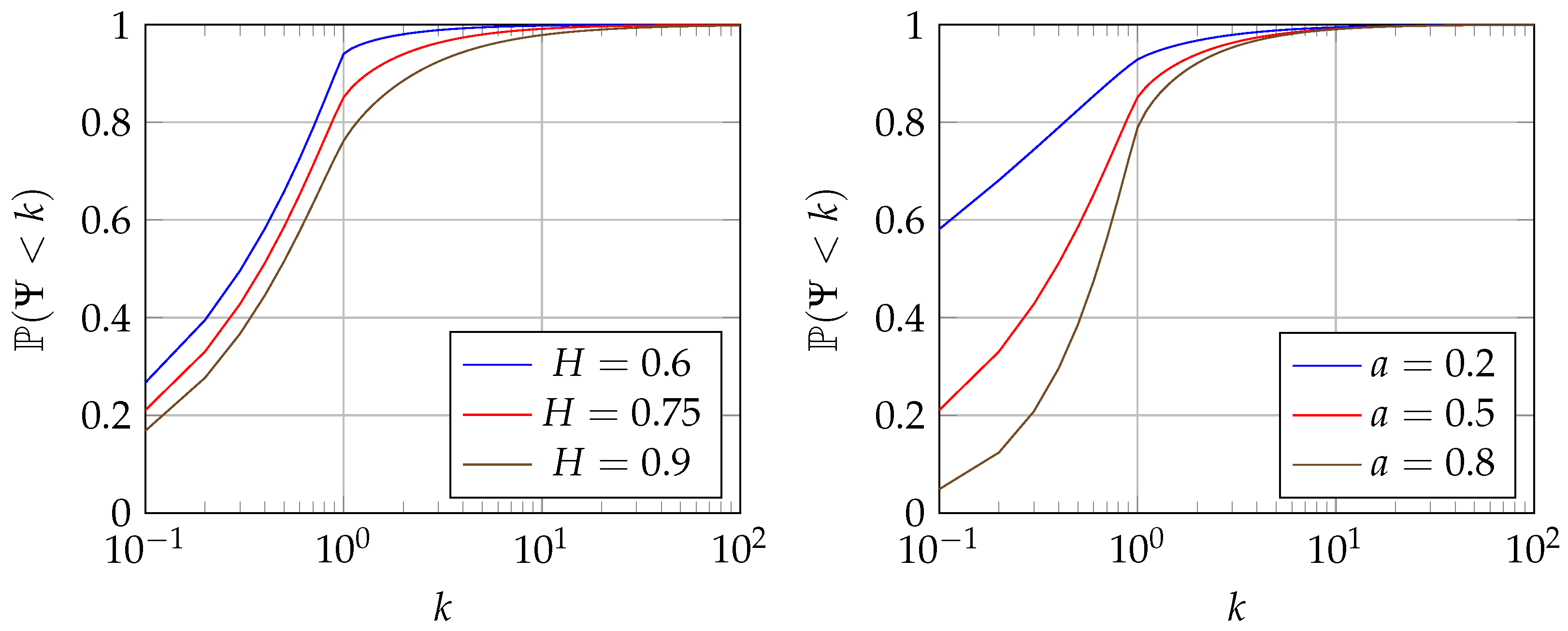
We have, as a consequence of this initial state, that (i) X t is Poisson for all t, with an expectation equal to λ E ( S ) , and (ii) the covariance function is γ k = γ 0 P ( S ^ > k ) k 0 . Therefore, ( X t ) t 0 is LRD when S has infinite variance, for instance, whenever S has some specific discrete heavy-tailed distributions. The latter means that P ( S > k ) c k q as k .

5. M/G/-Based Generation of Covariance Functions

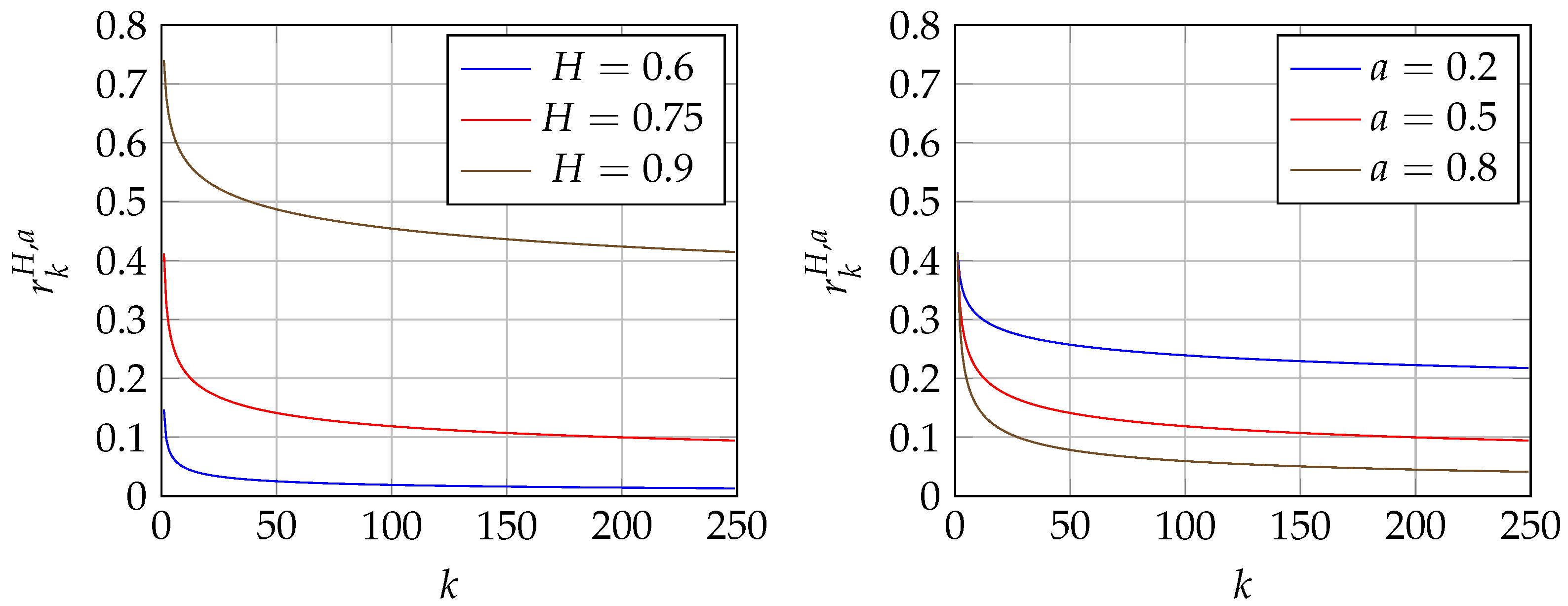
5.1. The gfGn Process

Denote by Ψ the service time in a M/G/ system, whose occupancy process has the covariance structure of the gfGn process. We know that at any time t, the distribution of Ψ is Poisson and converges weakly to a normal distribution when the mean goes to . Specifically, combining (18) and (19), the distribution function is
P ( Ψ < k ) = 1 0.5 ( | k a | + 1 ) 2 H + | k a | 1 2 H 2 | k a | 2 H 2 2 2 H 1 + 0.5 ( | ( k + 1 ) a | + 1 ) 2 H + | | ( k + 1 ) a | 1 | 2 H 2 | ( k + 1 ) a | 2 H 2 2 2 H 1
and the expected value is
E ( Ψ ) = 1 2 2 2 H 1 .
The distribution function of the residual life is needed in order to initialize the process in a steady state. It can be obtained from (18) and (20)
P ( Ψ ^ < k ) = 1 0.5 ( | k a | + 1 ) 2 H + | k a | 1 2 H 2 | k a | 2 H .
In Figure 3, we plot the analytical distribution function of the random variable Ψ for different values of the parameters.

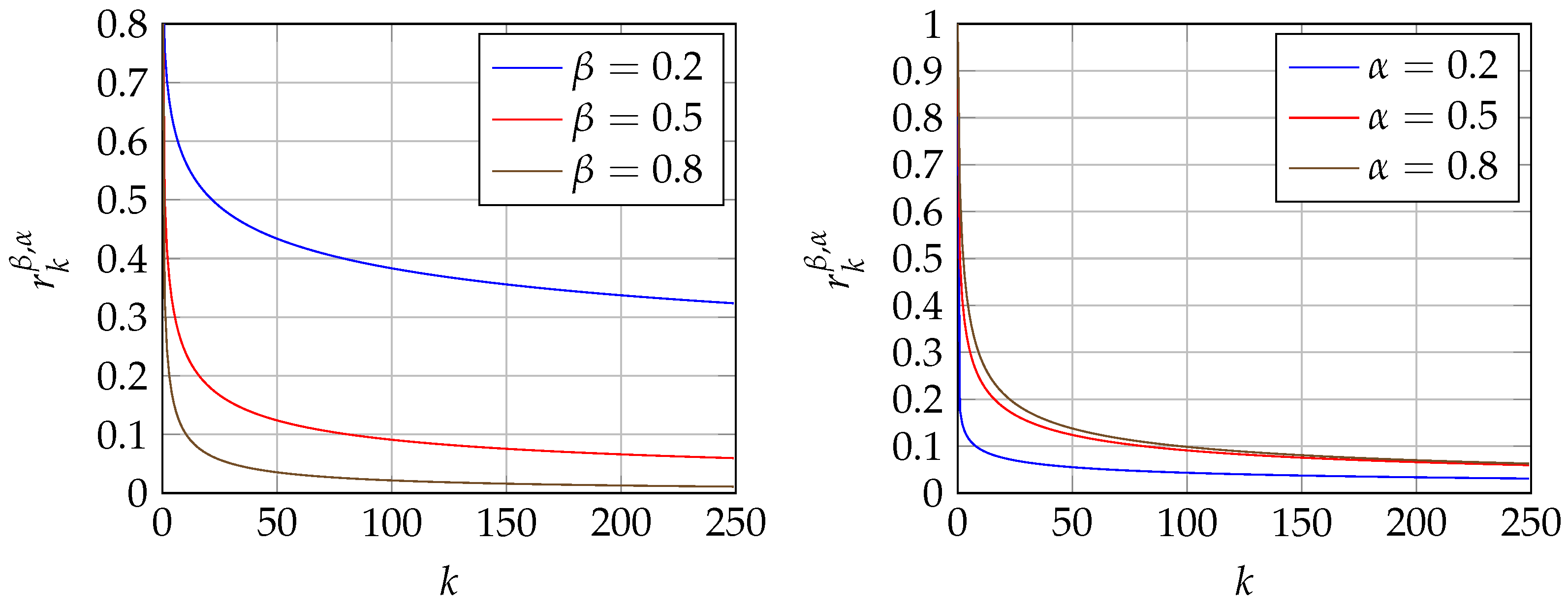
5.2. The Generalized Cauchy Process
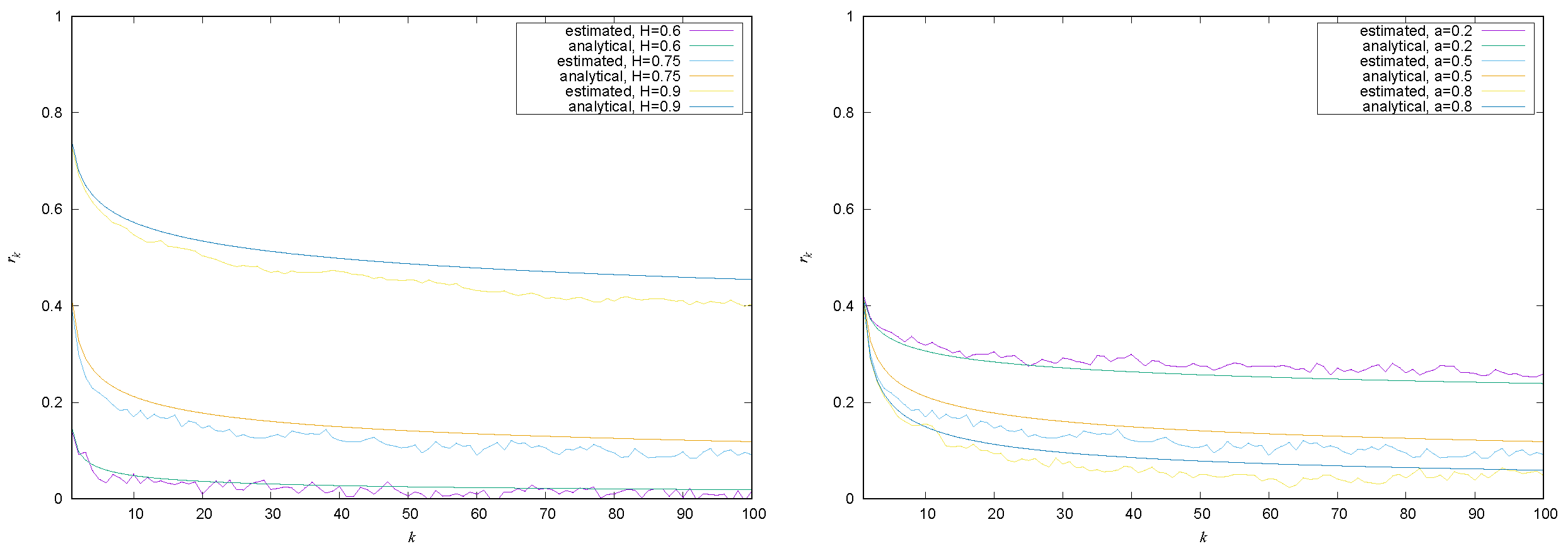
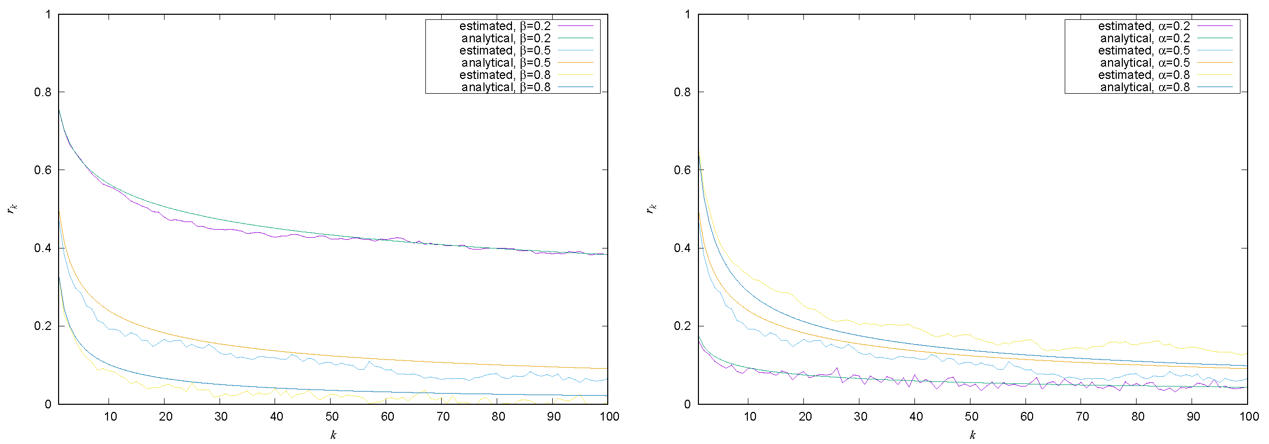
Now, let Ξ be the service time in a M/G/ system with an occupancy process that possesses the covariance structure of the generalized Cauchy process. By (11) and (18), the cumulative distribution function of Ξ is given by
P ( Ξ < k ) = 1 ( 1 + k α ) β α ( 1 + ( k + 1 ) α ) β α 1 2 β α ,
and the expected value E ( Ξ ) is
E ( Ξ ) = 1 1 2 β α .
For the excess life, the distribution function is, in this case,
P ( Ξ ^ < k ) = 1 ( 1 + k α ) β α .
In Figure 4, we can see the analytical distribution function of the random variable Ξ for different values of the parameters.

5.3. Accuracy

Since both distributions (21) and (24) have sub-exponential decay, the method that we developed in [37] can be used. That technique relies on the elementary properties of Poisson processes (decomposition and lack of memory) so that the M/G/ state process can be simulated very fast and sequentially. Moreover, the technique is flexible, i.e., valid for any distribution of the service time with sub-exponential decay. Specifically, [37] presents a fast tabular inversion method for generating the samples of S i , the service times in the queuing systems. When this tabular inversion is combined with the geometric (memoryless) interarrival times, the system state (16) can be calculated with only a few elementary operations, without any function evaluations.
The tabular method used for inversion in [37] produces some loss of numerical precision in the tail of some heavy-tailed distributions. Ref. [54] describes an improvement of the original method to solve this issue and also an extension to handle random variables with long tails in both sides. In this way, the Poisson arrival process in the case of high mean values can be also be generated using a better tabular method.
Figure 5 and Figure 6 show the estimated autocorrelation function of several traces generated with the proposed method for different values of the parameters of the generalized fGn process and the generalized Cauchy process, respectively. We can see that the estimations match well the analytical functions.

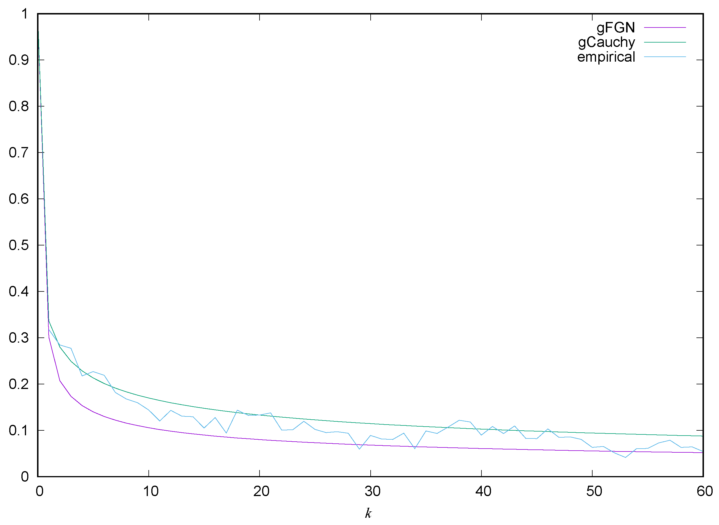
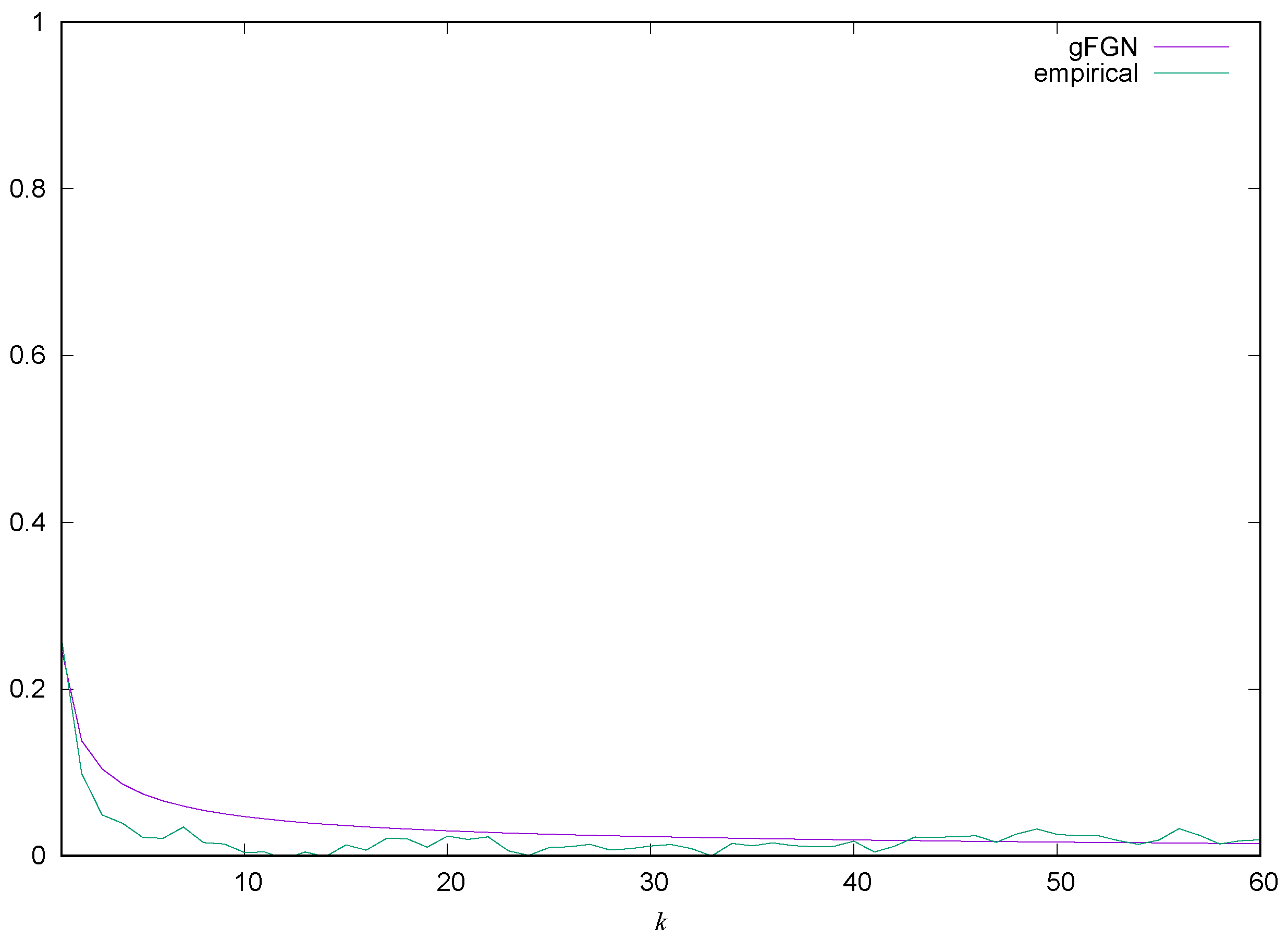
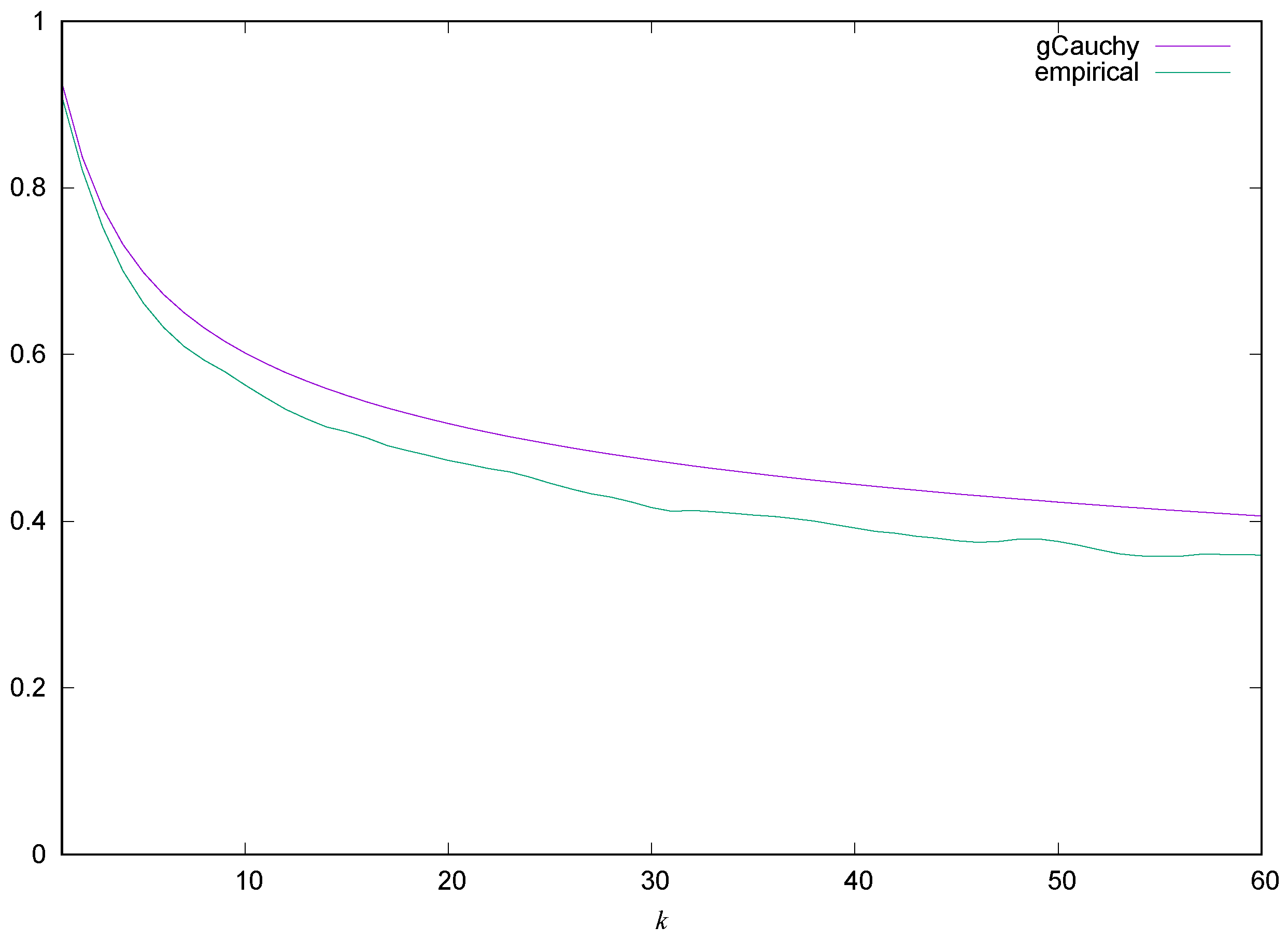
6. Modeling Eempirical Traces

In this section, we explain a method to estimate the parameters of the previous processes, gFGN and gCauchy, that give rise to a better adjustment of the spectral density and therefore of the correlation structure of the empirical traffic. The method is based on the Whittle estimator [41,42] that we describe briefly in the next section.

6.1. Whittle’s Estimator

Let f θ ( λ ) be the spectral density function of a zero-mean stationary Gaussian stochastic process X = ( X n ) n 0 , where θ = θ 1 , , θ M is a vector of unknown parameters to be estimated from observations. Let
I X ( ω ) = 1 2 π N i = 0 N 1 X i e j ω i 2
be the empirical periodogram obtained using N samples of the process X , where · is the Euclidean norm. The Whittle estimator [41] is the vector θ ^ = θ 1 ^ , , θ M ^ that minimizes the statistic
θ ^ = arg min θ Q X ( θ ) = 1 2 π π π I X ( ω ) f θ ( ω ) ω + π π log f θ ( ω ) ω .
Whittle’s estimator (28) approximates the Gaussian log-likelihood by means of the periodogram, using the latter in place of the unknown spectral density. Another information-theoretic interpretation is that Q X ( θ ) is the divergence between the periodogram I X ( · ) and f θ ( · ) .
Whittle’s estimator converges in probability to the true value θ o . It holds that
lim N P θ ^ θ o < ϵ = 1
for any ϵ > 0 , so θ ^ is a weakly consistent estimator. A second property is that it is also asymptotically normal; N ( θ ^ θ o ) ζ converges in distribution to ζ for large N, where ζ is a zero-mean Gaussian vector with a matrix of covariances known. This asymptotic normality allows the computation of confidence intervals for the estimated values.
It is also possible to choose a special scale parameter
θ 1 = exp 1 2 π π π log f θ ( ω ) ω = σ ϵ 2 2 π
such that f θ ( ω ) = θ 1 f ν * ( ω ) and the second term in (28) is zero. In this case, σ ϵ 2 is the optimal one-step-ahead prediction error that is equal to the variance of the innovations in the AR() representation of the process, and Whittle’s function (28) simplifies to
Q X ( ν ) = π π I X ( ω ) f ν ( ω ) ω .
The approximate Whittle estimator is usually evaluated numerically via the integral quadrature, replacing the integral by a sum over a discrete set of Fourier frequencies ω k = k π n ; k = n , , 1 , 0 , 1 , , n . In addition, it can be shown that the mean squared error is σ ϵ 2 ^ = Q X ( ν ) , where ν is the minimizer of (31).
In the past, we proposed to use σ ϵ 2 ^ as a measure of the suitability of a model because smaller values mean more accurate adjustment to the actual covariance function of the sample and suggest a close match between the sample and the model. Moreover, we used this value to compare the accuracy or convenience of different models. Specifically, in [37], we presented a method for model selection based on fitting the spectral density and, therefore, the empirical correlation function, and in [55], we tested the method numerically for several classes of stochastic processes, namely Gaussian and non-Gaussian processes with LRD, non-stationary processes and non-linear heteroscedastic models.

6.2. Examples

In this section, we show several examples that illustrate the suitability of these processes to model different kinds of network traffic. In these examples, we consider empirical traces that usually are used as examples of correlated traffic.
The capture of the trace of the first example was performed at the beginning of the last decade of the previous century [56]. This trace contains 2000 samples of Ethernet data lengths. The sample mean and variance are, approximately, μ ^ = 380 and σ 2 ^ = 180,100. In this case, both gFGN and gCauchy processes are able to approximate this trace quite well. The estimations of the parameters of each process, obtained via the Whittle estimator, are as follows:
  • gFGN process: H ^ = 0.696 and a ^ = 0.649 .
  • gGauchy process: β ^ = 0.503 and α ^ = 0.321 .
Figure 7 shows the correlation structure of this empirical trace versus the analytical autocorrelation of each process, with the estimated parameters.
The capture of the trace of the second example was performed in the middle of the first decade of this century [57]. This trace contains 2000 samples of TCP data lengths. The sample mean and variance are, approximately, μ ^ = 136 and σ 2 ^ = 46,750. In this case, only the gFGN process approximates this trace well. The estimators of its parameters, obtained via the Whittle estimator, are H ^ = 0.661 and a ^ = 0.961 . Figure 8 shows the correlation structure of this empirical trace versus the analytical autocorrelation of the gFGN process, with the estimated parameters.
As a third example, we consider one compressed VBR video trace generated at the beginning of the second decade of this century [58]. This trace contains 2000 samples of GoPs sizes of MPEG-4 encoded video. The sample mean and variance are, approximately, μ ^ = 34,200 and σ 2 ^ = 5.421 × 10 8 . In this case, only the gCauchy process approximates this trace well. The estimators of its parameters, obtained via the Whittle estimator, are β ^ = 0.221 and α ^ = 1.962 . Figure 9 shows the correlation structure of this empirical trace versus the analytical autocorrelation of the gCauchy process, with the estimated parameters.

7. Discussion

In this paper, we proposed accurate and efficient generators of the generalized fractional Gaussian noise process and the generalized Cauchy process, two generalizations of previous processes that were proposed and analyzed in the last decade as good candidates for modeling different types of empirical traces. From the correlation functions, we obtained the distribution functions of the random variables of the service time of the M/G/ process and the distribution functions of the residual life needed in order to initialize the processes in steady state. Some proofs presented show the accuracy of the proposed generators. Finally, we explained how we can use the Whittle estimator in order to choose the parameters of each model that give rise to a better adjustment of the empirical traces and for comparison of the accuracy and suitability of each model.

Author Contributions

Conceptualization, M.E.S.-V. and M.F.-V.; Methodology, M.E.S.-V. and M.F.-V.; Software, M.E.S.-V. and M.F.-V.; Validation, M.E.S.-V. and M.F.-V.; Writing—original draft, M.E.S.-V. and M.F.-V.; Writing— review & editing, M.E.S.-V. and M.F.-V. All authors have read and agreed to the published version of the manuscript.

Funding

This research received no external funding.

Data Availability Statement

The data presented in this study are available on request from the corresponding author.

Conflicts of Interest

The authors declare no conflict of interest.

References

  1. Adas, A. Traffic models in broadband networks. IEEE Commun. Mag. 1997, 35, 82–89. [Google Scholar] [CrossRef] [Green Version]
  2. Michiel, H.; Laevens, K. Traffic engineering in a broadband era. Proc. IEEE 1997, 81, 2007–2033. [Google Scholar] [CrossRef]
  3. Leland, W.E.; Taqqu, M.S.; Willinger, W.; Wilson, D.V. On the self-similar nature of Ethernet traffic (extended version). IEEE/ACM Trans. Netw. 1994, 2, 1–15. [Google Scholar] [CrossRef] [Green Version]
  4. Beran, J.; Sherman, R.; Taqqu, M.S.; Willinger, W. Long-range dependence in variable-bit-rate video traffic. IEEE Trans. Commun. 1995, 43, 1566–1579. [Google Scholar] [CrossRef]
  5. Paxson, V.; Floyd, S. Wide area traffic: The failure of Poisson modeling. IEEE/ACM Trans. Netw. 1995, 3, 226–244. [Google Scholar] [CrossRef] [Green Version]
  6. Crovella, M.E.; Bestavros, A. Self-similarity in World Wide Web traffic: Evidence and possible causes. IEEE/ACM Trans. Netw. 1997, 5, 835–846. [Google Scholar] [CrossRef] [Green Version]
  7. Willinger, W.; Taqqu, M.S.; Sherman, R.; Wilson, D. Self-similarity through high-variability: Statistical analysis of Ethernet LAN traffic at the source level. IEEE/ACM Trans. Netw. 1997, 5, 71–86. [Google Scholar] [CrossRef] [Green Version]
  8. Tsybakov, B.; Georganas, N.D. Self-similar processes in conmunications networks. IEEE Trans. Inf. Theory 1998, 44, 1713–1725. [Google Scholar] [CrossRef]
  9. Veres, A.; Kenesi, Z.; Molnár, S.; Vattay, G. TCP’s role in the propagation of self-similarity in the Internet. Comput. Commun. 2003, 26, 899–913. [Google Scholar] [CrossRef]
  10. Gong, W.B.; Liu, Y.; Misra, V.; Towsley, D. Self-similarity and long range dependence on the Internet: A second look at the evidence, origins and implications. Comput. Netw. 2005, 48, 377–399. [Google Scholar] [CrossRef] [Green Version]
  11. Park, C.; Hernández, F.; Le, L.; Marron, J.S.; Park, J.; Pipiras, V.; Smith, F.D.; Smith, L.R.; Trovero, M.; Zhu, Z. Long-range dependence analysis of Internet traffic. J. Appl. Stat. 2011, 38, 1407–1433. [Google Scholar] [CrossRef] [Green Version]
  12. Lee, J.S.R.; Ye, S.K.; Jeong, H.D.J. ATMSim: An anomaly teletraffic detection measurement analysis simulator. Simul. Model. Pract. Theory 2014, 49, 98–109. [Google Scholar] [CrossRef]
  13. Marchetti, M.; Pierazzi, F.; Colajanni, M.; Guido, A. Analysis of high volumes of network traffic for advanced persistent threat detection. Comput. Netw. 2016, 109, 127–141. [Google Scholar] [CrossRef] [Green Version]
  14. Fontugne, R.; Abry, P.; Fukuda, K.; Veitch, D.; Cho, K.; Borgnat, P.; Wendt, H. Scaling in Internet Traffic: A 14 year and 3 day longitudinal study, with multiscale analysis and random projections. IEEE/ACM Trans. Netw. 2017, 25, 2152–2165. [Google Scholar] [CrossRef] [Green Version]
  15. Norros, I. On the use of fractional Brownian motion in the theory of connectionless networks. IEEE J. Sel. Areas Commun. 1995, 13, 953–962. [Google Scholar] [CrossRef]
  16. Conti, M.; Gregori, E.; Larsson, A. Study of the impact of MPEG-1 correlations on video-sources statistical multiplexing. IEEE J. Sel. Areas Commun. 1996, 14, 1455–1471. [Google Scholar] [CrossRef]
  17. Erramilli, A.; Narayan, O.; Willinger, W. Experimental queueing analysis with long-range dependent packet traffic. IEEE/ACM Trans. Netw. 1996, 4, 209–223. [Google Scholar] [CrossRef]
  18. Tsybakov, B.; Georganas, N.D. Self-similar traffic and upper bounds to buffer overflow probability in an ATM queue. Perform. Eval. 1998, 32, 57–80. [Google Scholar] [CrossRef]
  19. Fonseca, N.L.S.; Mayor, G.S.; Melo, C.A.V. On the equivalent bandwidth of self similar source. ACM Trans. Model. Comput. Simul. 2000, 10, 104–124. [Google Scholar] [CrossRef]
  20. Ostrowsky, L.O.; Fonseca, N.L.S.; Melo, C.A.V. A multiscaling traffic model for UDP steams. Simul. Model. Pract. Theory 2012, 26, 32–48. [Google Scholar] [CrossRef]
  21. Vieira, P.H.T.; Rocha, F.G.C.; Santos, J.A. Loss probability estimation and control of OFDM/TDMA wireless systems considering multifractal traffic. Comput. Commun. 2012, 35, 263–271. [Google Scholar] [CrossRef]
  22. Hajjar, A.; Díaz, J.E.; Khalife, J. Network traffic application identification based on message size analysis. J. Netw. Comput. Appl. 2015, 58, 130–143. [Google Scholar] [CrossRef]
  23. Delgado, R. A packet-switched network with on/off sources and a bandwidth sharing policy: State space collapse and heavy-traffic. Telecommun. Syst. 2016, 62, 461–479. [Google Scholar] [CrossRef]
  24. Lokshina, I. Study on estimating probabilities of buffer overflow in high-speed communication networks. Telecommun. Syst. 2016, 62, 289–302. [Google Scholar] [CrossRef]
  25. Schwefel, H.P.; Antonios, I.; Lipsky, L. Understanding the relationship between network traffic correlation and queueing behavior: A review based on the N-Burst ON/OFF model. Perform. Eval. 2017, 115, 68–91. [Google Scholar] [CrossRef]
  26. Pinchas, M. Cooperative multiple PTP slaves for timing improvement in a fGn environment. IEEE Commun. Lett. 2018, 22, 1366–1369. [Google Scholar] [CrossRef]
  27. Eliazar, I.; Klafter, J. A unified and universal explanation for Lévy laws and 1/f noises. Proc. Natl. Acad. Sci. USA 2009, 106, 12251–12254. [Google Scholar] [CrossRef] [Green Version]
  28. Novak, M. Thinking in Patterns: Fractals and Related Phenomena in Nature; World Scientific Publishing: Singapore, 2004; p. 336. [Google Scholar] [CrossRef]
  29. Feng, S.; Wang, X.; Sun, H.; Zhang, Y.; Li, L. A better understanding of long-range temporal dependence of traffic flow time series. Phys. Stat. Mech. Its Appl. 2018, 492, 639–959. [Google Scholar] [CrossRef]
  30. Li, M. Generalized fractional Gaussian noise and its application to traffic modeling. Phys. Stat. Mech. Its Appl. 2021, 579, 126138. [Google Scholar] [CrossRef]
  31. Gallardo, J.R.; Makrakis, D.; Orozco, L. Use of α-stable self-similar stochastic processes for modeling traffic in broadband networks. Perform. Eval. 2000, 40, 71–98. [Google Scholar] [CrossRef]
  32. Li, M.; Lim, S.C. Modeling network traffic using generalized Cauchy process. Phys. Stat. Mech. Its Appl. 2008, 387, 2584–2594. [Google Scholar] [CrossRef]
  33. López, J.C.; López, C.; Suárez, A.; Fernández, M.; Rodríguez, R. On the use of self-similar processes in network simulation. ACM Trans. Model. Comput. Simul. 2000, 10, 125–151. [Google Scholar] [CrossRef] [Green Version]
  34. Krunz, M.M.; Makowski, A.M. Modeling video traffic using M/G/ input processes: A compromise between Markovian and LRD models. IEEE J. Sel. Areas Commun. 1998, 16, 733–748. [Google Scholar] [CrossRef]
  35. Abry, P.; Veitch, D. Wavelet analysis of long-range-dependent traffic. IEEE Trans. Inf. Theory 1998, 44, 2–15. [Google Scholar] [CrossRef] [Green Version]
  36. Suárez, A.; López, J.C.; López, C.; Fernández, M.; Rodríguez, R.; Sousa, M.E. A new heavy-tailed discrete distribution for LRD M/G/ sample generation. Perform. Eval. 2002, 47, 197–219. [Google Scholar] [CrossRef]
  37. Sousa, M.E.; Suárez, A.; López, C.; Fernández, M.; López, J.C.; Rodríguez, R.F. Fast simulation of self-similar and correlated processes. Math. Comput. Simul. 2010, 80, 2040–2061. [Google Scholar] [CrossRef]
  38. Li, M. Modeling autocorrelation functions of long-range dependent teletraffic series based on optimal approximation in Hilbert space: A further study. Appl. Math. Model. 2007, 31, 625–631. [Google Scholar] [CrossRef]
  39. Gneiting, T.; Schlather, M. Stochastic models that separate fractal dimension and the Hurst effect. SIAM Rev. 2004, 46, 269–282. [Google Scholar] [CrossRef] [Green Version]
  40. Hall, P.; Roy, R. On the relationship between fractal dimension and fractal index for stationary stochastic processes. Ann. Appl. Probab. 1994, 4, 241–253. [Google Scholar] [CrossRef]
  41. Whittle, P. Estimation and information in stationary time series. Ark. Mat. 1953, 2, 423–434. [Google Scholar] [CrossRef]
  42. Beran, J.; Feng, Y.; Ghosh, S.; Kulik, R. Long-Memory Processes. Probabilistic Properties and Statistical Methods; Springer: Berlin/Heidelberg, Germany, 2013. [Google Scholar] [CrossRef]
  43. Chen, Y.; Sun, R.; Zhou, A. An improved Hurst parameter estimator based on fractional Fourier transform. Telecommun. Syst. 2009, 43, 197–206. [Google Scholar] [CrossRef]
  44. Pipiras, V.; Taqqu, S.M. Long Range Dependence & Self-Similarity; Cambridge University Press: Cambridge, UK, 2017; p. 688. [Google Scholar] [CrossRef] [Green Version]
  45. Hurst, H.E. Long-term storage capacity of reservoirs. Trans. Am. Soc. Civ. Eng. 1951, 116, 770–799. [Google Scholar] [CrossRef]
  46. Kent, J.T.; Wood, A.T.A. Estimating the fractal dimension of a locally self-similar Gaussian process by using increments. J. R. Stat. Soc. Ser. B-Methodol. 1997, 59, 679–699. [Google Scholar]
  47. Mandelbrot, B.B.; Ness, J.W.V. Fractional brownian motions, fractional noises and applications. SIAM Rev. 1968, 10, 422–437. [Google Scholar] [CrossRef]
  48. Samorodnitsky, G. Stable Non-Gaussian Random Processes; Chapman & Hall: Boca Raton, FL, USA, 1994; p. 632. [Google Scholar] [CrossRef]
  49. Taqqu, M.S.; Willinger, W.; Sherman, R. Proof of a fundamental result in self-similar traffic modeling. ACM SIGCOMM Comput. Commun. Rev. 1997, 27, 5–23. [Google Scholar] [CrossRef]
  50. Li, M. Power Spectrum of Generalized Fractional Gaussian Noise. Adv. Math. Phys. 2013, 2013, 315979. [Google Scholar] [CrossRef] [Green Version]
  51. Lim, S.C.; Li, M. A generalized Cauchy process and its application to relaxation phenomena. J. Phys. Math. Gen. 2006, 39, 2935–2951. [Google Scholar] [CrossRef]
  52. Li, M.; Lim, S.C. Power spectrum of generalized Cauchy process. Telecommun. Syst. 2010, 43, 219–222. [Google Scholar] [CrossRef]
  53. Cox, D.R. Point Processes; Chapman & Hall: Boca Raton, FL, USA, 1980; p. 188. [Google Scholar]
  54. Sousa, M.E. Efficient online generation of the correlation structure of the fGn process. J. Simul. 2013, 7, 83–89. [Google Scholar] [CrossRef]
  55. Sousa, M.E.; Suárez, A.; Fernández, M.; López, J.C.; López, C. Model selection for long-memory processes in the spectral domain. Comput. Commun. 2013, 36, 1436–1449. [Google Scholar] [CrossRef]
  56. Ethernet Trace. Available online: ita.ee.lbl.gov/html/traces.html (accessed on 3 April 2023).
  57. TCP Trace. Available online: pma.nlanr.net (accessed on 3 April 2023).
  58. VBR Encoded Trace. Available online: trace.eas.asu.edu (accessed on 3 April 2023).
Figure 1. Covariance function (8) of the generalized fGn process with a = 0.5 (left) and H = 0.75 (right).
Fractalfract 07 00455 g001
Figure 2. Covariance function (11) of the generalized Cauchy process with α = 0.5 (left) and β = 0.5 (right).
Fractalfract 07 00455 g002
Figure 3. Cumulative distribution function (21) of the generalized fractional Gaussian noise for a = 0.5 (left) and H = 0.75 (right).
Fractalfract 07 00455 g003
Figure 4. Distribution function (24) of the generalized Cauchy process for α = 0.5 (left) and β = 0.5 (right).
Fractalfract 07 00455 g004
Figure 5. Estimated autocorrelation function. Generalized fGn process with a = 0.5 (left) and H = 0.75 (right).
Fractalfract 07 00455 g005
Figure 6. Estimated autocorrelation function. Generalized Cauchy process with α = 0.5 (left) and β = 0.5 (right).
Fractalfract 07 00455 g006
Figure 7. Adjustment of the correlation structure of the first empirical trace with the analytical autocorrelation of each process.
Fractalfract 07 00455 g007
Figure 8. Adjustment of the correlation structure of the second empirical trace with the analytical autocorrelation of the gFGN process.
Fractalfract 07 00455 g008
Figure 9. Adjustment of the correlation structure of the third empirical trace with the analytical autocorrelation of the gCauchy process.
Fractalfract 07 00455 g009
Disclaimer/Publisher’s Note: The statements, opinions and data contained in all publications are solely those of the individual author(s) and contributor(s) and not of MDPI and/or the editor(s). MDPI and/or the editor(s) disclaim responsibility for any injury to people or property resulting from any ideas, methods, instructions or products referred to in the content.

