


Fear Effect on a Predator–Prey Model with Non-Differential Fractional Functional Response


Abstract
:1. Introduction
- (i)
- (ii)
- (iii)
- where
- (i)
- , the refuge capacity is proportional to the density of prey;
- (ii)
- , the refuge capacity is constant.
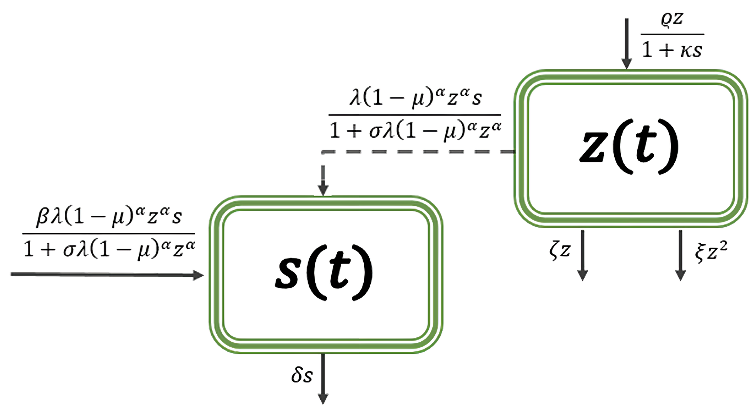
- We consider the type IV functional response, and it is nondifferentiable on the s-axis. The functional response ultimately increases (when ) as the efficiency of aggregation for prey increases and it decreases as the refuge capacity increases.
- The predator population falls into decay if the per capita death rate of the predator is greater than a constant that depends on several parameters. Note that this decreases as the capacity of a refuge at t increases, and increases (decreases) as the value of the efficiency of aggregation for prey increases if ().
- Because of the term, the Jacobian matrix is indeterminate at the origin. Therefore, it is impossible to carry out a stability analysis by merely looking at its eigenvalues. We use the definition of stability to prove that if , then is stable, and if , then is unstable.
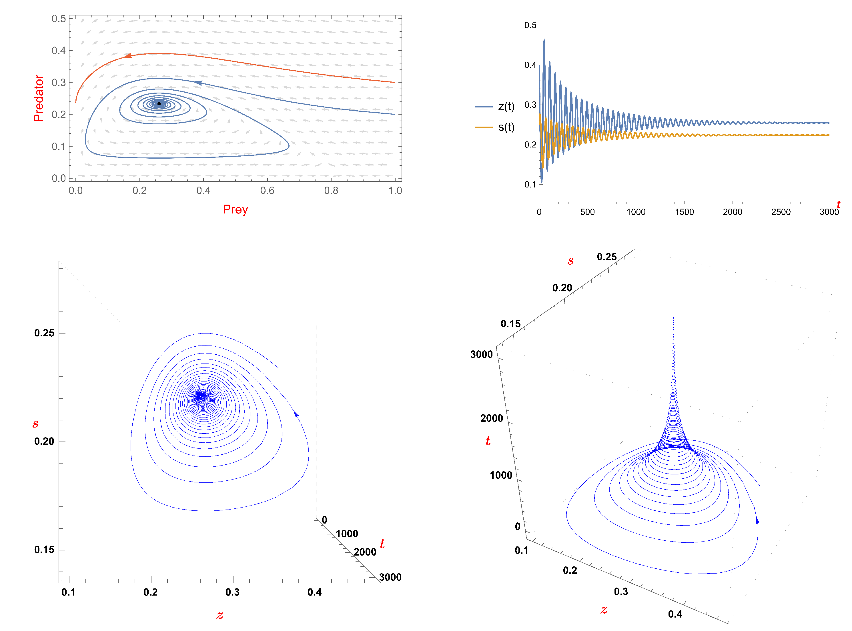
- Under some conditions, the coexistence state of system (5) is stable and the alteration in the fear factor’s value has no bearing on this stability.
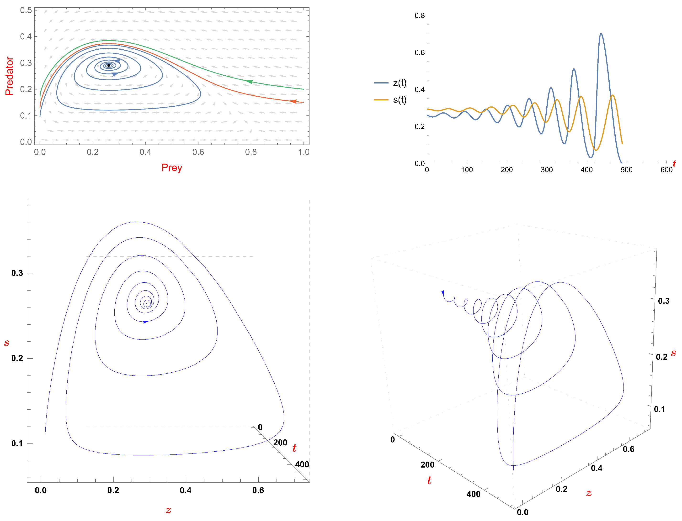
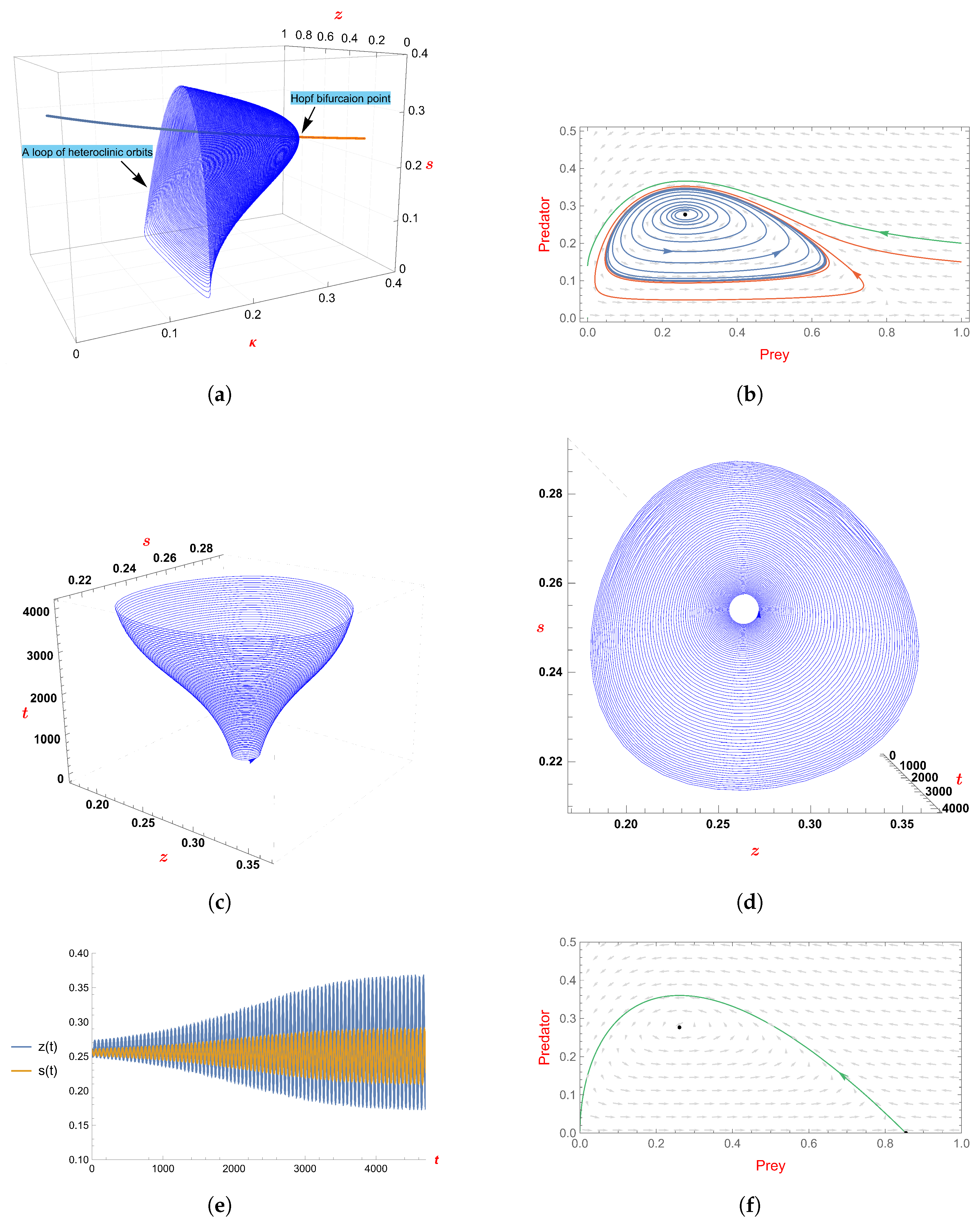
- We examine the Hopf bifurcation at the unique positive equilibrium. When the fear factor’s value decreases, the limit cycle appears when the fear factor’s value is less than , and it disappears when the fear factor’s value is equal to through a loop of heteroclinic orbits.
2. Boundedness and Positivity
3. Non-Persistence
4. Steady States and Their Stability
4.1. The Trivial Steady State

4.2. The Predator-Free Steady State
- (i)
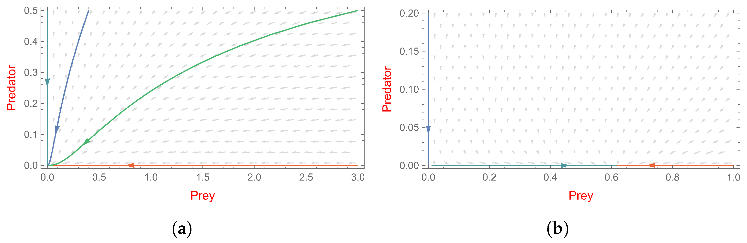
- Assuming that and hold, then is a stable node.
- (ii)
- Assuming that and hold, then is an unstable saddle point.
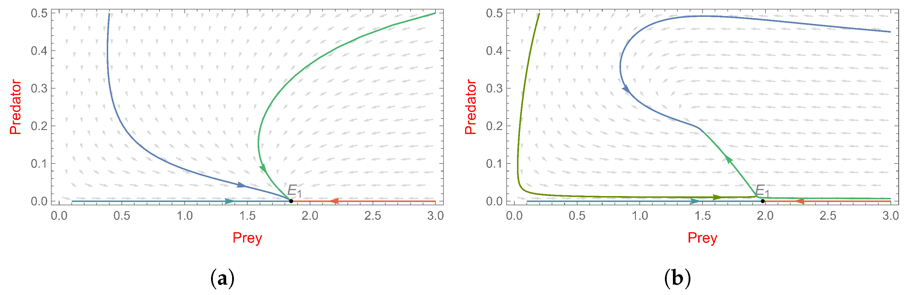
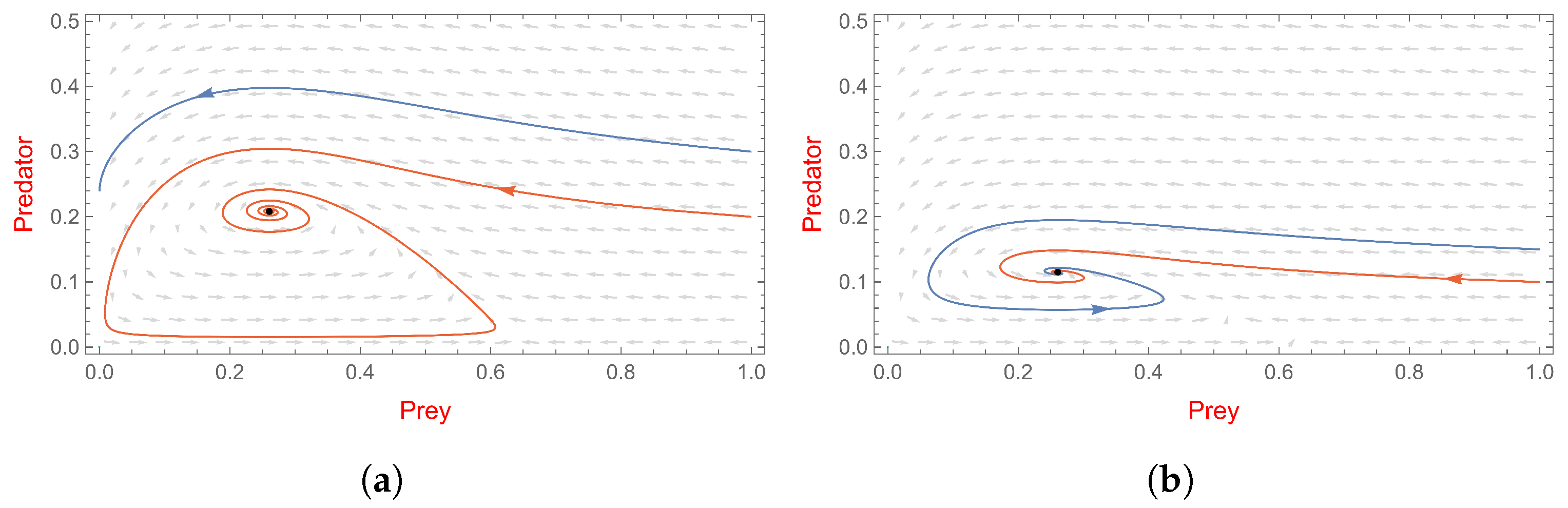
- , system (2) has a non-trivial boundary equilibrium ;
- and is a stable node (see Figure 4a).
- , system (3) has a non-trivial boundary equilibrium ;
- and is an unstable saddle point (see Figure 4b).
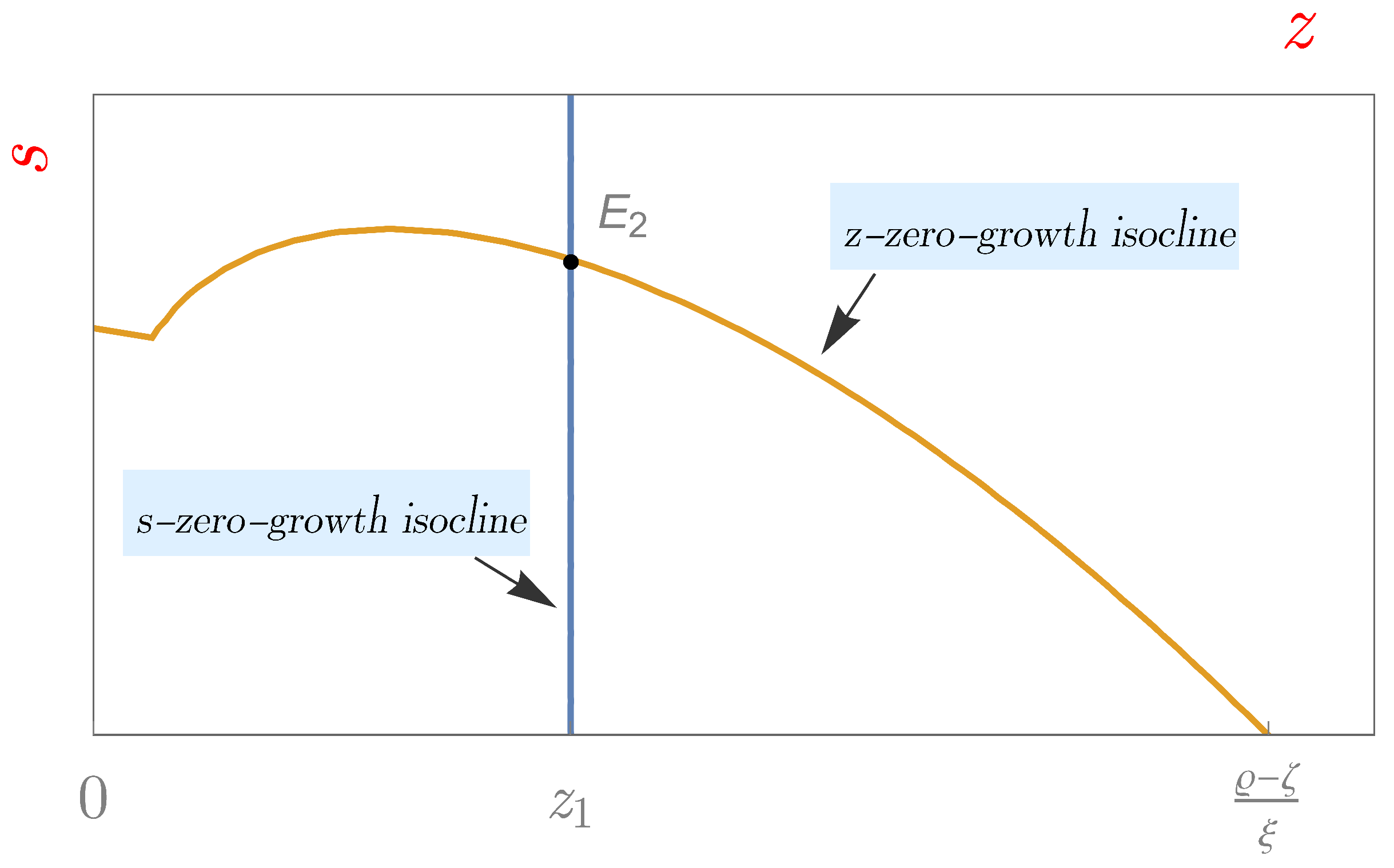
4.3. The Steady State of Coexistence
5. The Effect of Fear
- 1.
- If a() > 0, the bifurcation periodic solution is unstable, and it is bifurcating from as κ increases and passes .
- 2.
- If a() < 0, the bifurcation periodic solution is orbitally asymptotically stable, and it is bifurcating from as κ decreases and passes .
6. Direction of Hpof Bifurcation with as Bifurcation Parameter
7. Examples and Simulations
8. Discussion
- According to Theorem 2, when , the predator population is non-persistent, i.e., the predator population falls into decay if the per capita death rate of the predator is greater than a constant that depends on several parameters. Note that this decreases as the capacity of a refuge at t increases, and increases (decreases) as the value of the efficiency of aggregation for prey increases if ().
- Because of the term, the Jacobian matrix is indeterminate at the origin. Therefore, it is impossible to carry out a stability analysis by simply looking at its eigenvalues. We used the definition of stability to prove that if , then is stable, and if , then is unstable.
- If , the coexistence state of system (5) is stable and the alteration in the fear factor’s value has no bearing on this stability.
- If , we examine the Hopf bifurcation at the unique positive equilibrium. When the fear factor’s value decreases, the limit cycle appears when the fear factor’s value is less than , and it disappears when the fear factor’s value is equal to through a loop of heteroclinic orbits.
Author Contributions
Funding
Data Availability Statement
Conflicts of Interest
References
- Sadava, D.E.; Hillis, D.M.; Heller, H.C. Life: The Science of Biology; Macmillan: Stuttgart, Germany, 2009; Volume 2. [Google Scholar]
- Li, Y.; Wang, J. Spatiotemporal patterns of a predator–prey system with an allee effect and holling type iii functional response. Int. J. Bifurc. Chaos 2016, 26, 1650088. [Google Scholar] [CrossRef]
- Wang, J.; Wei, J. Bifurcation analysis of a delayed predator–prey system with strong allee effect and diffusion. Appl. Anal. 2012, 91, 1219–1241. [Google Scholar] [CrossRef]
- Lv, Y.; Chen, L.; Chen, F.; Li, Z. Stability and bifurcation in an si epidemic model with additive allee effect and time delay. Int. J. Bifurc. Chaos 2021, 31, 2150060. [Google Scholar] [CrossRef]
- Lv, Y.; Chen, L.; Chen, F. Stability and bifurcation in a single species logistic model with additive allee effect and feedback control. Adv. Differ. Equations 2020, 2020, 1–15. [Google Scholar] [CrossRef] [Green Version]
- Wang, D. Positive periodic solutions for a nonautonomous neutral delay prey-predator model with impulse and hassell-varley type functional response. Proc. Am. Math. Soc. 2014, 142, 623–638. [Google Scholar] [CrossRef]
- Tang, X.; Song, Y. Cross-diffusion induced spatiotemporal patterns in a predator–prey model with herd behavior. Nonlinear Anal. Real World Appl. 2015, 24, 36–49. [Google Scholar] [CrossRef]
- Tang, X.; Song, Y.; Zhang, T. Turing–hopf bifurcation analysis of a predator–prey model with herd behavior and cross-diffusion. Nonlinear Dyn. 2016, 86, 73–89. [Google Scholar] [CrossRef]
- Yuan, S.; Xu, C.; Zhang, T. Spatial dynamics in a predator-prey model with herd behavior. Chaos Interdiscip. J. Nonlinear Sci. 2013, 23, 033102. [Google Scholar] [CrossRef]
- Song, Y.; Tang, X. Stability, steady-state bifurcations, and turing patterns in a predator–prey model with herd behavior and prey-taxis. Stud. Appl. Math. 2017, 139, 371–404. [Google Scholar] [CrossRef]
- Song, Y.; Wu, S.; Wang, H. Spatiotemporal dynamics in the single population model with memory-based diffusion and nonlocal effect. J. Differ. Equations 2019, 267, 6316–6351. [Google Scholar] [CrossRef]
- Wang, J.; Shi, J.; Wei, J. Nonexistence of periodic orbits for predator-prey system with strong allee effect in prey populations. Electron. J. Differ. Equations 2013, 2013, 1–14. [Google Scholar]
- Jeschke, J.M.; Kopp, M.; Tollrian, R. Consumer-food systems: Why type i functional responses are exclusive to filter feeders. Biol. Rev. 2004, 79, 337–349. [Google Scholar] [CrossRef] [PubMed]
- Holling, C.S. Some characteristics of simple types of predation and parasitism1. Can. Entomol. 1959, 91, 385–398. [Google Scholar] [CrossRef]
- DeLong, J.P. Predator Ecology: Evolutionary Ecology of the Functional Response; Oxford University Press: Oxford, UK, 2021. [Google Scholar]
- Köhnke, M.C.; Siekmann, I.; Seno, H.; Malchow, H. A type iv functional response with different shapes in a predator–prey model. J. Theor. Biol. 2020, 505, 110419. [Google Scholar] [CrossRef] [PubMed]
- Creel, S.; Christianson, D. Relationships between direct predation and risk effects. Trends Ecol. Evol. 2008, 23, 194–201. [Google Scholar] [CrossRef]
- Lima, S.L. Nonlethal effects in the ecology of predator-prey interactions. Bioscience 1998, 48, 25–34. [Google Scholar] [CrossRef] [Green Version]
- Lima, S.L. Predators and the breeding bird: Behavioral and reproductive flexibility under the risk of predation. Biol. Rev. 2009, 84, 485–513. [Google Scholar] [CrossRef]
- Cresswell, W. Predation in bird populations. J. Ornithol. 2011, 152, 251–263. [Google Scholar] [CrossRef]
- Zanette, L.Y.; White, A.F.; Allen, M.C.; Clinchy, M. Perceived predation risk reduces the number of offspring songbirds produce per year. Science 2011, 334, 1398–1401. [Google Scholar] [CrossRef]
- Preisser, E.L.; Bolnick, D.I. The many faces of fear: Comparing the pathways and impacts of nonconsumptive predator effects on prey populations. PLoS ONE 2008, 3, e2465. [Google Scholar] [CrossRef] [Green Version]
- Xie, B.; Zhang, Z.; Zhang, N. Influence of the fear effect on a holling type ii prey–predator system with a michaelis–menten type harvesting. Int. J. Bifurc. Chaos 2021, 31, 2150216. [Google Scholar] [CrossRef]
- Pal, S.; Pal, N.; Samanta, S.; Chattopadhyay, J. Effect of hunting cooperation and fear in a predator-prey model. Ecol. Complex. 2019, 39, 100770. [Google Scholar] [CrossRef]
- Pal, S.; Majhi, S.; Mandal, S.; Pal, N. Role of fear in a predator–prey model with beddington–deangelis functional response. Z. Naturforschung A 2019, 74, 581–595. [Google Scholar] [CrossRef]
- Zhang, H.; Cai, Y.; Fu, S.; Wang, W. Impact of the fear effect in a prey-predator model incorporating a prey refuge. Appl. Math. Comput. 2019, 356, 328–337. [Google Scholar] [CrossRef]
- Yu, F.; Wang, Y. Hopf bifurcation and bautin bifurcation in a prey–predator model with prey’s fear cost and variable predator search speed. Math. Comput. Simul. 2022, 196, 192–209. [Google Scholar] [CrossRef]
- Lai, L.; Zhu, Z.; Chen, F. Stability and bifurcation in a predator–prey model with the additive allee effect and the fear effect. Mathematics 2020, 8, 1280. [Google Scholar] [CrossRef]
- Li, Y.; He, M.; Li, Z. Dynamics of a ratio-dependent leslie–gower predator–prey model with allee effect and fear effect. Math. Comput. Simul. 2022, 201, 417–439. [Google Scholar] [CrossRef]
- Sasmal, S.K.; Takeuchi, Y. Dynamics of a predator-prey system with fear and group defense. J. Math. Anal. Appl. 2020, 481, 123471. [Google Scholar] [CrossRef]
- Wang, X.; Zanette, L.; Zou, X. Modelling the fear effect in predator–prey interactions. J. Math. Biol. 2016, 73, 1179–1204. [Google Scholar] [CrossRef]
- Dugatkin, L.A. Cooperation among Animals: An Evolutionary Perspective; Oxford University Press on Demand: Oxford, UK, 1997. [Google Scholar]
- Prins, H. Buffalo herd structure and its repercussions for condition of individual african buffalo cows. Ethology 1989, 81, 47–71. [Google Scholar] [CrossRef]
- Partridge, B.L.; Johansson, J.; Kalish, J. The structure of schools of giant bluefin tuna in cape cod bay. Environ. Biol. Fishes 1983, 9, 253–262. [Google Scholar] [CrossRef]
- Elder, W.H.; Elder, N.L. Role of the family in the formation of goose flocks. Wilson Bull. 1949, 61, 132–140. [Google Scholar]
- Wilsdon, C. Animal Defenses; Infobase Publishing: New York, NY, USA, 2014. [Google Scholar]
- Ajraldi, V.; Pittavino, M.; Venturino, E. Modeling herd behavior in population systems. Nonlinear Anal. Real World Appl. 2011, 12, 2319–2338. [Google Scholar] [CrossRef]
- Venturino, E.; Petrovskii, S. Spatiotemporal behavior of a prey–predator system with a group defense for prey. Ecol. Complex. 2013, 14, 37–47. [Google Scholar] [CrossRef] [Green Version]
- Djilali, S. Impact of prey herd shape on the predator-prey interaction. Chaos Solitons Fractals 2019, 120, 139–148. [Google Scholar] [CrossRef]
- Bulai, I.M.; Venturino, E. Shape effects on herd behavior in ecological interacting population models. Math. Comput. Simul. 2017, 141, 40–55. [Google Scholar] [CrossRef]
- Tang, B. Dynamics for a fractional-order predator-prey model with group defense. Sci. Rep. 2020, 10, 1–17. [Google Scholar] [CrossRef] [Green Version]
- Xu, C.; Yuan, S.; Zhang, T. Global dynamics of a predator–prey model with defense mechanism for prey. Appl. Math. Lett. 2016, 62, 42–48. [Google Scholar] [CrossRef]
- Du, Y.; Niu, B.; Wei, J. A predator-prey model with cooperative hunting in the predator and group defense in the prey. Discret. Contin. Dyn. Syst. B 2022, 27, 5845. [Google Scholar] [CrossRef]
- Djilali, S.; Mezouaghi, A.; Belhamiti, O. Bifurcation analysis of a diffusive predator-prey model with schooling behaviour and cannibalism in prey. Int. J. Math. Model. Numer. 2021, 11, 209–231. [Google Scholar] [CrossRef]
- Belabbas, M.; Ouahab, A.; Souna, F. Rich dynamics in a stochastic predator-prey model with protection zone for the prey and multiplicative noise applied on both species. Nonlinear Dyn. 2021, 106, 2761–2780. [Google Scholar] [CrossRef]
- Souna, F.; Lakmeche, A. Spatiotemporal patterns in a diffusive predator–prey system with leslie–gower term and social behavior for the prey. Math. Methods Appl. Sci. 2021, 44, 13920–13944. [Google Scholar] [CrossRef]
- Ye, Y.; Zhao, Y. Bifurcation analysis of a delay-induced predator–prey model with allee effect and prey group defense. Int. J. Bifurc. Chaos 2021, 31, 2150158. [Google Scholar] [CrossRef]
- Meng, X.Y.; Meng, F.L. Bifurcation analysis of a special delayed predator-prey model with herd behavior and prey harvesting. AIMS Math. 2021, 6, 5695–5719. [Google Scholar] [CrossRef]
- Mezouaghi, A.; Djilali, S.; Bentout, S.; Biroud, K. Bifurcation analysis of a diffusive predator–prey model with prey social behavior and predator harvesting. Math. Methods Appl. Sci. 2022, 45, 718–731. [Google Scholar] [CrossRef]
- Bainov, D.D.; Simeonov, P.S. Integral Inequalities and Applications; Springer Science & Business Media: Berlin/Heidelberg, Germany, 2013; Volume 57. [Google Scholar]
- Wiggins, S.; Golubitsky, M. Introduction to Applied Nonlinear Dynamical Systems and Chaos; Springer: Berlin, Germany, 2003; Volume 2. [Google Scholar]
- Abell, M.L.; Braselton, J.P. Differential Equations with Mathematica; Academic Press: Cambridge, MA, USA, 2022. [Google Scholar]


| Symbol | Interpretation | Assumptions |
|---|---|---|
| z | Prey density | |
| s | Predator density | |
| Number of prey successfully attacked per predator | , | |
| Prey population birth rate | ||
| Rate of natural mortality in prey populations | ||
| Mortality rate as a result of interspecies competition | ||
| Level of fear | ||
| Capacity of a refuge at t | ||
| Attack rate per predator and prey | ||
| Prey conversion to the predator | ||
| Per capita death rate of the predator | ||
| Efficiency of aggregation for prey | ||
| Handling time per prey | ||
| Incipient limiting level |
Disclaimer/Publisher’s Note: The statements, opinions and data contained in all publications are solely those of the individual author(s) and contributor(s) and not of MDPI and/or the editor(s). MDPI and/or the editor(s) disclaim responsibility for any injury to people or property resulting from any ideas, methods, instructions or products referred to in the content. |
© 2023 by the authors. Licensee MDPI, Basel, Switzerland. This article is an open access article distributed under the terms and conditions of the Creative Commons Attribution (CC BY) license (https://creativecommons.org/licenses/by/4.0/).
Share and Cite
Al-Mohanna, S.M.G.; Xia, Y.-H. Fear Effect on a Predator–Prey Model with Non-Differential Fractional Functional Response. Fractal Fract. 2023, 7, 312. https://doi.org/10.3390/fractalfract7040312
Al-Mohanna SMG, Xia Y-H. Fear Effect on a Predator–Prey Model with Non-Differential Fractional Functional Response. Fractal and Fractional. 2023; 7(4):312. https://doi.org/10.3390/fractalfract7040312
Chicago/Turabian StyleAl-Mohanna, Salam Mohammed Ghazi, and Yong-Hui Xia. 2023. "Fear Effect on a Predator–Prey Model with Non-Differential Fractional Functional Response" Fractal and Fractional 7, no. 4: 312. https://doi.org/10.3390/fractalfract7040312