Article

Finite-Time Synchronization for Fractional Order Fuzzy Inertial Cellular Neural Networks with Piecewise Activations and Mixed Delays

1
School of Computer Science, Huainan Normal University, Huainan 232038, China
2
School of Finance and Mathematics, Huainan Normal University, Huainan 232038, China
*
Author to whom correspondence should be addressed.
Fractal Fract. 2023, 7(4), 294; https://doi.org/10.3390/fractalfract7040294
Submission received: 5 February 2023 / Revised: 10 March 2023 / Accepted: 26 March 2023 / Published: 29 March 2023
(This article belongs to the Special Issue Robust and Adaptive Control of Fractional-Order Systems)

Abstract

:
This paper investigates a class of finite-time synchronization problems of fractional order fuzzy inertial cellular neural networks (FFICNNs) with piecewise activations and mixed delays. First, the Caputo FFICNNs are established. A suitable transformation variable is constructed to rewrite FFICNNs with mixed delays into a first-order differential system. Secondly, some new effective criteria are constructed on the basis of the finite-time stability theory and Lyapunov functionals to realize the synchronization of the drive-response system. Finally, two numerical simulation examples show that the proposed method is effective.

1. Introduction

Yang et al. [1,2] put forward cellular neural networks (CNNs) in 1988, which have since been extensively investigated and applied in such fields as secondary optimization, pattern classification, pattern recognition, associative memory, and image processing. Yang et al. [3] put forward the fuzzy cellular neural networks (FCNNs) in 1996. Compared with the CNNs, the FCNNs contains fuzzy logics, and there is a local connection between cells [4,5,6,7,8,9,10]. FCNNs have superior performance applications in image encryption, psychophysics, perception, robots, secure communication, and medical diagnosis, etc.
Babcock et al. [11] supplemented an inertial term to neural networks to make up inertial neural networks (INNs) in 1986, which caused more complex bifurcation and chaotic dynamic behaviors of neuron coupling as instability and concussion behaviors. Adding an inertia term to electronic neural networks may bring about complex behaviors such as spontaneous concussion, instability, and chaotic behavior. Moreover, there exist significant biological backgrounds for bringing the inertial term into neural systems. Many researchers have paid extensive attention to inertial neural networks, and have made important progress (see [12,13,14,15,16]).
Fractional order calculus is an extension of integer calculus to arbitrary order, has become a mathematical tool to solve practical problems in pattern recognition, information processing, robot control, physics, statistics, and other fields for its superiority, which is characterized by infinite memory considering the current states and all its previous ones. Scholars [17,18,19,20,21,22] used fractional operators to build fractional order neural network models.
In practical application, the signals of processing and transmission between neurons are limited by the switching speed of the amplifier, the delay time is inevitable, and this will influence the stability of the neural networks and give rise to divergence, instability, and oscillation in network systems. In fact, mixed delays include constant ones, time-varying ones, and distributed ones, which are considered to be more effective than single ones at modeling network systems in that these simple delays are often impractical, while network systems become more complex.
Synchronization is the dynamic behavior of the drive system and reponse system to attain the same state after a certain time. Nowadays, much attention has been paid to synchronization, owing to its potential applications in medicine, information science, optimized calculation, automatic control, and other fields. At present, there are many achievements in synchronous research. According to the convergence time, it is mainly divided into three categories: global asymptotical synchronization, exponential synchronization, and finite-time synchronization. In comparison with the global asymptotical synchronization of neural networks, finite-time synchronization has better convergence performance. However, the final convergence time is closely related to the initial state of the drive-response system. To achieve synchronization quickly, we can rely on control methods—for example, feedback control, adaptive control, intermittent control, etc. Of course, we sincerely hope that systems can achieve synchronization with practical engineering applications in a finite time. Therefore, the research for finite-time synchronization of neural networks is of great significance. At present, the research result of the inertial neural networks’ synchronization mainly includes the following aspects. Yang et al. [23] designed three different types of controllers by using the maximum analysis method to ensure the global asymptotic synchronization between the drive-response system. Feng et al. [24] investigated the exponential synchronization control of inertial neural networks with time-varying delays. By designing Lyapunov–Krasovskii functionals and utilizing new weighted integral inequalities, the delay-related criteria of linear matrix inequality (LMI) are obtained. Zhang et al. [25] obtained two new strategies to solve the synchronization for fractional neural networks with two inertia terms and a time delay by constructing Lyapunov function and using the LMI method. Tang et al. [26] researched the exponential synchronization of INNs with finite and discrete distributed mixed delays by using intermittent control. Liang et al. [27] introduced the exponential synchronization control of inertial Cohen–Grossberg neural networks with time-varying delays. Shi et al. [28] studied the lag synchronization and global exponential stabilization of INNs via adaptive control by constructing nonnegative function and employing inequality techniques, and obtained several new results. Zhang et al. [29] introduced the finite-time synchronization control of FINNs with the maximum method of functions. Hua et al. [30] introduced a new control method to solve the finite-time synchronization problem of IMNNs with time-varying delay. It can effectively dispose of the problems caused by mixed delay and memristor connection weight. Chen et al. [31] design four different kinds of feedback controllers, under which the considered inertial memristive neural networks can realize fixed-time synchronization perfectly. Alimi et al. [32] introduced the finite/fixed time synchronization of the INNs with multiple proportional delays. Yang et al. [33] studies the synchronization control of a new FICNNs with piecewise activation and mixed delay. However, few reports are found in the existing works for finite-time synchronization of FFICNNs with piecewise activation and mixed delay.
Motivated by these, this paper will investigate the problems of finite-time synchronization analysis for a class of FFICNNs with piecewise activation and mixed delay. There are the following primary innovations in this paper.
  • The Caputo fractional order fuzzy inertial cellular neural networks model is established. It can be used to describe many systems of internal coherence in the real environment. In addition, it is easy to implement in engineering applications and has important application prospects.
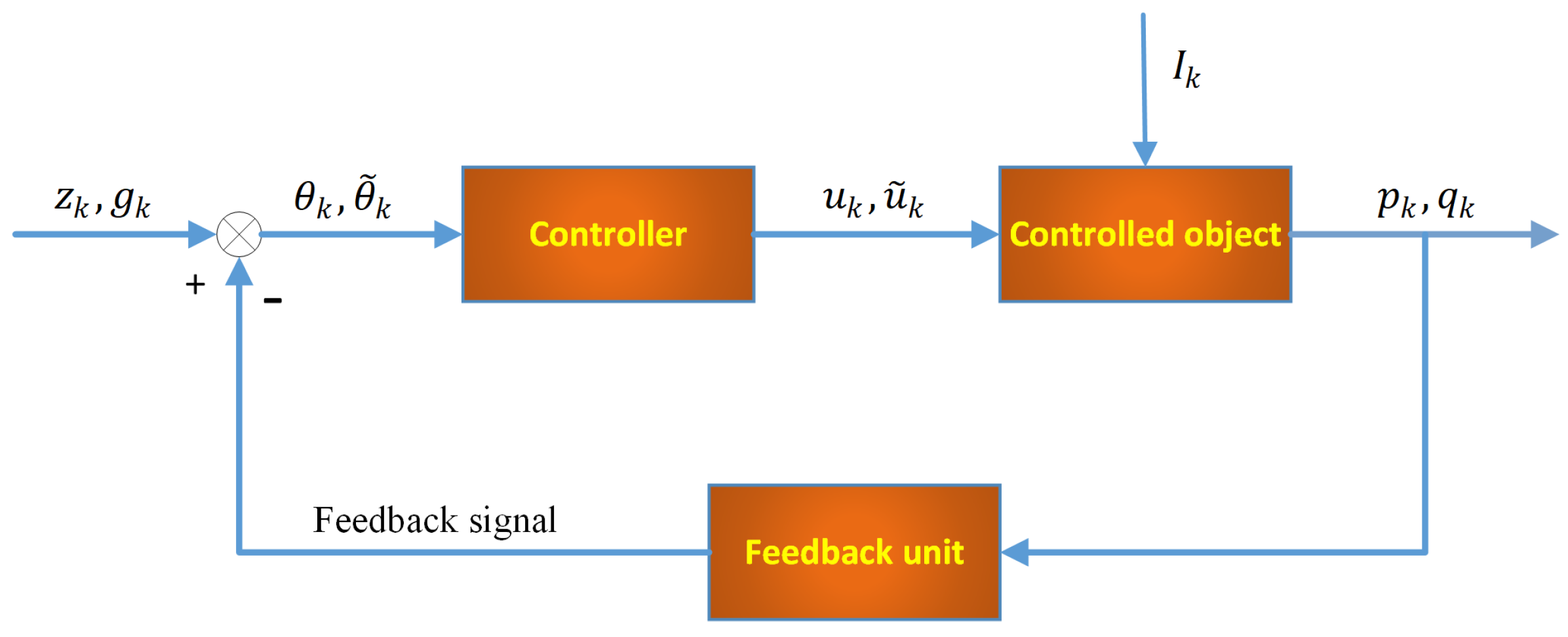
  • A novel nonlinear controller is designed to realize the finite-time synchronization of FFICNNs with piecewise activation and mixed delay. It is of high reliability and great accuracy, and can better synchronize the position and motion of the system.
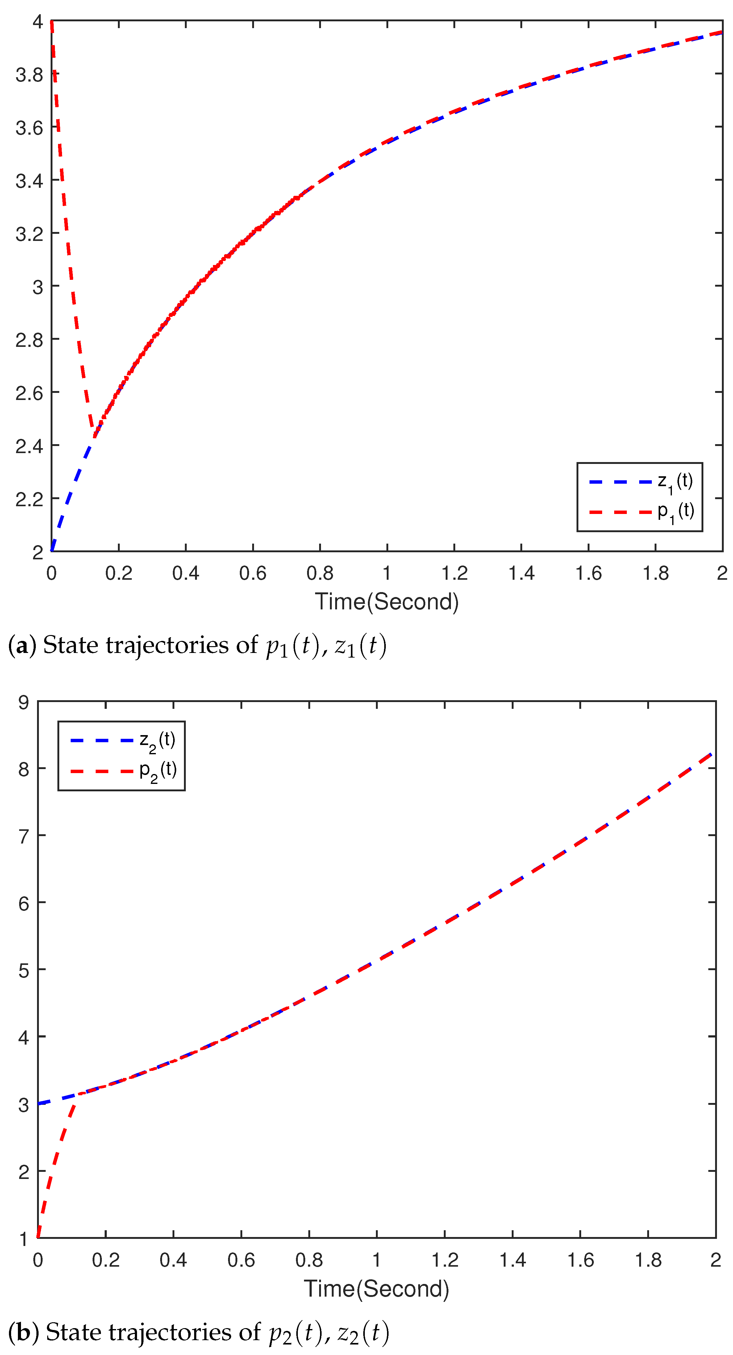
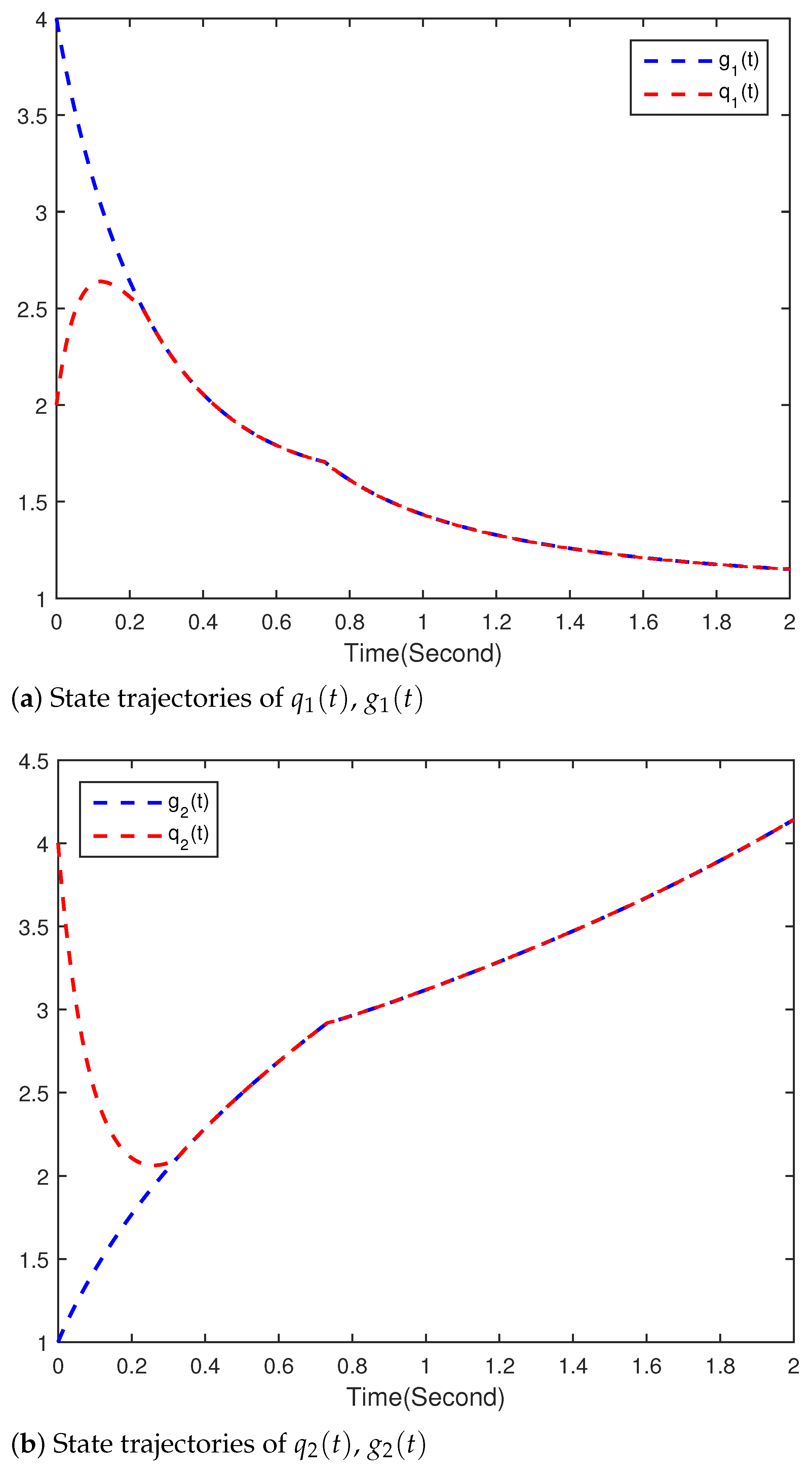
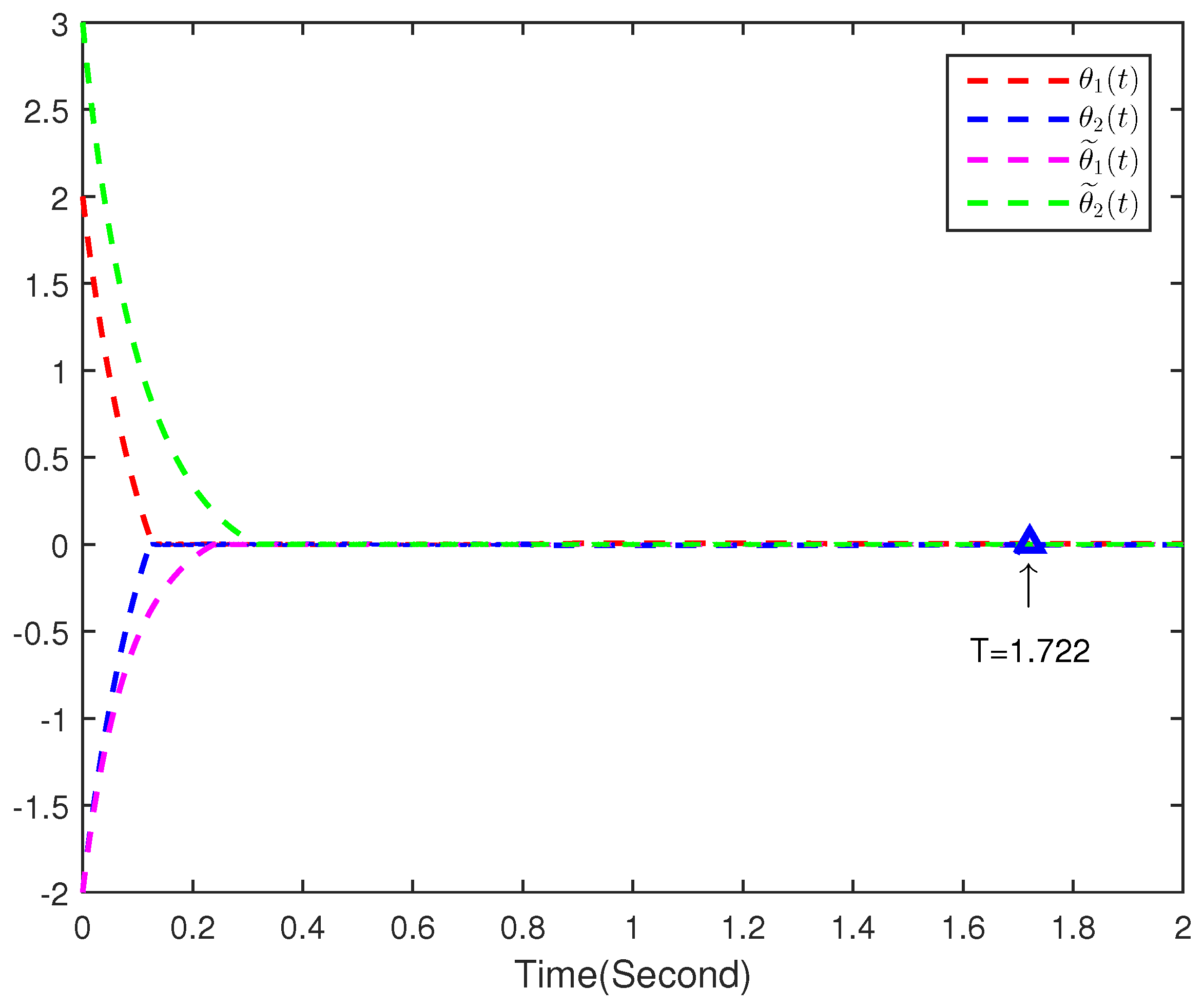
  • The Lyapunov direct method is applied in the analysis of the inertial system to avoid the loss of the inertia. The numerical simulation results show that the designed method is effective. Therefore, it is of more important practical significance.
The other parts of this paper are structured as follows. Section 2 introduces the network system model of FICNNs with piecewise activations and mixed delays, assumptions, lemmas, and definitions of finite-time synchronization. In Section 3, the synchronization of the neural network system is analyzed. In Section 4, two examples are given to demonstrate the effectiveness of the obtained results. The conclusion is revealed in Section 5.

2. Preliminaries and Problem Formulation

2.1. Preliminaries

In this article, the system model is defined by Caputo fractional order. First, some basic definitions, lemmas, and assumptions about fractional calculus are introduced.
Definition 1
([34]). By using Equation (1) to define the fractional integral of the function z ( t ) , we have
t 0 C D t α z ( t ) = 1 Γ ( α ) t 0 t ( t x ) α 1 z ( x ) d x ,
where α > 0 , t > t 0 , Γ ( · ) is gamma function.
Definition 2
([34]). By using Equation (2) to define the the fractional derivative of the function z ( t ) , we have
t 0 C D t α z ( t ) = 1 Γ ( n α ) t 0 t ( t x ) n α 1 z ( n ) ( x ) d x ,
where t > t 0 , α ( m 1 , m ] , m Z + . If α ( 0 , 1 ] , then
t 0 C D t α z ( t ) = 1 Γ ( 1 α ) t 0 t z ( x ) ( t x ) α d x .
For simplicity, we use D t α z ( t ) to represent 0 C D t α z ( t ) in this article. Some useful lemmas are given as follows.
Lemma 1
([35]). Suppose that z ( t ) C 1 [ 0 , T ] , T > 0 and β ( 0 , 1 ] , and then Equation (4) holds,
D t β D t β z ( t ) = z ( t ) z ( 0 )
and
D t β D t β z ( t ) = z ( t ) .
Lemma 2
([35]). Suppose that z ( t ) C n [ 0 , T ] , T > 0 , and then Equation (6) holds,
D t β z ( t ) = D t β m · · · D t β 2 D t β 1 z ( t ) ,
where t [ 0 , T ] , β = i = 1 m β i , β i ( 0 , 1 ] , n 1 < β n Z + , and there exist i l < m s.t. j = 1 i l β j = l ( l = 1 , 2 , · · · , n 1 ).
Lemma 3
([36]). Suppose that a , b R , β > 0 , and then Equation (7) holds:
D t β ( a z 1 ( t ) + b z 2 ( t ) ) = a D t β z 1 ( t ) + b D t β z 2 ( t ) .
Lemma 4
([37]). Suppose that z ( t ) C 1 [ t 0 , ] , β ( 0 , 1 ] , and then Equation (8) holds:
D t β | z ( t ) | s i g n ( z ( t ) ) D t β z ( t ) .
Lemma 5
([38]). Suppose that function z ( t ) : [ 0 , + ] R m is differentiable and bounded, and β ( 0 , 1 ] , and then Equation (9) holds:
D t β z T ( t ) z ( t ) 2 z T ( t ) D t β z ( t ) .
Lemma 6
([3]). Suppose that a k r , b k r , x r , y r R , h r : R R are continuous functions for k , r = 1 , 2 , , m , and then Equation (10) holds:
| r = 1 m a k r h r ( x r ) r = 1 m a k r h r ( y r ) | r = 1 m | a k r | | h r ( x r ) h l ( y r ) | | r = 1 m b k r h r ( x r ) r = 1 m b k r h r ( y r ) | r = 1 m | b k r | | h r ( x r ) h r ( y r ) | .
Lemma 7
([39]). If a 1 , a 2 , , a m 0 , 0 < ν 1 , μ > 1 , then Equation (11) holds:
k = 1 m a k μ n 1 μ k = 1 m a k μ , k = 1 m a k ν k = 1 m a k ν .
Lemma 8
([40]). Suppose that V ( t ) is a nonnegative and continuous definite function, if it satisfies the inequality Equation (12), and then Equation (13) holds,
D t q V ( t ) c V η ( t )
V q η ( t ) V q η ( t 0 ) c Γ ( 1 + q η ) ( t t 0 ) q Γ ( 1 + q ) Γ ( 1 η ) , t [ t 0 , T ] ,
where c > 0 , η ( 0 , q ) , and q > 0 . T may be given by the following:
T = t 0 + Γ ( 1 + q ) Γ ( 1 η ) V q η ( t 0 ) c Γ ( 1 + q η ) 1 q .

2.2. Problem Formulation

In this paper, the system of the m-dimensional FFCNNs with piecewise activation and mixed delays is defined as
D t 2 α z k ( t ) = a k D t α z k ( t ) b k x k ( t ) + r = 1 m c k r h k ( z r ( t ) ) + r = 1 m d k r t σ 0 ( t ) t h r ( z r ( s ) ) d s + r = 1 m g k r v k + r = 1 m P k ν r + r = 1 m α k r h r ( z r ( t σ r ( t ) ) ) + r = 1 m Q k ν r + r = 1 m β k r h r ( z r ( t σ r ( t ) ) ) + I k z k ( ι ) = ψ k ( ι ) , D t α x k ( ι ) = φ k ( ι ) , ι [ σ , t 0 ] , k = 1 , , m ,
where 0 < α 1 . z k ( t ) represent the state of the kth neuron. a k , b k represent the passive decay rate to the state of kth neuron. c k r , d k r represent elements of feedback template and g k r denotes the feedforward template. v k and I k are input and bias of the kth neuron, respectively. α k r , β k r are fuzzy feedback MIN and MAX template, P k r , Q k r are fuzzy feedforward MIN and MAX template. h k ( · ) denotes activation functions, σ 0 ( t ) and σ k ( t ) represent the delay of the kth neuron.
Remark 1.
The mixed delay σ meets the following conditions: σ = max 0 r m { sup t R + σ r ( t ) } , ψ k ( s ) , φ k ( s ) C ( [ σ , t 0 ] , R m ) with C ( [ σ , t 0 ] , R m ) represents the Banach space of continuous functions [ σ , t 0 ] into R n . If the activation functions h k ( · ) is piecewise, it has a Filippov solution.
We assume that the following assumptions about activation functions are satisfied.
Assumption 1.
There exist nonnegative constants L k and S k such that
| λ k ζ k | L k | p k q k | + S k , p k , q k R , k = 1 , 2 , , m ,
where λ k c o ¯ [ h k ( p k ) ] and ζ k c o ¯ [ h k ( q k ) ] ; c o ¯ represents the convex closure of the set.
Assumption 2.
x i : R R is continuous except on a countable set of isolation points { ϱ k i } for each i = 1 , 2 , , n , where there exists a finite left limit x i ( ϱ k i ) and right limit x i ( ϱ k i + ) . Moreover, g i has at most a finite number of jump discontinuities in every compact interval of R.
Remark 2.
Assumptions 1 and 2 are not restrictive. Generally, the neural network model can satisfy Assumptions 1 and 2 in [41,42,43]. In addition, to obtain the main results, the concept of Filippov solution, which comes from Filippov for system (14), is given.
Definition 3.
If (i) and (ii) are satisfied, then the function z = ( z 1 , z 2 , , z m ) T is said to be a solution of system (14) on [ σ , T ) . Here, σ = max 0 r m { sup t R + σ r ( t ) } , T ( 0 , + ) .
(i) The function z = ( z 1 , z 2 , , z m ) T is continuous in the interval [ σ , T ) , and it is absolutely continuous in the interval [ 0 , T ) .
(ii) The λ = ( λ 1 , λ 2 , , λ m ) T : [ σ , T ) R m is a measurable function, such that λ l ( t ) c o ¯ [ h k ( z l ( t ) ) ] for t [ σ , T ] and
D t 2 α z k ( t ) = a k D t α z k ( t ) b k z k ( t ) + r = 1 m c k r λ r ( t ) + r = 1 m d k r t σ 0 ( t ) t λ r ( s ) d s + r = 1 m g k r v k + r = 1 m P k ν r + r = 1 m α k r λ r ( t σ r ( t ) ) + r = 1 m Q k ν r + r = 1 m β k r λ r ( t σ r ( t ) ) + I k , k = 1 , , m .
Let g k ( t ) = D t α z k ( t ) + ξ k z k ( t ) , where ξ k is constant. According to Lemmas 2 and 3, the system (16) can be transformed into the Equation (17), and it is chosen as the drive system. We have
D t α z k ( t ) = ξ k z k ( t ) + g k ( t ) D t α g k ( t ) = ϕ k g k ( t ) + δ k z k ( t ) + r = 1 m c k r λ r ( t ) + r = 1 m d k r t σ 0 ( t ) t λ r ( s ) d s + r = 1 m g k r v r + r = 1 m P k ν r + r = 1 m α k r λ r ( t σ r ( t ) ) + r = 1 m Q k ν r + r = 1 m β k r λ r ( t σ r ( t ) ) + I k , k = 1 , 2 , , m ,
where ϕ k = a k ξ k , δ k = ξ k 2 + ξ k a k b k , and Equation (18) is the initial value of system. We have
z k ( ι ) = ψ k ( ι ) g k ( ι ) = ξ k ψ k ( ι ) + φ k ( ι ) , ι [ σ , t 0 ] .
Now, we choose the system (19) as the response system. We have
D t α p k ( t ) = ξ k p k ( t ) + q k ( t ) + u k ( t ) D t α q k ( t ) = ϕ k q k ( t ) + δ k p k ( t ) + r = 1 m c k r ζ r ( t ) + r = 1 m d k r t σ 0 ( t ) t ζ r ( s ) d s + r = 1 m g k r v r + r = 1 m P k ν r + r = 1 m α k r ζ r ( t σ r ( t ) ) + r = 1 m Q k ν r + r = 1 m β k r ζ r ( t σ r ( t ) ) + I k + u ˜ k ( t ) , k = 1 , 2 , , m ,
where u ˜ k ( t ) , u k ( t ) represent the designed controller. Equation (20) is the error system:
θ k ( t ) = p k ( t ) z k ( t ) θ ˜ k ( t ) = q k ( t ) g k ( t ) .
According to Equation (17) and Equation (19), we obtain
D t α θ k ( t ) = ξ k θ k ( t ) + θ ˜ k ( t ) + u k ( t ) D t α θ ˜ k ( t ) = ϕ k θ ˜ k ( t ) + δ k θ k ( t ) + r = 1 m c k r ζ r ( t ) r = 1 m c k r λ r ( t ) + r = 1 m d k r t σ 0 ( t ) t ζ r ( s ) d s r = 1 m d k r t σ 0 ( t ) t λ r ( s ) d s + r = 1 m α k r ζ r ( t σ r ( t ) ) r = 1 m α k r λ r ( t σ r ( t ) ) + r = 1 m β k r ζ r ( t σ r ( t ) ) r = 1 m β k r λ r ( t σ r ( t ) ) + u ˜ k ( t ) , k = 1 , 2 , , m .
The structure of this FICNN is shown in Figure 1.
Definition 4
([32]). The drive system(17) and response systems (19) are synchronized within a finite time, if T > t 0 exists under properly designed controllers u ˜ k ( t ) , u k ( t ) , such that
lim t T p k ( t ) z k ( t ) = lim t T q k ( t ) g k ( t ) = 0
and p k ( t ) z k ( t ) = q k ( t ) g k ( t ) = 0 for all t > T , k = 1 , 2 , , m .

3. Finite-Time Synchronization

In this section, we will design controller u k ( t ) , u ˜ k ( t ) to get the finite-time synchronization between the drive-response systems. The controller is designed,
u k ( t ) = ρ s i g n θ k ( t ) | θ k ( t ) | μ + ω k | θ k ( t σ k ( t ) ) | k k θ k ( t ) u ˜ k ( t ) = s i g n θ ˜ k ( t ) η k 2 + ρ | θ ˜ k ( t ) | μ η k 1 θ ˜ k ( t ) r = 1 m d k r t σ 0 ( t ) t ζ r ( s ) d s t σ 0 ( t ) t λ r ( s ) d s , ,
where 0 < μ < 1 , ρ > 0 , k k , ω k , η k 1 , a n d η k 2 are the control parameters.
Theorem 1.
Assumptions 1 and 2 are true if the following conditions (23) hold; then, the system (17) and (19) can achieve finite-time synchronization under controller (22). We have
η k 1 1 ϕ k η k 2 r = 1 m | α k r | + | β k r | + | c k r | S r k k r = 1 m | c r k | L k + δ k ξ k ω k r = 1 m | α k r | + | β k r | L k
for k = 1 , 2 , , m . Furthermore, the T can be calculated by Equation (24),
T = t 0 + Γ ( 1 + α ) Γ ( 1 μ ) V α μ ( t 0 ) c Γ ( 1 + α μ ) 1 α ,
where
V ( t 0 ) = k = 1 m | θ k ( t 0 ) | + k = 1 m | θ ˜ k ( t 0 ) | .
Proof. 
Select the following Lyapunov function:
V ( t ) = k = 1 m | θ k ( t ) | + k = 1 m | θ ˜ k ( t ) | .
According to Lemmas 3 and 4, the derivative of V ( t ) is calculated, and we obtain
D t α V ( t ) k = 1 m s i g n θ k ( t ) D t α θ k ( t ) + k = 1 m s i g n θ ˜ k ( t ) D α θ ˜ k ( t ) = k = 1 m s i g n θ k ( t ) ξ k θ k ( t ) + θ ˜ k ( t ) + u k ( t ) + k = 1 m s i g n θ ˜ k ( t ) ( ϕ k θ ˜ k ( t ) + δ k θ k ( t ) + r = 1 m c k r ζ r ( t ) r = 1 m c k r λ r ( t ) + r = 1 m d k r t σ 0 ( t ) t ζ r ( s ) d s r = 1 m d k r t σ 0 ( t ) t λ r ( s ) d s + r = 1 m α k r ζ r ( t σ r ( t ) ) r = 1 m α k r λ r ( t σ r ( t ) ) + r = 1 m β k r ζ r ( t σ r ( t ) ) r = 1 m β k r λ r ( t σ r ( t ) ) + u ˜ k ( t ) ) .
Substituting the controller (22) into Equation (26), and we have
D t α V ( t ) k = 1 m s i g n θ k ( t ) ( ξ k θ k ( t ) + θ ˜ k ( t ) k k θ k ( t ) s i g n θ k ( t ) ( ρ | θ k ( t ) | μ + ω k | θ k ( t σ k ( t ) ) | ) ) + k = 1 m s i g n θ ˜ k ( t ) ( ϕ k θ ˜ k ( t ) + δ k θ k ( t ) + r = 1 m c k r ζ r ( t ) r = 1 m c k r λ r ( t ) + r = 1 m d k r t σ 0 ( t ) t ζ r ( s ) d s r = 1 n d k r t σ 0 ( t ) t λ r ( s ) d s + r = 1 m α k r ζ r ( t σ r ( t ) ) r = 1 m α k r λ r ( t σ r ( t ) ) + r = 1 m β k r ζ k ( t σ r ( t ) ) r = 1 m β k r λ r ( t σ r ( t ) ) η k 1 θ ˜ k ( t ) s i g n θ ˜ k ( t ) η k 2 + ρ | θ ˜ k ( t ) | μ r = 1 m d k r t σ 0 ( t ) t ζ r ( s ) d s + r = 1 m d k r t σ 0 ( t ) t λ r ( s ) d s ) ,
which yields
D t α V ( t ) k = 1 m ξ k k k + δ k | θ k ( t ) | + k = 1 m 1 + ϕ k η k 1 | θ ˜ k ( t ) | k = 1 m ω k | θ k ( t σ k ( t ) ) | k = 1 m ρ | θ k ( t ) | μ k = 1 m η k 1 + ρ | θ ˜ k ( t ) | μ + k = 1 m | r = 1 m α k r ζ r ( t σ r ( t ) ) r = 1 m α k r λ r ( t σ r ( t ) ) | + k = 1 m | r = 1 m β k r ζ r ( t σ r ( t ) ) r = 1 m β k r λ r ( t σ r ( t ) ) | + k = 1 m r = 1 m | c k r | | ζ r ( t ) λ l ( t ) | .
According to Assumption 1, we have
k = 1 m r = 1 m | c k r | | ζ r ( t ) λ r ( t ) | k = 1 m r = 1 m | c k r | L r | θ r ( t ) | + S r = k = 1 m r = 1 m | c r k | L k | θ k ( t ) | + S k .
By using Assumption 1 and Lemma 6, we have
| r = 1 m α k r ζ r ( t σ r ( t ) ) r = 1 m α k r λ r ( t σ r ( t ) ) | k = 1 m | α k r | | ζ r ( t σ r ( t ) ) λ r ( t σ r ( t ) ) | r = 1 m | α r k | L r | θ r ( t σ r ( t ) ) | + S r .
Similarly,
| r = 1 m β k r ζ r ( t σ r ( t ) ) r = 1 m β k r λ r ( t σ r ( t ) ) | k = 1 m | β k r | | ζ r ( t σ r ( t ) ) λ r ( t σ r ( t ) ) | r = 1 m | β r k | L r | θ r ( t σ r ( t ) ) | + S r .
By using the above inequality, we have
D t α V ( t ) k = 1 m ξ k k k + δ k + r = 1 m | c r k L k | | θ k ( t ) | + k = 1 m 1 + ϕ k η k 1 | θ ˜ k ( t ) | + k = 1 m r = 1 m | α r k | + | β r k | L k ω k | θ k ( t σ k ( t ) ) | + k = 1 m r = 1 m | α k r | + | β k r | + | c k r | S r η k 2 k = 1 m c | θ k ( t ) | μ k = 1 m c | θ ˜ k ( t ) | μ .
By using Lemma 7, it follows that
D t α V ( t ) k = 1 m c | θ k ( t ) | μ k = 1 m c | θ ˜ k ( t ) | μ c k = 1 m | θ k ( t ) | + k = 1 m | θ ˜ k ( t ) | μ = c V μ ( t ) .
Therefore, the drive (17) and the response (19) system can achieve to synchronization in the finite-time by Lemma 8. ☐
Remark 3.
The finite-time synchronization of FFICNNs with piecewise activations and mixed delays is achieved by constructing a suitable controller in Theorem 1. However, the control laws u k ( t ) and u ˜ k ( t ) are not easily adaptive, and they must meet some special conditions. Therefore, we will optimize the applicable laws u k ( t ) and u ˜ k ( t ) to improve the feasibility.
The controller is redesigned as follows,
u k ( t ) = k k 1 θ k ( t ) k k 2 s i g n θ k ( t ) | θ k ( t ) | μ u ˜ k ( t ) = η k 1 θ ˜ k ( t ) s i g n θ ˜ k ( t ) ( η k 2 | θ ˜ k ( t ) | μ + ω k | θ k ( t σ k ( t ) ) | + r = 1 m L r | d k r | t σ 0 ( t ) t | θ r ( s ) | d s + ρ k ) ,
where 0 < μ < 1 , k k 1 , k k 2 , η k 1 , η k 2 , ρ k , ω k are the control parameters. Then we have the following theorem.
Theorem 2.
Assumptions 1 and 2 are true if the following conditions (29) hold, and then the system (17) and (19) can achieve finite-time synchronization under controller (28). We have
k k 1 1 2 + 1 2 δ k + 1 2 r = 1 m L k | c r k | ξ k η k 1 1 2 + 1 2 δ k + 1 2 r = 1 m L r | c k r | ϕ k ρ k r = 1 m | α k r | + | β k r | + | c k r | + σ | d k r | S r ω k r = 1 m | α k r | + | β k r | L r k k 2 > 0 , η k 2 > 0
for k = 1 , 2 , , m . Furthermore, the T can be calculated by Equation (30),
T = t 0 + Γ 1 + α Γ 1 μ 2 V 2 α μ 1 2 ( t 0 ) c Γ 2 α μ + 1 2 1 α ,
where
V ( t 0 ) = 1 2 k = 1 m θ k 2 ( t 0 ) + 1 2 k = 1 m θ ˜ k 2 ( t 0 ) .
Proof. 
Select the following Lyapunov function:
V ( t ) = 1 2 k = 1 m θ k 2 ( t ) + 1 2 k = 1 m θ ˜ k 2 ( t ) .
Calculating the derivative of V ( t ) , according to Lemma 3, 5, we have
D t α V ( t ) k = 1 m θ k ( t ) D t α θ k ( t ) + k = 1 m θ ˜ k ( t ) D α θ ˜ k ( t ) = k = 1 m θ k ( t ) ξ k θ k ( t ) + θ ˜ k ( t ) + u k ( t ) + k = 1 m θ ˜ k ( t ) ( ϕ k θ ˜ k ( t ) + δ k θ k ( t ) + r = 1 m c k r ζ r ( t ) r = 1 m c k r λ r ( t ) + r = 1 m d k r t σ 0 ( t ) t ζ r ( s ) d s r = 1 m d k r t σ 0 ( t ) t λ r ( s ) d s + r = 1 m α k r ζ r ( t σ r ( t ) ) r = 1 m α k r λ r ( t σ r ( t ) ) + r = 1 m β k r ζ r ( t σ r ( t ) ) r = 1 m β k r λ r ( t σ r ( t ) ) + u ˜ k ( t ) ) .
Substituting the controller (28) into Equation (32), we have
D t α V ( t ) k = 1 m θ k ( t ) ξ k θ k ( t ) + θ ˜ k ( t ) k k 1 θ k ( t ) k k 2 s i g n θ k ( t ) | θ k ( t ) | μ + k = 1 m θ ˜ k ( t ) ( ϕ k θ ˜ k ( t ) + δ k θ k ( t ) + r = 1 m c k r ζ r ( t ) r = 1 m c k r λ r ( t ) + r = 1 m d k r t σ 0 ( t ) t ζ r ( s ) d s r = 1 m d k r t σ 0 ( t ) t λ r ( s ) d s + r = 1 m α k r ζ r ( t σ r ( t ) ) r = 1 m α k r λ r ( t σ r ( t ) ) + r = 1 m β k r ζ r ( t σ r ( t ) ) r = 1 m β k r λ r ( t σ r ( t ) ) η k 1 θ ˜ k ( t ) s i g n θ ˜ k ( t ) η k 2 | θ ˜ k ( t ) | μ + ρ k s i g n θ ˜ k ( t ) ω k | θ k ( t σ k ( t ) ) | ) s i g n θ ˜ k ( t ) r = 1 m L r | d k r | t σ 0 ( t ) t | θ r ( s ) | d s ) ,
which yields
D t α V ( t ) k = 1 m ξ k θ k 2 ( t ) + k = 1 m | θ k ( t ) | | θ ˜ k ( t ) | k = 1 m k k 1 θ k 2 ( t ) k = 1 m k k 2 | θ k ( t ) | μ + 1 k = 1 m ϕ k θ ˜ k 2 ( t ) + k = 1 m δ k | θ k ( t ) | | θ ˜ k ( t ) | + k = 1 m r = 1 m | c k r | | ζ r ( t ) λ r ( t ) | | θ ˜ r ( t ) | + k = 1 m r = 1 m | d k r | | θ ˜ k ( t ) | | t σ 0 ( t ) t ζ r ( s ) d s t σ 0 ( t ) t λ r ( s ) d s | + k = 1 m | θ ˜ k ( t ) | | r = 1 m α k r ζ r ( t σ r ( t ) ) r = 1 m α k r λ r ( t σ r ( t ) ) | + k = 1 m | θ ˜ k ( t ) | | r = 1 m β k r ζ r ( t σ r ( t ) ) r = 1 m β k r λ r ( t σ r ( t ) ) | k = 1 m η k 1 θ ˜ k 2 ( t ) k = 1 m η k 2 | θ ˜ k ( t ) | μ + 1 + ρ k | θ ˜ k ( t ) | k = 1 m ω k | θ k ( t σ k ( t ) ) | | θ ˜ k ( t ) | k = 1 m r = 1 m L r | d k r | | θ ˜ k ( t ) | t σ 0 ( t ) t | θ r ( s ) | d s .
According to Assumption 1 and Lemma 6, we have
k = 1 m r = 1 m | c k r | | θ ˜ k ( t ) | | ζ r ( t ) λ r ( t ) | k = 1 m r = 1 m | c k r | | θ ˜ k ( t ) | L r | θ r ( t ) | + S r k = 1 m r = 1 m L k | c k r | 1 2 θ r 2 ( t ) + 1 2 θ ˜ r 2 ( t ) + k = 1 m r = 1 m S r | c k r | | θ ˜ k ( t ) |
and
k = 1 m r = 1 m | d k r | | θ ˜ k ( t ) | | t σ 0 ( t ) t ζ k ( s ) d s t σ 0 ( t ) t λ r ( s ) d s | k = 1 m r = 1 m | d k r | | θ ˜ k ( t ) | t σ 0 ( t ) t | ζ r ( s ) λ r ( s ) | d s k = 1 m r = 1 m | d k r | | θ ˜ k ( t ) | t σ 0 ( t ) t L r | θ r ( s ) | + S r d s k = 1 m r = 1 m L r | d k r | | θ ˜ k ( t ) | t σ 0 ( t ) t | θ r ( s ) | d s + k = 1 m r = 1 m σ S r | d k r | | θ ˜ k ( t ) | ,
so we can easily get
k = 1 m | θ ˜ k ( t ) | | r = 1 m α k r ζ r ( t σ r ( t ) ) r = 1 m α k r λ r ( t σ r ( t ) ) | k = 1 m r = 1 m | α k r | | θ ˜ k ( t ) | | ζ r ( t σ r ( t ) ) λ r ( t σ r ( t ) ) | k = 1 m r = 1 m | α r k | | θ ˜ k ( t ) | L r | θ r ( t σ r ( t ) ) | + S r .
Similarly,
k = 1 m | θ ˜ k ( t ) | | r = 1 m β k r ζ r ( t σ r ( t ) ) r = 1 m β k r λ r ( t σ r ( t ) ) | k = 1 m | β k r | | θ ˜ k ( t ) | | ζ r ( t σ r ( t ) ) λ r ( t σ r ( t ) ) | r = 1 m | β k r | | θ ˜ k ( t ) | L k | θ k ( t σ k ( t ) ) | + S r .
We further obtain the following inequality:
D t α V ( t ) k = 1 m 1 2 + 1 2 δ k + 1 2 l = 1 m L k | c l k | ξ k k k 1 θ k 2 ( t ) + k = 1 m 1 2 + 1 2 δ k + 1 2 r = 1 m L r | c k l | ϕ k η k 1 θ ˜ k 2 ( t ) + k = 1 m r = 1 m | α k r | + | β k r | + | c k r | + σ | d k r | S r ρ k | θ ˜ k ( t ) | + k = 1 m r = 1 m | α k r | + | β k r | L r ω k | e ˜ k ( t ) | | θ k ( t σ k ( t ) ) | k = 1 m k k 2 | θ k ( t ) | μ + 1 k = 1 m η k 2 | θ ˜ k ( t ) | μ + 1 .
By using Lemma 7, we obtain
D t α V ( t ) k = 1 m k k 2 | θ k ( t ) | μ + 1 k = 1 m η k 2 | θ ˜ k ( t ) | μ + 1 min { min { k k 2 } , min { η k 2 } } k = 1 m | θ k ( t ) | μ + 1 + | θ ˜ k ( t ) | μ + 1 min { min { k k 2 } , min { η k 2 } } k = 1 m | θ k ( t ) | 2 + | θ ˜ k ( t ) | 2 μ + 1 2 min { min { k k 2 } , min { η k 2 } } 2 μ + 1 2 V μ + 1 2 ( t ) = γ V μ + 1 2 ( t ) ,
where γ = min { min { k i 2 } , min { η i 2 } } 2 μ + 1 2 . Therefore, the drive (17) and the response (19) system can achieve synchronization in the finite time by Lemma 8. ☐

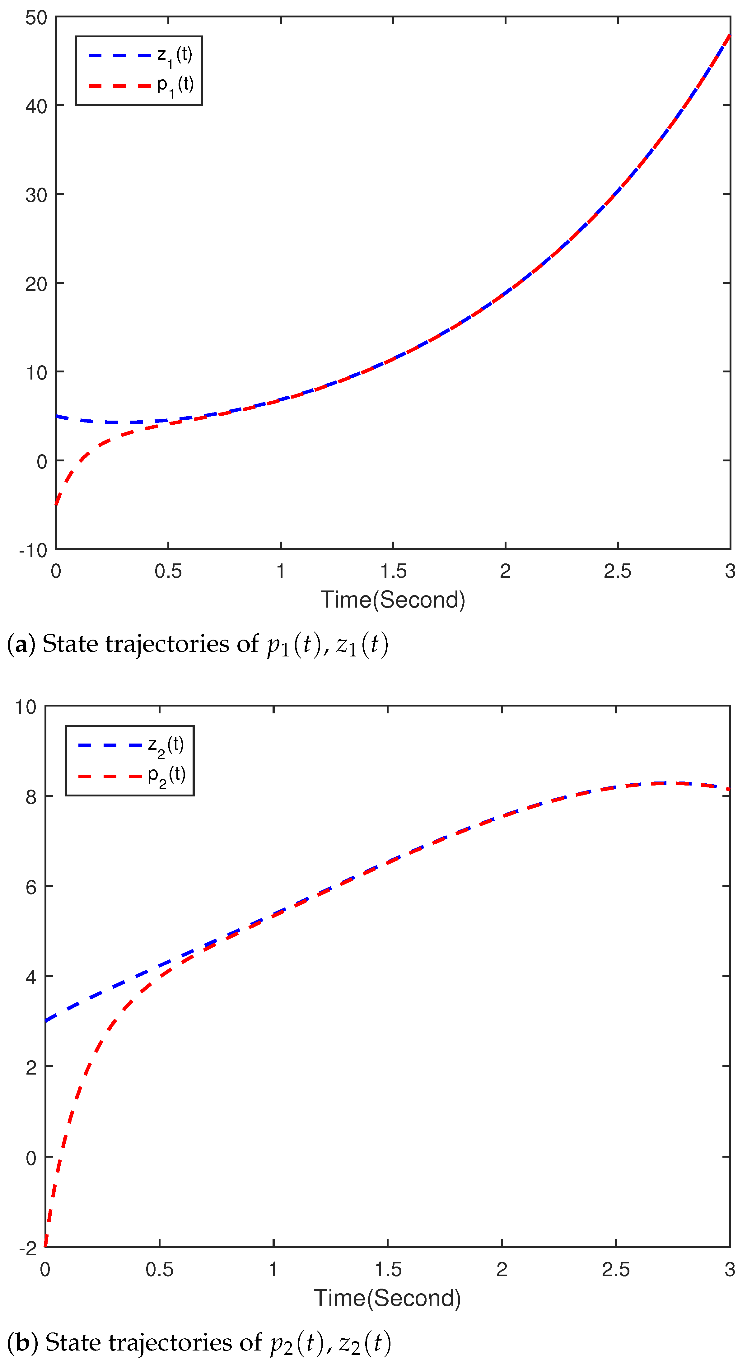
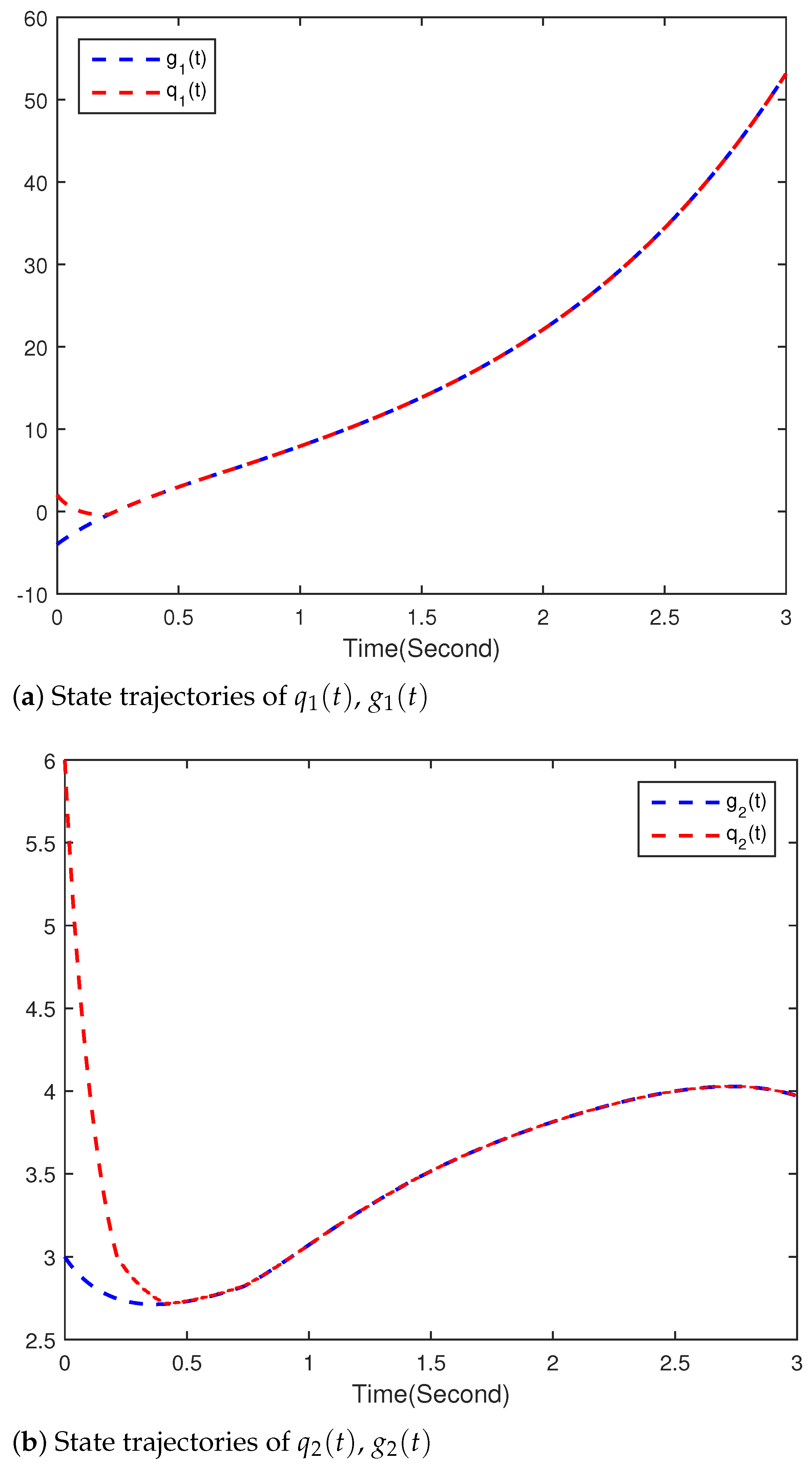
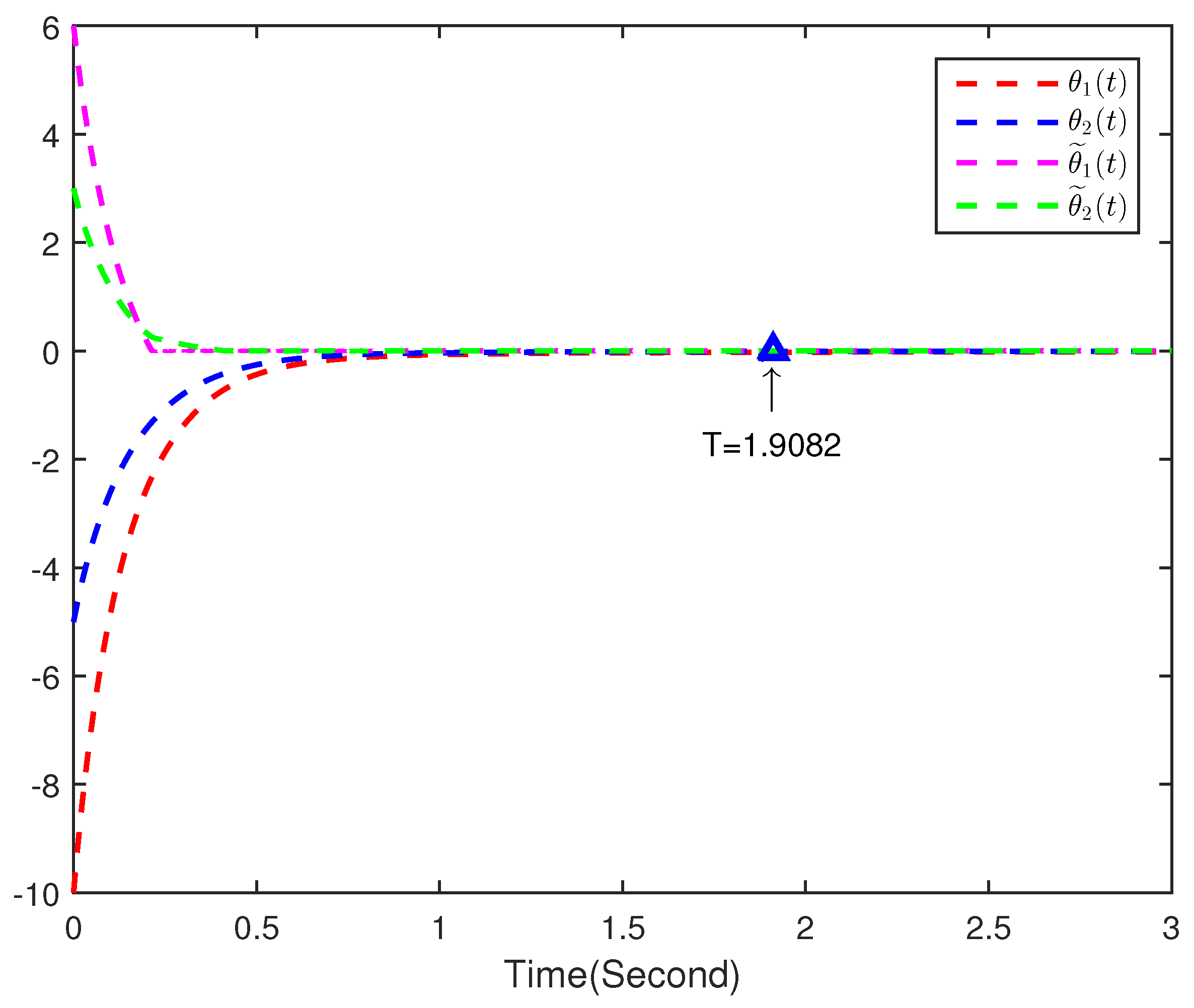
4. Numerical Simulations

In this section, we use two numerical examples to verify the validity of the results of Theorems 1 and 2.
Example 1.
Consider a two-dimensional FFINNs with piecewise activations and mixed delay.
The drive system is given by
D t α z k ( t ) = ξ k z i ( t ) + g k ( t ) D t α g k ( t ) = ϕ k g k ( t ) + δ k z k ( t ) + r = 1 2 c k r λ r ( t ) + r = 1 2 d k r t σ 0 ( t ) t λ r ( s ) d s + r = 1 2 g k r v r + r = 1 2 P k ν r + r = 1 2 α k r λ r ( t σ r ( t ) ) + r = 1 2 Q k ν r + r = 1 2 β k r λ r ( t σ r ( t ) ) + I k , k = 1 , 2
and the response system
D t α p k ( t ) = ξ k p k ( t ) + q k ( t ) + u k ( t ) D t α q k ( t ) = ϕ k q k ( t ) + δ k p k ( t ) + r = 1 2 c k r ζ r ( t ) + r = 1 2 d k r t σ 0 ( t ) t ζ r ( s ) d s + r = 1 2 g k r v r + r = 1 2 P k ν r + r = 1 2 α k r ζ r ( t σ r ( t ) ) + r = 1 2 Q k ν r + r = 1 2 β k r ζ r ( t σ r ( t ) ) + I k + u ˜ k ( t ) , k = 1 , 2 . ,
where
h k ( x ) = tanh ( x ) + 0.8 , x 0 tanh ( x ) 0.8 , x < 0 .
Obviously, h k ( x ) satisfies Assumptions 1 and 2 with L k = 1 , S k = 1 , k = 1 , 2 . The parameters of drive (33) and response (34) system are chosen as follows:
α = 0.95 ; a 1 = 3 , a 2 = 2 , b 1 = b 2 = 1 , ξ 1 = 0.2 , ξ 2 = 0.1 ; c 11 = c 21 = 0.1 , c 12 = 0.3 , c 22 = 0.2 α 11 = α 12 = α 21 = α 22 = 0.01 ; β 11 = β 12 = β 21 = β 22 = 0.1 ; d 11 = d 12 = d 21 = d 22 = 0.1 ; I 1 = 0.2 , I 2 = 0.5 , σ k ( t ) = 0.3 cos ( 2 t ) + 0.7 , k = 1 , 2 .
The controller is designed as follows:
u k ( t ) = k k e k ( t ) ρ s i g n e k ( t ) | e k ( t ) | μ + ω k | e k ( t σ k ( t ) ) | u ˜ k ( t ) = η k 1 e ˜ k ( t ) s i g n e ˜ k ( t ) η k 2 + ρ | e ˜ k ( t ) | μ r = 1 2 d k r t σ 0 ( t ) t ζ r ( s ) d s + r = 1 2 d k r t σ 0 ( t ) t λ r ( s ) d s . .
The controller parameters are as follows:
k 1 = 2 , k 2 = 2 , ω 1 = 1 , ω 2 = 1 , ρ = 4 ; η 11 = η 12 = η 21 = η 22 = 2 , μ = 0.8 .
The initial conditions are given as
z 1 ( t ) = 2 , z 2 ( t ) = 3 , g 1 ( t ) = 4 , g 2 ( t ) = 1 ; p 1 ( t ) = 4 , p 2 ( t ) = 1 , q 1 ( t ) = 2 , q 2 ( t ) = 4 .
The time T is calculated by Theorem 1, which means that (34) and (35) can achieve synchronization in a finite time T. Furthermore, here T = 1.7220 .
Figure 2, Figure 3 and Figure 4 show the simulation results of the drive(33) and response(34) system. Figure 2 and Figure 3 show the trajectories of states p ( t ) and z ( t ) , and q ( t ) and g ( t ) , respectively. Equation (34) indeed converges to (33) with the controller (35) in T, and the convergence error continues to remain zero. The time evolution of synchronization errors θ ( t ) and θ ˜ ( t ) between systems (33) and (34) are presented in Figure 4. Simulation results show that the main results of the finite-time synchronization entrenched are correct in this article.
Example 2.
Consider a two-dimensional FFINNs with piecewise activations and mixed delay.
The drive system is given by
D t α z k ( t ) = ξ k z k ( t ) + g k ( t ) D t α g k ( t ) = ϕ k g k ( t ) + δ k z k ( t ) + r = 1 2 c k r λ r ( t ) + r = 1 2 d k r t σ 0 ( t ) t λ r ( s ) d s + r = 1 2 g k r v r + r = 1 2 P k ν r + l = 1 2 α k r λ r ( t σ r ( t ) ) + r = 1 2 Q k ν r + r = 1 2 β k r λ r ( t σ r ( t ) ) + I k , k = 1 , 2 .
and the response system is given by
D t α p k ( t ) = ξ k p k ( t ) + q k ( t ) + u k ( t ) D t α q k ( t ) = ϕ k q k ( t ) + δ k p k ( t ) + r = 1 2 c k r ζ l ( t ) + r = 1 2 d k r t σ 0 ( t ) t ζ r ( s ) d s + r = 1 2 g k r v r + r = 1 2 P k ν r + r = 1 2 α k r ζ r ( t σ r ( t ) ) + r = 1 2 Q k ν r + r = 1 2 β k r ζ r ( t σ r ( t ) ) + I k + u ˜ k ( t ) , k = 1 , 2 ,
where
h k ( x ) = tanh ( x ) + 0.5 , x 0 tanh ( x ) 0.5 , x < 0 .
Obviously, h k ( x ) satisfies Assumptions 1 and 2 with L k = 1 , S k = 1 , k = 1 , 2 . The parameters of drive (33) and response (34) system are chosen as follows:
α = 0.95 ; a 1 = b 2 = 1 , a 2 = b 1 = 2 , ξ 1 = 0.2 , ξ 2 = 0.1 ; c 11 = c 21 = 0.2 , c 12 = c 22 = 0.1 α 11 = α 12 = α 21 = α 22 = 1 ; β 11 = β 12 = β 21 = β 22 = 0.5 ; d 11 = d 21 = 0.1 , d 12 = d 22 = 0.2 ; I 1 = 0.2 , I 2 = 0.5 , σ k ( t ) = 0.3 cos ( 2 t ) + 0.7 , k = 1 , 2 .
The controller is designed as follows:
u k ( t ) = k k 1 θ k ( t ) k k 2 s i g n θ k ( t ) | θ k ( t ) | μ u ˜ k ( t ) = η k 1 θ ˜ k ( t ) s i g n θ ˜ k ( t ) ( η k 2 | θ ˜ k ( t ) | μ + ω k | θ k ( t σ k ( t ) ) | + r = 1 2 L r | d k r | t σ 0 ( t ) t | θ r ( s ) | d s + ρ k ) .
The controller parameter is given by
k 11 = k 21 = 6 , k 12 = k 22 = 4 , ω 1 = 1.2 , ω 2 = 0.8 ; η 11 = η 21 = 6 , η 12 = η 21 = 2 , ρ 1 = ρ 2 = 9 , μ = 0.7 .
The initial conditions are given as
z 1 ( t ) = 5 , z 2 ( t ) = 3 , g 1 ( t ) = 4 , g 2 ( t ) = 3 ; p 1 ( t ) = 5 , p 2 ( t ) = 2 , q 1 ( t ) = 2 , q 2 ( t ) = 6 .
The time T is calculated by Theorem 2, which means that (37) and (38) can achieve synchronization in a finite time T. Furthermore, here T = 1.9082 .
Figure 5, Figure 6 and Figure 7 show the simulation results of the drive(36)-response(37) system. Figure 5 and Figure 6 show the trajectories of states p ( t ) and z ( t ) , q ( t ) and g ( t ) , respectively. Equation (37) indeed converges to (36) with the controller (38) in T, and the convergence error continues to remain zero. The time evolution of synchronization errors θ ( t ) and θ ˜ ( t ) between systems (36) and (37) are presented in Figure 7. Simulation results show that the main results of the finite-time synchronization entrenched are correct in this article.

5. Conclusions

In this paper, a class of fractional order fuzzy inertial cellular neural network system with piecewise activation and mixed delay is proposed, and the finite-time synchronization of the system is discussed. By using the finite-time stability theory, Lyapunov functionals, and analytical techniques, some novel methods for finite-time synchronization of drive-response systems are obtained. Finally, two numerical simulation examples show that the proposed method is effective. In the future, we propose to expand our results to better apply FFINNs and implement it by designing hardware. The more efficient control laws will be considered, which is a challenging topic.

Author Contributions

Conceptualization, methodology, writing—original draft preparation, Y.L. and Y.S.; writing—review and editing, numerical simulation, Y.L.; project administration, Y.S. All authors have read and agreed to the published version of the manuscript.

Funding

This work was partly supported by the Natural Science Foundation of Anhui Province (2008085MF200), the Program for Innovative Research Team in Universities of Anhui Province (2022AH010085), the University Natural Science Foundation of Anhui Province (KJ2021A0970), the National Natural Science Foundation of China (61403157), the Research and Development Plan Project Foundation of Huainan (2021A248).

Data Availability Statement

The data presented in this study are available in the article.

Acknowledgments

The authors would like to thank the anonymous referees and reviewers for their helpful comments, which have significantly improved the quality of the presentation.

Conflicts of Interest

The authors declare no conflict of interest.

References

  1. Yang, T.; Yang, L. The global stability of fuzzy cellular neural network. IEEE Trans. Circuits Syst. I 1996, 43, 880–883. [Google Scholar] [CrossRef]
  2. Yang, T.; Yang, L.; Wu, C.W.; Chua, L.O. Fuzzy cellular neural networks: Applications. In Proceedings of the 1996 Fourth IEEE International Workshop on Cellular Neural Networks and Their Applications Proceedings (CNNA-96), Seville, Spain, 24–26 June 1996; pp. 225–230. [Google Scholar]
  3. Yang, T.; Yang, L. Fuzzy cellular neural network: A new paradigm for image processing. Int. J. Circ. Theory Appl. 1997, 25, 469–481. [Google Scholar] [CrossRef]
  4. Shitong, W.; Min, W. A new detection algorithm (NDA) based on fuzzy cellular neural networks for white blood cell detection. IEEE Trans. Inf. Technol. Biomed. 2006, 10, 5–10. [Google Scholar] [CrossRef]
  5. Wang, S.; Fu, D.; Xu, M.; Hu, D. Advanced fuzzy cellular neural network: Application to CT liver images. Artif. Intell. Med. 2007, 39, 65–77. [Google Scholar] [CrossRef]
  6. Balasubramaniam, P.; Kalpana, M.; Rakkiyappan, R. Stationary oscillation of interval fuzzy cellular neural networks with mixed delays under impulsive perturbations. Neural Comput. Appl. 2013, 22, 1645–1654. [Google Scholar] [CrossRef]
  7. Ratnavelu, K.; Manikandan, M.; Balasubramaniam, P. Design of state estimator for BAM fuzzy cellular neural networks with leakage and unbounded distributed delays. Inf. Sci. 2017, 397, 91–109. [Google Scholar] [CrossRef]
  8. Hurtik, P.; Molek, V.; Hula, J. Data preprocessing technique for neural networks based on image represented by a fuzzy function. IEEE Trans. Fuzzy Syst. 2020, 28, 1195–1204. [Google Scholar] [CrossRef]
  9. Guan, C.; Wang, S.; Liew, A.W. Lip image segmentation based on a fuzzy convolutional neural network. IEEE Trans. Fuzzy Syst. 2020, 28, 1242–1251. [Google Scholar] [CrossRef]
  10. Chen, L.; Su, W.; Wu, M.; Pedrycz, W.; Hirota, K. A fuzzy deep neural network with sparse autoencoder for emotional intention understanding in human-robot interaction. IEEE Trans. Fuzzy Syst. 2020, 28, 1252–1264. [Google Scholar] [CrossRef]
  11. Babcock, K.; Westervelt, R. Stability and dynamics of simple electronic neural networks with added inertia. Phys. D Nonlinear Phenom. 1986, 23, 464–469. [Google Scholar] [CrossRef]
  12. Wan, P.; Jian, J. Global convergence analysis of impulsive inertial neural networks with time-varying delays. Neurocomputing 2017, 245, 68–76. [Google Scholar] [CrossRef]
  13. Zhang, G.; Zeng, Z.; Hu, J. New results on global exponential dissipativity analysis of memristive inertial neural networks with distributed time-varying delays. Neural Netw. 2018, 97, 183–191. [Google Scholar] [CrossRef] [PubMed]
  14. Aouiti, C.; Gharbia, I.B.; Cao, J.; Alsaedi, A. Dynamics of impulsive neutral-type BAM neural networks. J. Frankl. Inst. 2019, 356, 2294–2324. [Google Scholar] [CrossRef]
  15. Aouiti, C.; Assali, E.A. Nonlinear Lipschitz measure and adaptive control for stability and synchronization in delayed inertial Cohen-Grossberg-type neural networks. Int. J. Adapt. Control Signal Process. 2019, 33, 1457–1477. [Google Scholar] [CrossRef]
  16. Chaouki, A.; El Abed, A. Finite-time and fixed-time synchronization of inertial neural networks with mixed delays. J. Syst. Sci. Complex. 2021, 34, 206–235. [Google Scholar] [CrossRef]
  17. Lu, J.; Chen, Y. Robust stability and stabilization of fractional-order interval systems with the fractional order α: The 0 < α < 1 case. IEEE Trans. Autom. Control 2010, 55, 152–158. [Google Scholar]
  18. Liao, C.; Lu, C. Design of delay-dependent state estimator for discrete-time recurrent neural networks with interval discrete and infinite-distributed timevarying delays. Cognit. Neurodyn. 2011, 5, 133–143. [Google Scholar] [CrossRef] [Green Version]
  19. Li, L.; Sun, Y. Adaptive Fuzzy Control for Nonlinear Fractional-Order Uncertain Systems with Unknown Uncertainties and External Disturbance. Entropy 2015, 17, 5580–5592. [Google Scholar] [CrossRef] [Green Version]
  20. Zhang, S.; Chen, Y.; Yu, Y. A survey of fractional-order neural networks. In Proceedings of the ASME 2017 International Design Engineering Technical Conferences and Computers and Information in Engineering Conference, Cleveland, OH, USA, 6–9 August 2017. [Google Scholar]
  21. Ma, Z.; Ma, H. Adaptive fuzzy backstepping dynamic surface control of strict-feedback fractional-order uncertain nonlinear systems. IEEE Trans. Fuzzy Syst. 2020, 28, 122–133. [Google Scholar] [CrossRef]
  22. Zhang, Q.; Lu, J. Bounded real lemmas for singular fractional-order systems: The 1 < α < 2 case. IEEE Trans. Circuits Syst. II Express Briefs 2021, 68, 732–736. [Google Scholar]
  23. Yang, Z.; Zhang, Z. Global asymptotic synchronisation of fuzzy inertial neural networks with time-varying delays by applying maximum-value approach. Int. J. Syst. Sci. 2022, 53, 2281–2300. [Google Scholar] [CrossRef]
  24. Feng, Y.; Xiong, X.; Tang, R.; Yang, X. Exponential synchronization of inertial neural networks with mixed delays via quantized pinning control. Neurocomputing 2018, 310, 165–171. [Google Scholar] [CrossRef]
  25. Zhang, S.; Tang, M.; Liu, X. Synchronization of a Riemann–Liouville fractional time-delayed neural network with two inertial terms. Circuits Syst. Signal Process. 2021, 40, 5280–5308. [Google Scholar] [CrossRef]
  26. Tang, Q.; Jian, J. Exponential synchronization of inertial neural networks with mixed time-varying delays via periodically intermittent control. Neurocomputing 2019, 338, 181–190. [Google Scholar] [CrossRef]
  27. Liang, K.; Li, W. Exponential synchronization in inertial Cohen–Grossberg neural networks with time delays. J. Frankl. Inst. 2019, 356, 11285–11304. [Google Scholar] [CrossRef]
  28. Shi, J.; Zeng, Z. Global exponential stabilization and lag synchronization control of inertial neural networks with time delays. Neural Netw. 2020, 126, 11–20. [Google Scholar] [CrossRef]
  29. Zhang, Z.; Cao, J. Finite-time synchronization for fuzzy inertial neural networks by maximum value approach. IEEE Trans. Fuzzy Syst. 2021, 30, 1436–1446. [Google Scholar] [CrossRef]
  30. Hua, L.; Zhong, S.; Shi, K.; Zhang, X. Further results on finite-time synchronization of delayed inertial memristive neural networks via a novel analysis method. Neural Netw. 2020, 127, 47–57. [Google Scholar] [CrossRef]
  31. Chen, C.; Li, L.; Peng, H.; Yang, Y. Fixed-time synchronization of inertial memristor-based neural networks with discrete delay. Neural Netw. 2019, 109, 81–89. [Google Scholar] [CrossRef] [PubMed]
  32. Alimi, A.; Aouiti, C.; Assali, E.A. Finite-time and fixed-time synchronization of a class of inertial neural networks with multi-proportional delays and its application to secure communication. Neurocomputing 2019, 332, 29–43. [Google Scholar] [CrossRef]
  33. Yang, T.; Zou, R.; Liu, F. Finite/fixed-time synchronization control of fuzzy inertial cellular neural networks with mixed delays. Trans. Inst. Meas. Control 2023. [Google Scholar] [CrossRef]
  34. Podlubny, I. Fractional Differential Equations; Academic Press: New York, NY, USA, 1999. [Google Scholar]
  35. Li, C.; Deng, W. Remarks on fractional derivatives. Appl. Math. Comput. 2007, 187, 777–784. [Google Scholar] [CrossRef]
  36. Lakshmikantha, V.; Leela, S.; Devi, J. Theory of Fractional Dynamic Systems; Cambridge Scientific Publishers: Cambridge, UK, 2009. [Google Scholar]
  37. Zhang, S.; Yu, Y.; Wang, H. Mittag-Leffler stability of fractional-order Hopfield neural networks. Nonlinear Anal. Hybrid Syst. 2015, 16, 104–121. [Google Scholar] [CrossRef]
  38. Aguila, C.; Duarte-Mermoud, M.; Gallegos, J. Lyapunov functions for fractional order systems. Commun. Nonlinear Sci. Simul. 2014, 19, 2951–2957. [Google Scholar] [CrossRef]
  39. Kong, F.; Zhu, Q.; Sakthivel, R. Finite-time and fixed-time synchronization analysis of fuzzy Cohen-Grossberg neural networks with piecewise activations and parameter uncertainties. Eur. J. Control 2020, 56, 179–190. [Google Scholar] [CrossRef]
  40. Li, H.; Cao, J.; Jiang, H.; Alsaedi, A. Graph theory-based finite-time synchronization of fractional-order complex dynamical networks. J. Frankl. Inst. 2018, 355, 5771–5789. [Google Scholar] [CrossRef]
  41. Duan, L.; Jian, J.; Wang, B. Global exponential dissipativity of neutral-type BAM inertial neural networks with mixed time-varying delays. Neurocomputing 2020, 378, 399–412. [Google Scholar] [CrossRef]
  42. Syed Ali, M.; Narayanan, G.; Shekher, V.; Alsaedi, A.; Ahmad, B. Global Mittag-Leffler stability analysis of impulsive fractional-order complex-valued BAM neural networks with time varying delays. Commun. Nonlinear Sci. Numer. Simul. 2020, 83, 105088. [Google Scholar] [CrossRef]
  43. Chen, L.; Huang, T.; Machado, J.A.T.; Lopes, A.M.; Chai, Y.; Wu, R. Delay-dependent criterion for asymptotic stability of a class of fractional-order memristive neural networks with time-varying delays. Neural Netw. 2019, 118, 289–299. [Google Scholar] [CrossRef]
Figure 1. Framework of feedback control.
Fractalfract 07 00294 g001
Figure 2. Time responses of p ( t ) and z ( t ) .
Fractalfract 07 00294 g002
Figure 3. Time responses of q ( t ) and g ( t ) .
Fractalfract 07 00294 g003
Figure 4. Synchronization error θ ( t ) and θ ˜ ( t ) between the drive-response system
Fractalfract 07 00294 g004
Figure 5. Time responses of p ( t ) and z ( t ) .
Fractalfract 07 00294 g005
Figure 6. Time responses of q ( t ) and g ( t ) .
Fractalfract 07 00294 g006
Figure 7. Synchronization error θ ( t ) and θ ˜ ( t ) between the drive-response system.
Fractalfract 07 00294 g007
Disclaimer/Publisher’s Note: The statements, opinions and data contained in all publications are solely those of the individual author(s) and contributor(s) and not of MDPI and/or the editor(s). MDPI and/or the editor(s) disclaim responsibility for any injury to people or property resulting from any ideas, methods, instructions or products referred to in the content.

